Numerical Investigation of the Flow Field and Mass Transfer Characteristics in a Jet Slurry Pump

Abstract

A jet pump is used to transport a variety of working media and is especially suitable for dredged soil transporting. In this study, a three-dimensional numerical study of a jet pump that is used for slurry delivery was carried out. The characteristics of the internal flow field of the mixing chamber with different working parameters were comprehensively analyzed. The results indicate that the pressure of the axial line decreases with increasing flow ratio (ratio of suction flux and inlet flux) while the pressure of the injected slurry shows a downward trend. With the increase in the flow ratio, the pressure ratio (difference between inlet pressure and suction pressure divided by the difference between exit pressure and suction pressure) falls off while the efficiency presents a parabolic distribution. The pressure ratio can be promoted by properly increasing the length of the mixing chamber so that the available efficiency is broadened. When the mixing chamber length is L = 2.5D_n~4.0D_n (D_n is nozzle outlet diameter), the highly efficient area is wide; in particular, when L = 3.5D_n, the jet slurry pump with the highest efficiency of 27.6% has the best performance.

1. Introduction

In dredging projects, slurry and sand are the main operating objects. Slurry transport systems are complicated and a key component in dredging systems [1]. The concentration distribution, deposition rate and mixing effect of the slurry, a mixture of sand and water, are strictly controlled in transportation processes, which are closely related to dredging efficiency and dredging benefits [2,3].

Due to its simple structure, a jet pump is used to transport the majority of working media, and it is especially suitable for dredged soil transport [4,5,6]. Its working principle is transferring mass and heat through turbulent diffusion between the primary and secondary flows [7]. The advantages of reliable operation, low cost and easy maintenance [8] make it widely used in many industrial fields, such as the refrigeration industry [9], water conservancy engineering [10], aerospace engineering [11], chemical industry [12] and fish farming [13]. Previous studies have shown that the performance of the jet pump is greatly affected by the construction dimensions [14,15,16] and operating conditions [17,18,19]. Furthermore, the two-phase flow in a jet pump is a complex turbulent flow with an irregular flowing discipline [20]. Therefore, it is necessary to deeply illuminate the flow state in the jet slurry pump for more efficient utilization.

In terms of the internal flow field, a series of studies on jet pumps have been conducted, and outstanding results have been obtained by researchers from various countries. Mallela R. et al. [21] conducted a numerical study and found that the energy loss of a jet pump was mainly caused by improper mixing of the primary and secondary streams, which formed recirculation near the throat inlet. Based on this, the standardized length of the mixing tube was proposed to be 7 to 9 times the diameter. Girgidov A.D. [22] conducted an experimental study on a jet pump used for liquid transportation according to the hydraulic configuration, and pointed out the optimization interval of the independent variables to guide the design of jet pumps. Banasiak K. et al. [23] proved that the efficiency of the jet pump greatly depends on the length and diameter of the throat and the divergence angle of the diffuser. Compared with the conventional expansion valve system, the maximum increase in the coefficient of performance was 8%. Long X.P. et al. [24] conducted a numerical study on the thickness of the nozzle outlet tip in the structure of the jet pump and found that the distribution of turbulent kinetic energy was affected. The results revealed that the vortex was promoted when the nozzle outlet tip thickened or the flow ratio increased. The performance of the jet pump was optimal when the thickness was 0.2~0.6 mm. Yang X.L. and Long X.P. [25] studied the effects of different turbulence models and wall boundary treatment methods on jet pump performance and the internal flow field. The results showed that when the flow ratio became quite high, the numerical errors of various combinations were greater than 10%, but the errors of some combinations could be reduced by modifying the turbulence model constants. The area ratio of the 0.25 jet pump was investigated by Kumar R.S. et al. [26]. The performance of the jet pump was analyzed by generating equal efficiency curves on various primary flows, which found the optimal mixing chamber length for the jet pump and the corresponding maximum efficiency.

In terms of numerical computation, many relevant works have been done. Yasmin H. and Iqbal N. [27,28,29,30] performed a series of fruitful studies on the numerical simulation of peristaltic fluid flow. Du W. et al. [31] numerically investigated the interaction effects of the latticework duct and jet cooling structures on the flow structure and heat transfer. Results showed that the flow field and heat transfer characteristics were sensitive to the jet nozzle location, shapes and mass flow ratios. Zhou L. et al. [32] studied a high-speed electrical submersible pump with different end clearances, which showed that an increase in the end clearance led to a decrease in the head and efficiency of the electrical submersible pump.

The above research results demonstrate some progresses, but the research has mainly focused on water suction, while there is little research on slurry delivery by jet pump. A jet pump has its unique advantages in some contexts because there are no rotating parts. Some already use jet pumps to pump mud in dredging projects. Based on this, we calculated the internal flow details and operating performance curve of a jet slurry pump of a certain size by drawing from previous research ideas on jet pumps.

In this paper, the jet pump used for slurry was numerically investigated based on the k-ε turbulence model and Mixture two-phase flow model. By changing the structure parameters and working conditions, the flow details in the jet pump were comprehensively analyzed and discussed. Finally, the operation curve and efficiency curve within the scope of this paper were obtained. The research results can be used as the theoretical basis for the selection and design of jet slurry pumps in dredging engineering.

2. Numerical Method

2.1. Jet Pump Parameters

Because there are no moving parts (impellers, etc.), the efficiency of jet slurry pumps is usually not high [33,34]. However, they have unique applications in some particular circumstances. Except for the working environments being different, there are some operating characteristics of jet slurry pumps that are the same as ordinary single-phase jet pumps, and the efficiency still depends on a few main parameters in jet pump theory, such as the nozzle structure [8], area ratio [35] and flow ratio [36]. These parameters [37] of the area ratio m, flow ratio M, pressure ratio H and efficiency η of the jet pump are defined as follows:

$$\mathrm{m}=\frac{S_{\mathrm{t}}}{S_n}$$

(1)

$$M=\frac{Q_s}{Q_o}$$

(2)

$$\mathrm{H}=\frac{{\mathrm{P}}_e-P_s}{P_o-P_s}$$

(3)

$$\eta =\frac{\mathrm{MH}}{1-H}$$

(4)

where the subscript s is the suction chamber, o is the nozzle inlet, n is the nozzle outlet, t is the throat, and e is the pump exit.

2.2. Governing Equations and Turbulence Models

Because the hydraulic transport contains the relative velocity between the two phases, the two-phase jet pump is simulated by using the Mixture method [38] to establish the governing equation of the liquid–solid two-phase inside the jet slurry pump to study the incompressibility of the two phases. The fluid mixing process mainly solves the continuity equation, the momentum equation and the energy equation [39].

The continuity equation for the mixture is

$$\frac{\partial }{\partial t}\left({\rho }_m\right)+\nabla ·\left({\rho }_m{\overrightarrow{v}}_m\right)=0$$

(5)

where ${\overrightarrow{v}}_m$ is the mass-averaged velocity and ${\rho }_m$ is the mixture density.

The momentum equation for the mixture can be expressed as

$$\frac{\partial }{\partial t}\left({\rho }_m{\overrightarrow{v}}_m\right)+\nabla ·\left({\rho }_m{\overrightarrow{v}}_m{\overrightarrow{v}}_m\right)=-\nabla p+\nabla ·\left[{\mu }_m\left(\nabla {\overrightarrow{v}}_m+\nabla {\overrightarrow{v}}_m^T\right)\right]+{\rho }_m\overrightarrow{g}+\overrightarrow{F}+\nabla ·\left({\displaystyle \sum _{k=1}^n{\alpha }_k}{\rho }_k{\overrightarrow{v}}_{dr,k}{\overrightarrow{v}}_{dr,k}\right)$$

(6)

where n is the number of phases, $\overrightarrow{F}$ is the body force, ${\mu }_m$ is the viscosity of the mixture, and ${\overrightarrow{v}}_{dr,k}$ is the drift velocity for secondary phase k.

The energy equation for the mixture takes the following form:

$$\frac{\partial }{\partial t}{\displaystyle \sum _{k=1}^n\left({\alpha }_k{\rho }_k{E}_k\right)}+\nabla ·{\displaystyle \sum _{k=1}^n\left({\alpha }_k{\overrightarrow{v}}_k\left({\rho }_k{E}_k+p\right)\right)}=\nabla ·\left(k_{eff}\nabla T\right)+S_E$$

(7)

where $k_{eff}$ is the effective conductivity (${\displaystyle \sum _{}^{}{\alpha }_{\mathrm{k}}{(\mathrm{k}}_{\mathrm{k}}{+\mathrm{k}}_{\mathrm{t}})}$), where ${\mathrm{k}}_{\mathrm{t}}$ is the turbulent thermal conductivity, defined according to the turbulence model being used. $S_E$ includes any other volumetric heat sources. ${\mathrm{E}}_{\mathrm{k}}=h_k-\frac{p}{p_k}+\frac{v_k^2}{2}$ for a compressible phase, and ${\mathrm{E}}_{\mathrm{k}}=h_k$ for an incompressible phase, where $h_k$ is the sensible enthalpy for phase k.

The standard k-ε model is selected. The turbulence kinetic energy, k, and its rate of dissipation, ε, are obtained from the following transport equations:

$$\frac{\partial }{\partial t}(\rho k)+\frac{\partial }{\partial x_i}\left(\rho k{u}_i\right)=\frac{\partial }{\partial x_j}\left[\left(\mu +\frac{{\mu }_t}{{\sigma }_k}\right)\frac{\partial k}{\partial x_j}\right]+G_k+G_b-\rho \epsilon -Y_M+S_k$$

(8)

and

$$\frac{\partial }{\partial t}(\rho \epsilon )+\frac{\partial }{\partial x_i}\left(\rho \epsilon u_i\right)=\frac{\partial }{\partial x_j}\left[\left(\mu +\frac{{\mu }_t}{{\sigma }_{\epsilon }}\right)\frac{\partial \epsilon }{\partial x_j}\right]+C_{1\epsilon }\frac{\epsilon }{k}\left(G_k+C_{3\epsilon }{G}_b\right)-C_{2\epsilon }\rho \frac{{\epsilon }^2}{k}+S_{\epsilon }$$

(9)

In these equations, G_K represents the generation of turbulence kinetic energy due to the mean velocity gradients. G_b is the generation of turbulence kinetic energy due to buoyancy. Y_M represents the contribution of the fluctuating dilatation incompressible turbulence to the overall dissipation rate. C_1ε, C_2ε and C_3ε are constants. σ_k and σ_e are the turbulent Prandtl numbers for k and ε, respectively. S_k and S_ε are user-defined source terms.

2.3. Modeling and Meshing

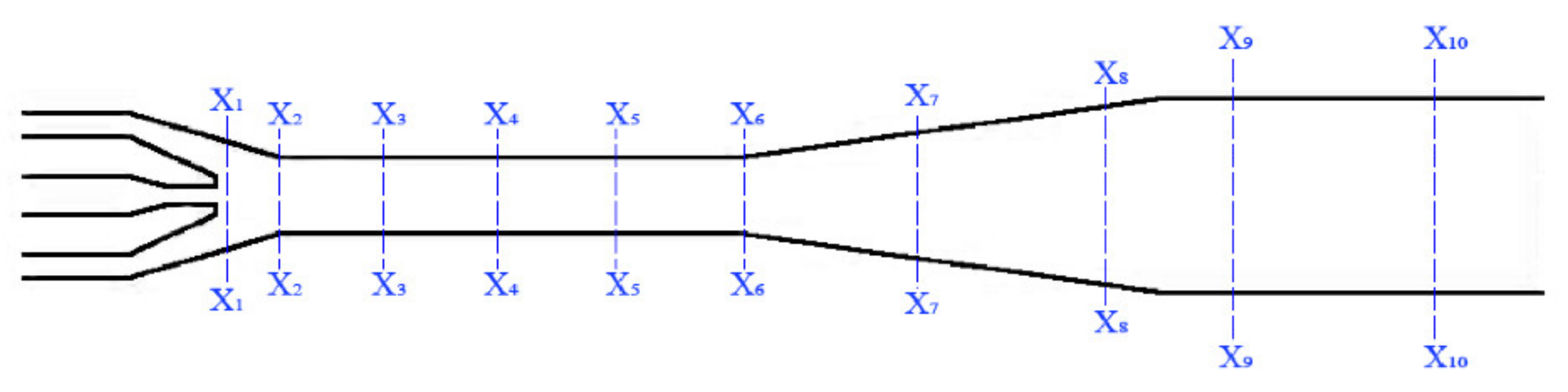
2.3.1. 3D Geometrical Model

Based on the requirements of the two-phase jet pump and the references [40,41], the cone straight nozzle was used, while the suction tube was simplified. The schematic diagram and main parameters of the jet pump is shown in Figure 1. The three-dimensional model of the calculation domain was completed as shown in Figure 2, and the main geometrical parameters are shown in

Table 1. Geometric parameters of the jet slurry pump.

Nozzle Inlet Di (mm)	Nozzle Inlet Angle α (°)	Nozzle Outlet Diameter Dn (mm)	Mixing Chamber Length L (mm)	Throat Diameter Dt (mm)	Mixing Tube Length Lt (mm)	Angle of Diffuser Inlet β (°)	Diffuser Length Ld (mm)	Area Ratio m
16	13.8	8	8	32	192	8	180	16

.

2.3.2. Gridding

To reduce the calculation cost and ensure calculation accuracy in the simulation, a structured grid was generated. In addition, the geometrical model appropriately extends the length of the jet pump outlet. In particular, the grid density of the area with a large pressure and velocity gradient (nozzle outlet and mixing chamber and throat upstream) was increased for local adaption [42] (shown in Figure 3).

2.3.3. Grid Independence Test

In this study, the outlet pressure Pe of the model was selected as a reference value, and the model was meshed with different quantities of grid elements. Then, the same boundary conditions were used for the simulated calculation. The data results can be seen in

Table 2. Changes in the outlet pressure in different elements of the grid.

Elements of the Grid	Outlet Pressure Pe (Pa)	Deviation
637,845	−119,145	32.32%
883,452	−149,350	15.16%
1,030,459	−164,324	6.66%
1,327,280	−176,020	0.014%
1,548,932	−176,002	0.024%
1,762,390	−176,045	--

. It is evident that when the number of elements in the grid increases to 1,327,280, the Pe no longer decreases obviously, and the flow field simulation solution is basically stable and reliable. In line with the principle of accuracy and cost-saving calculation, approximately 1.32 million grids were selected for all the cases.

2.4. Boundary Conditions

The working fluid medium was liquid water, and the injected fluid slurry was defined as a 20% volume fraction of a sand water mixture, while the density of sand was 2.65 kg/m³. The Mixture model was adopted to solve the two-phase flow. The boundary conditions of the working fluid were the velocity inlet, the secondary flow slurry was the velocity inlet and the pump exit was the outflow. The independent variable M was adjusted by changing the two-phase flow rate. The PISO algorithm was used to solve the coupling of the velocity and pressure, and the second-order upwind scheme was used to reduce the effect of false dissipation. The time step was 5×10⁻⁴ s. The residual error of each calculation condition was less than 10⁻⁴, and the relative error was less than 0.5% as the convergence standard.

3. Results and Discussion

3.1. Validation

Yu G.L. et al. [43] conducted experimental research on a liquid and liquid–gas jet pump and the performance curves were obtained through characteristic experiments. The numerical investigation results were compared with the experimental data in the literature [43] to verify the reliability of the simulation results in this paper. The jet pump with an area ratio of m = 1.92 was selected to simulate the working condition with a gas content of 0 (liquid–liquid), and the relationship between the dimensionless parameter H-M is shown in Figure 4. As shown in the figure, the simulated value is in good agreement with the experimental value, and the range of error is −7.7%~1.5%. It is proven that the numerical simulation can be considered reliable.

3.2. Flow Field Analysis at the Axis of the Jet Slurry Pump

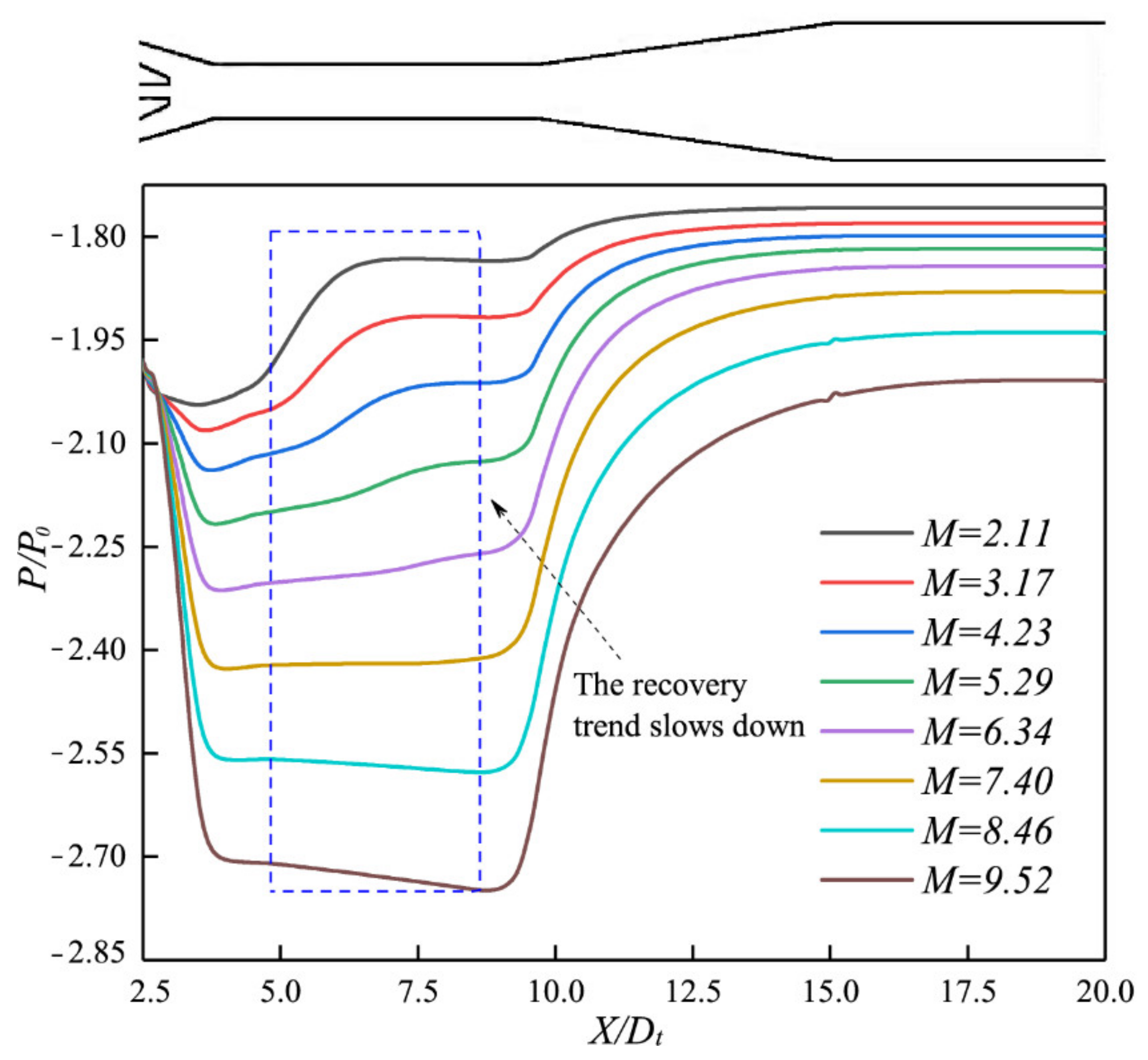
3.2.1. Pressure Distribution

Figure 5 shows the axial pressure distribution from nozzle inlet to exit. The pressure continued to decrease after the fluid entered the mixing chamber. This is because the high-speed working fluid and low-speed slurry exhibited a certain angle of convergence, which caused a large amount of energy loss. The lowest pressure was at X/D_t = 4~9 in the mixing tube. The pressure then increased slowly due to the gradual mixing of the two-phase flow. It is worth noting that the pressure increased faster at a low flow rate and mainly occurred downstream of the mixing tube. When M = 7.40, the minimum negative pressure was P_min = 2.5 × 10⁻⁵ Pa, the negative pressure in the suction chamber was strengthened, and the suction performance of the slurry was optimized. When M ≥ 8.46, the pressure from the throat to the diffuser continued to decrease. The lowest pressure appeared at the tail of the mixing tube. This is because when the flow ratio was too high, the slurry flow rate increased faster, thus losing more kinetic energy during the mixing process, resulting in a continuous pressure decrease [44] and the growing distance of the mixing process.

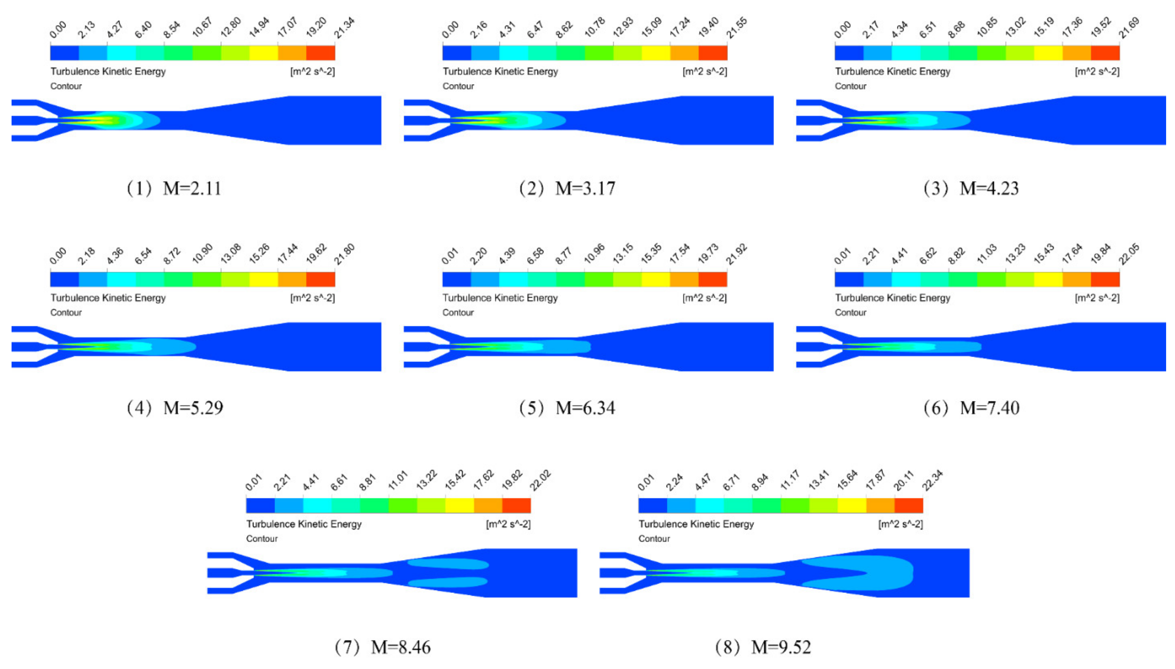
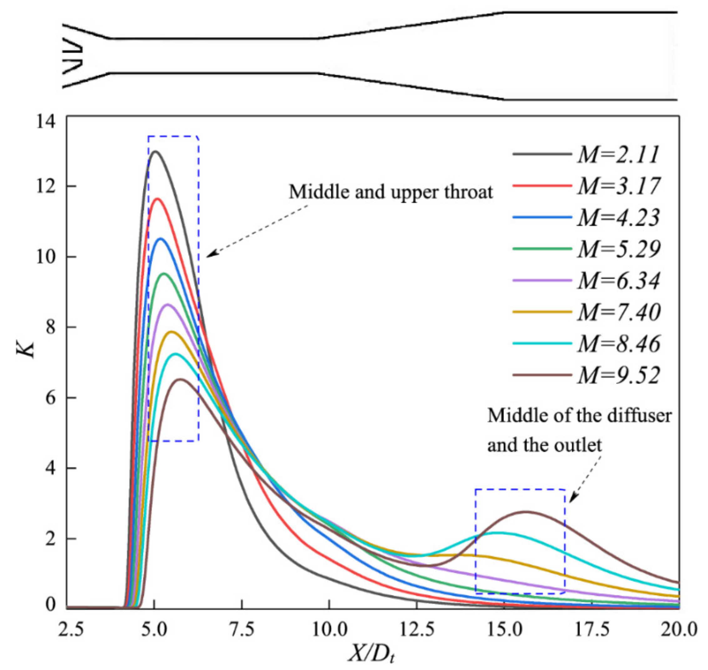
3.2.2. Turbulent Kinetic Energy Distribution

The distribution of turbulent kinetic energy along the axis direction at different flow ratios is shown in Figure 6. Under the low flow ratios of M = 2.11 and 3.17, the turbulent kinetic energy was mainly distributed in the middle of the mixing tube and near the pipe wall. As the flow ratio increased, the turbulent kinetic energy distribution began to narrow and elongate once it expanded downstream. When the flow ratio further increased, it appeared along the diffuser, and the flow field near the wall became unstable. This is because the difference in the velocity of the two fluids became more significant, and it was not completely mixed when reaching the diffuser.

The distribution of the axial turbulent kinetic energy is presented in Figure 7. The turbulent kinetic energy in the mixing chamber was 0. Intense momentum exchange happened in the middle of the mixing tube, with the turbulent kinetic energy rising sharply. Then, the turbulent kinetic energy started to decrease until it gradually stabilized in the diffuser. As the flow ratio increased, the peak value of the turbulent kinetic energy curve dropped. After reaching the peak, the turbulent kinetic energy decreased rapidly at a low flow ratio. At a high flow ratio, the turbulent kinetic energy decreased more gently compared to that at a low flow ratio. When the flow ratio was M ≥ 7.40, a secondary peak appeared in the diffuser, and the turbulent kinetic energy was consistent with the results in Figure 7. This is because the sudden change at the large cross-area of the mixed fluid entering the diffuser will cause a higher turbulent kinetic energy [45], which will interfere with the normal operation of the jet slurry pump.

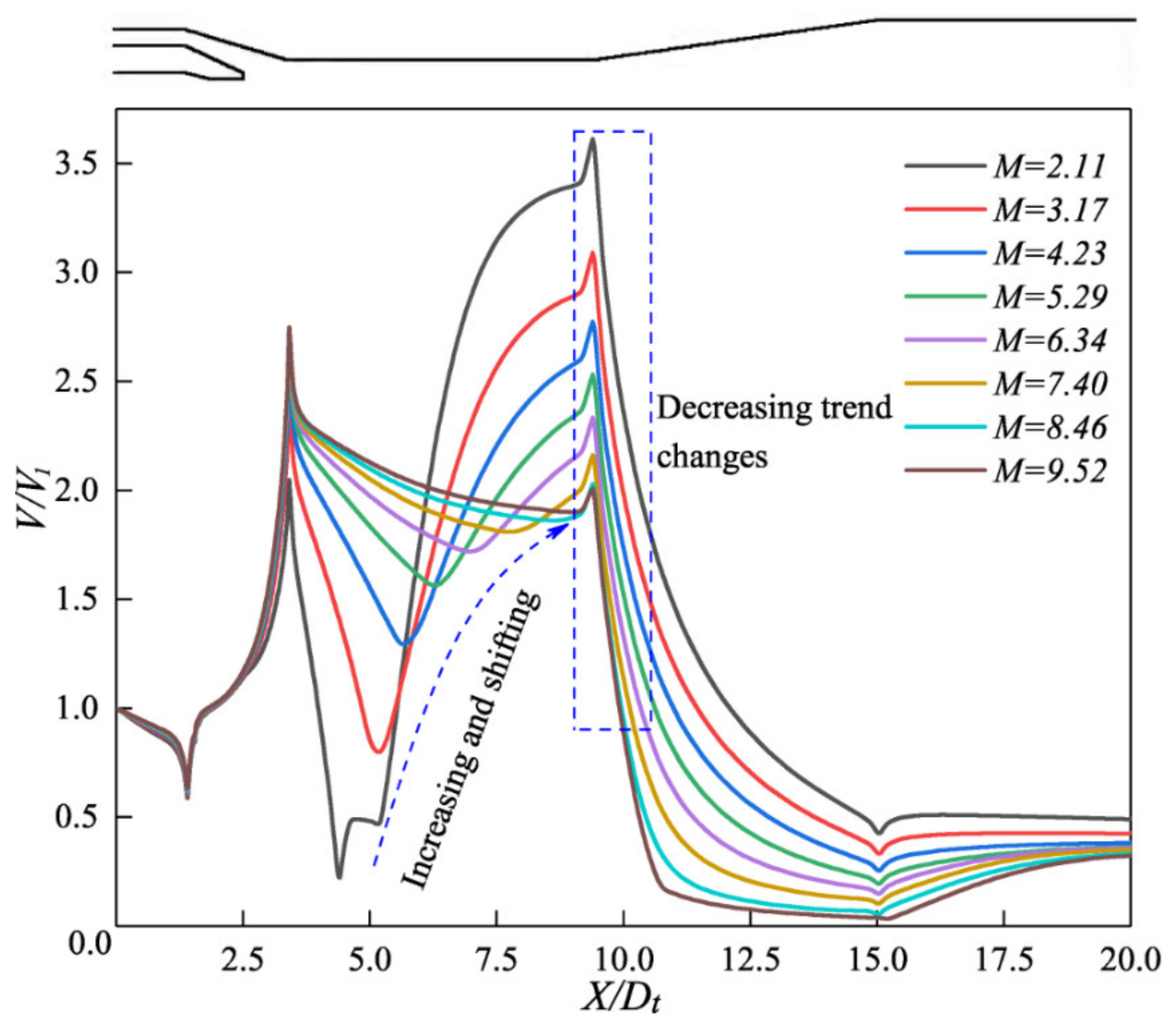
3.2.3. Velocity Distribution

In Figure 8, the velocity distribution of the shaft axis from nozzle inlet to exit is presented. When the high-speed fluid was at the front of the mixing chamber, the velocity core remained unchanged, but it began to decrease significantly after the mixing process through the mixing tube. The mixed energy of the two fluids became larger as the secondary flow rate increased, and the primary flow continued to accelerate in the mixing chamber. For low flow ratios, such as M = 2.11 and 3.17, the velocity at the mixing tube outlet was unchanged. This means that the mixing tube had a small effect on reducing the flow rate, which led to more flow losses by increasing the length of the mixing tube in this case.

3.3. Slurry Flow State

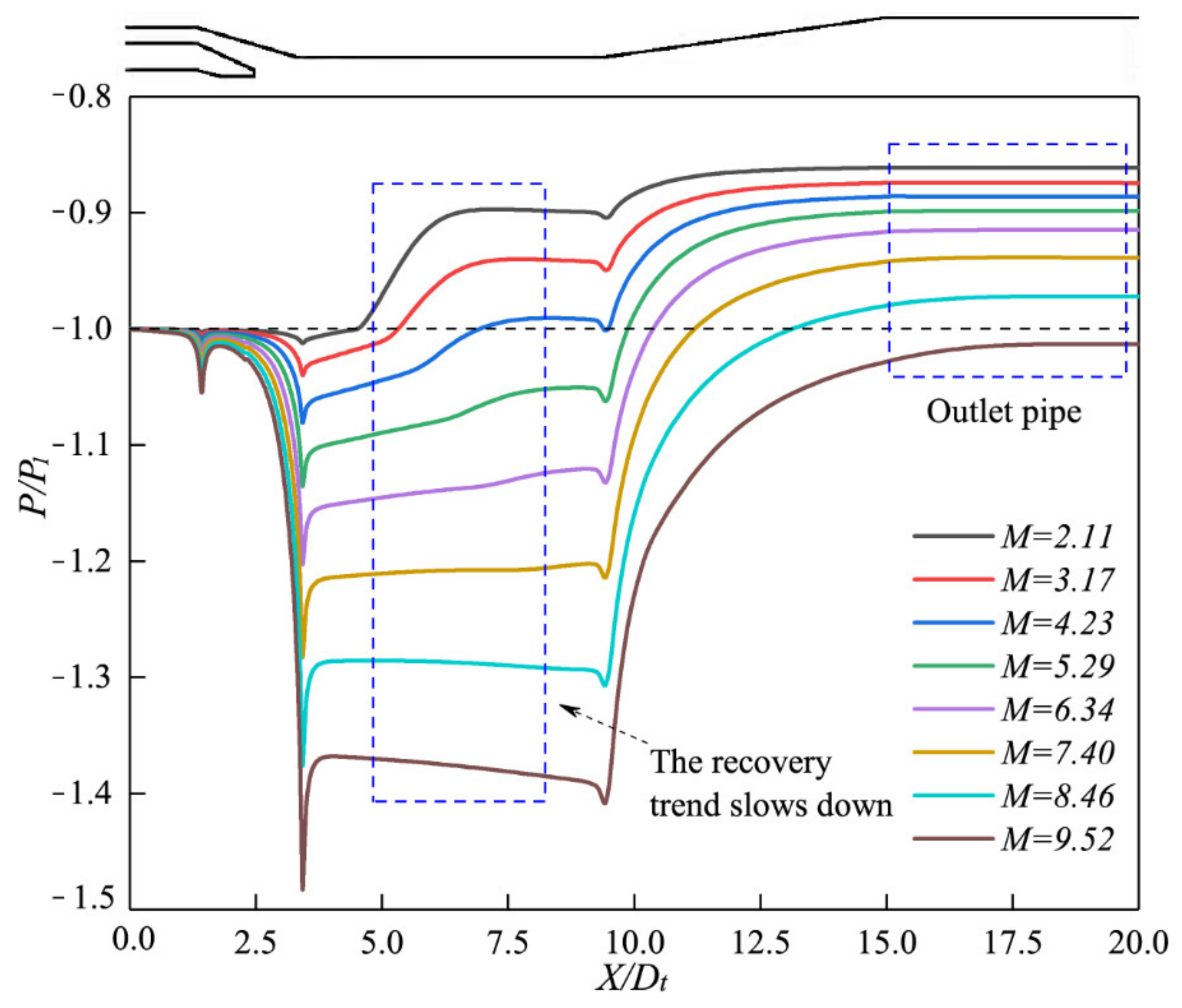
3.3.1. Slurry Pressure Changes

The pressure at the suction is P₁, and the pressure distribution of the slurry is shown in Figure 9. The continuous pressure loss was caused by the shear friction of the low-velocity slurry along the wall. Due to the negative pressure caused by the high-velocity working fluid, the slurry pressure was greatly reduced in the suction chamber. Then, it diffused through the diffuser and finally reached the straight outlet pipe. As the flow ratio increased, the slurry pressure continued to decrease, while the pressure at the throat inlet was greatly reduced. This is mainly because the higher flow rate of the slurry supplied a larger range of velocity and pressure fluctuations [46], resulting in more energy loss. In addition, by comparing the pressure distribution of the outlet pipe, it can be found that when the flow ratio M = 2.11 to 8.46, the outlet pressure Pe of the slurry was greater than the initial pressure P₁ of the slurry. When M = 9.52 and Pe < P₁, the slurry constantly consumed energy in the jet pump, and the high velocity made it difficult for the slurry to obtain energy from the working fluid during the mixing process.

3.3.2. Slurry Velocity Change

The slurry velocity contours of the lengthwise section are shown in Figure 10. With the increase in the flow ratio, the jet core of the slurry became longer and extended downstream from the mixing tube. In summary, the overall velocity of the slurry was apparently increased. The wall velocity distribution of the slurry from nozzle inlet to exit is shown in Figure 11. The slurry velocity reduced because of the wall energy loss; then, it accelerated rapidly to the first peak. In the mixing tube, there was a minimum value of the slurry velocity, and the position where the lowest velocity appeared also moved behind. When M = 7.40, the minimum slurry velocity V_min = 6.33 m/s appeared in the middle sections of the mixing tube, which left sufficient space for the acceleration of the mixed fluid, and then the second peak V_max2 = 7.60 m/s, and the velocity difference between the two phases flows at this time became small. In the diffuser, the kinetic energy was smoothly converted into pressure energy, and then it was stably delivered to the downstream pipeline.

3.4. Mixed Transportation of Two-Phase Flow

To analyze the flow state of the mixed fluid, ten cross-sections from X₁ to X₁₀ were intercepted uniformly along the X direction in the jet pump, which is shown in Figure 12. We took the cross-sections X₃~X₁₀ to draw the velocity profile along this trajectory, as shown in Figure 13. The flow velocity along the trajectory gradually decelerated from the protruding peak when entering the mixing tube, and the jet velocity gradient decreased so that the stratification phenomenon weakened in the middle of the stream. When it reached the outlet of the mixing tube, a good arc-shaped distribution of the mixed fluid was exhibited, and the overall velocity reduction also became more uniform after passing through the diffuser. When the flow rate was quite high, the slurry velocity near the mainstream of the mixing tube appeared to decrease because there was a forward acceleration caused by the working fluid and a reverse pressure gradient between the two-phase flow that interacted [47]. However, in the diffuser, the flow velocity of the tube wall layer was substantially reduced under the high flow rate, which was consistent with the distribution of turbulent kinetic energy in the diffuser.

3.5. Overall Working Performance of the Jet Slurry Pump

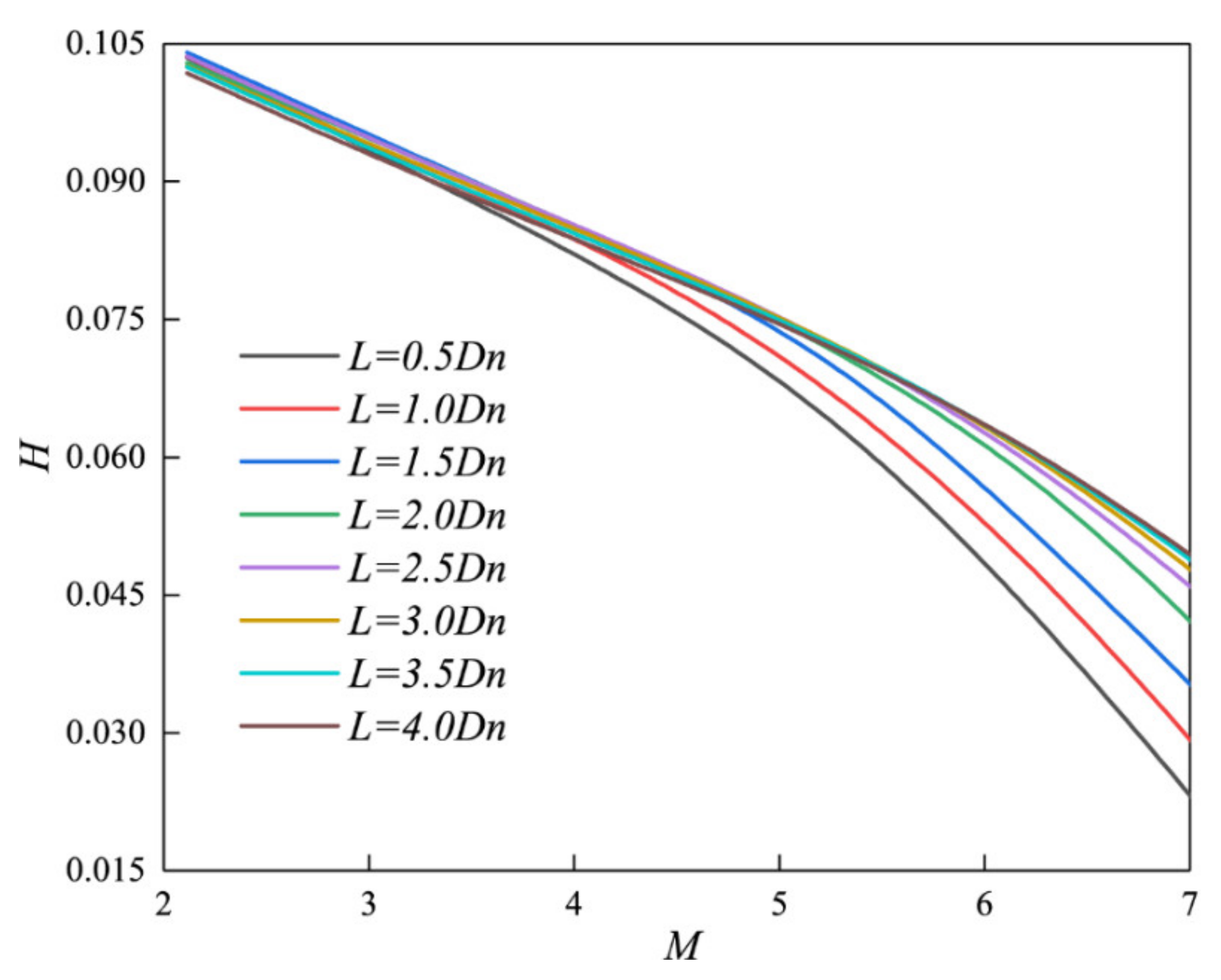
3.5.1. Pressure Ratio H

In Figure 14, the operation curve of the jet slurry pump under different mixing chamber lengths L is shown. As the flow ratio increased, the pressure ratio of the jet slurry pump continuously decreased. The pressure ratio greatly decreased when the flow ratio was high because, at a high flow rate, the velocity of the injected slurry increases faster, and more losses are generated in the suction pipe and the mixing chamber. However, as the length of the mixing chamber L increased, the pressure ratio curve moved up, especially under the condition of a high flow ratio. At the same time, there was an approximate parabolic mathematical relationship between the pressure ratio and the flow ratio [1]. In this study, the data of L = 3.5D_n were selected for fitting, and the function of H regarding M could be obtained:

$$H=0.113-3.92\times {10}^{-3}·M-7.449\times {10}^{-4}·M^2$$

(10)

This formula can be used for the selection calculation of jet slurry pumps. It has certain reference significance for jet pumps with specific requirements.

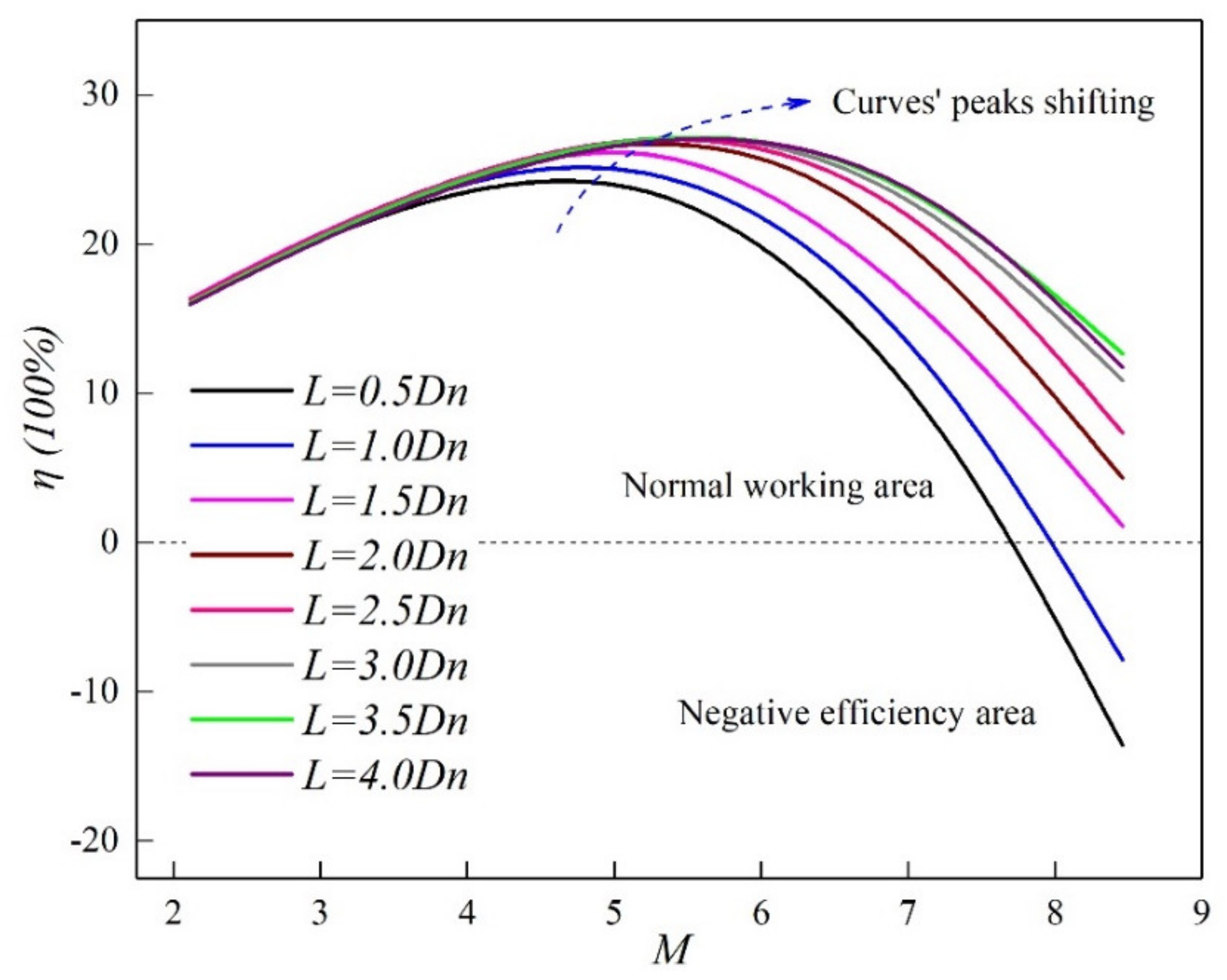
3.5.2. Efficiency of Jet Slurry Pump

The efficiency curve at different mixing chamber lengths is shown in Figure 15. The mixing chamber length and ejection flow ratio of the jet slurry pump had a significant influence on the working performance. As the flow ratio increased, the efficiency showed a parabolic trend with peak efficiency and negative efficiency regions. Due to the absence of moving parts and low energy conversion rate, the overall efficiency of the jet slurry pump did not exceed 30%, but there was a high-efficiency flow ratio section. As the length of the mixing chamber increased, the efficiency of the jet pump gradually increased, the peak moved to the right, and the high-efficiency area was available at a higher flow ratio. There is an optimal length of the mixing chamber. In this study, L = 3.5D_n was selected, the efficiency curve was relatively broad, and the maximum efficiency was η_max = 27.6%. However, once the flow ratio is too high, the jet slurry pump will enter a reverse suction area with negative efficiency [48], due to the fact that the slurry flow rate is too high to replace the working fluid in the mainstream, and a large amount of momentum is lost in the mixing process.

4. Conclusions

The present study attempts to illuminate the flow details of a jet pump used for slurry transporting by computational fluid dynamics methods, for the purpose of guiding the design and application in the dredging field. The results show that the jet pump underwent rapid jet decay, displayed a strong pressure attenuation in the throat and has a limited range of efficient operation.

(1)

The mainstream and the secondary jet mixed strongly in the suction chamber, and gradually mixed well in the throat tube. As the flow ratio increased, the jet pressures along the axis showed a downward trend, and the turbulent kinetic energy in the mixing tube dropped sharply.

(2)

As the flow ratio increased, the wall pressure continued to decline. When the outlet pressure dropped below the suction pressure, the jet slurry pump was difficult to operate normally.

(3)

The efficiency was greatly affected by the mixing chamber length and flow ratio and presented a parabolic shape. When L = 3.5D_n, the best comprehensive performance of the jet slurry pump was achieved, which could reach 27.6%.

(4)

Due to the lack of research on jet slurry pumps, a specific structure model was devised and analyzed in this paper. In future work, the influence of structural parameters and different slurry concentrations will be taken into account.

References

1. Bi, Z.Y. Research on Efficiency Optimization and Control for Dredging Slurry Pipeline Transport System. Ph.D. Thesis, Zhejiang University, Hangzhou, China, 2008. Available online: https://kns.cnki.net/KCMS/detail/detail.aspx?dbname=CDFD0911&filename=2009033175.nh (accessed on 1 April 2008).
2. Boor, M.O. Production Optimization; IHC Company: Kinderdijk, The Netherlands, 2005. [Google Scholar]
3. Miedema, S.A. Slurry Transport Fundamentals. In A Historical Overview & The Delft Head Loss and Limit Deposit Velocity Framework; Delft University of Technology: Delft, The Netherlands, 2016; pp. 107–118. [Google Scholar]
4. Panevnik, A.V. Determination of Hydraulic Losses in the Setting of a Well Jet Pump. Chem. Pet. Eng. 2001, 37, 368–369. [Google Scholar] [CrossRef]
5. Meakhail, A.T.; Zien, Y.; Elsallak, M.; AbdelHady, S. Experimental study of the effect of some geometric variables and number of nozzles on the performance of a subsonic air—Air ejector. Proc. Inst. Mech. Eng. Part A J. Power Energy 2008, 222, 809–818. [Google Scholar] [CrossRef]
6. Everitt, P.; Riffat, S.B. Steam jet ejector system for vehicle air conditioning. Int. J. Ambient. Energy 1999, 20, 14–20. [Google Scholar] [CrossRef]
7. Jafarian, A.; Azizi, M.; Forghani, P. Experimental and numerical investigation of transient phenomena in vacuum ejectors. Energy 2016, 102, 528–536. [Google Scholar] [CrossRef]
8. Wang, J.; Xu, S.J.; Cheng, H.Y.; Ji, B.; Zhang, J.Q.; Long, X.P. Experimental investigation of cavity length pulsation characteristics of jet pumps during limited operation stage. Energy 2018, 163, 61–73. [Google Scholar] [CrossRef]
9. Aphornratana, S.; Eames, I.W. A small capacity steam-ejector refrigerator: Experimental investigation of a system using ejector with movable primary nozzle. Int. J. Refrig. 1997, 20, 352–358. [Google Scholar] [CrossRef]
10. Gogate, P.R. Cavitational reactors for process intensification of chemical processing applications: A critical review. Chem. Eng. Process. Process. Intensif. 2008, 47, 515–527. [Google Scholar] [CrossRef]
11. Alperin, M.; Wu, J.-J. Thrust Augmenting Ejectors, Part, I. AIAA J. 1983, 21, 1428–1436. [Google Scholar] [CrossRef]
12. Beithou, N.; Aybar, H.S. High-Pressure Steam-Driven Jet Pump—Part II: Parametric Analysis. J. Eng. Gas Turbines Power 2001, 123, 701–706. [Google Scholar] [CrossRef]
13. Xiao, L.Z.; Long, X.P.; Li, L.; Xu, M.; Wu, N.; Wang, Q. Movement characteristics of fish in a jet fish pump. Ocean Eng. 2015, 108, 480–492. [Google Scholar] [CrossRef]
14. Balamurugan, S.; Lad, M.D.; Gaikar, V.G.; Patwardhan, A.W. Hydrodynamics and mass transfer characteristics of gas–liquid ejectors. Chem. Eng. J. 2007, 131, 83–103. [Google Scholar] [CrossRef]
15. Yang, X.; Long, X.; Kang, Y. Effect of diffuser structure and throat length on jet pump performance. J. Harbin Inst. Technol. 2014, 46, 111–115. [Google Scholar]
16. Banasiak, K.; Palacz, M.; Hafner, A.; Buliński, Z.; Smołka, J.; Nowak, A.J.; Fic, A. A CFD-based investigation of the energy performance of two-phase R744 ejectors to recover the expansion work in refrigeration systems: An irreversibility analysis. Int. J. Refrig. 2014, 40, 328–337. [Google Scholar] [CrossRef]
17. Havelka, P.; Linek, V.; Sinkule, J.; Zahradník, J.; Fialova, M. Effect of the ejector configuration on the gas suction rate and gas hold-up in ejector loop reactors. Chem. Eng. Sci. 1997, 52, 1701–1713. [Google Scholar] [CrossRef]
18. Yang, X.L.; Long, X.P.; Kang, Y.; Xiao, L.Z. Application of Constant Rate of Velocity or Pressure Change Method to Improve Annular Jet Pump Performance. Int. J. Fluid Mach. Syst. 2013, 6, 137–143. [Google Scholar] [CrossRef] [Green Version]
19. Saker, A.A.; Hassan, H.Z. Study of the Different Factors That Influence Jet Pump Performance. Open J. Fluid Dyn. 2013, 3, 44–49. [Google Scholar] [CrossRef] [Green Version]
20. Besagni, G.; Inzoli, F. Computational fluid-dynamics modeling of supersonic ejectors: Screening of turbulence modeling approaches. Appl. Therm. Eng. 2017, 117, 122–144. [Google Scholar] [CrossRef]
21. Mallela, R.; Chatterjee, D. Numerical investigation of the effect of geometry on the performance of a jet pump. Proc. Inst. Mech. Eng. Part C J. Mech. Eng. Sci. 2011, 225, 1614–1625. [Google Scholar] [CrossRef]
22. Girgidov, A.D. Efficiencies of Jet Pumps. Power Technol. Eng. 2015, 48, 366–370. [Google Scholar] [CrossRef]
23. Banasiak, K.; Hafner, A.; Andresen, T. Experimental and numerical investigation of the influence of the two-phase ejector geometry on the performance of the R744 heat pump. Int. J. Refrig. 2012, 35, 1617–1625. [Google Scholar] [CrossRef]
24. Long, X.; Han, N.; Chen, Q. Influence of nozzle exit tip thickness on the performance and flow field of jet pump. J. Mech. Sci. Technol. 2008, 22, 1959–1965. [Google Scholar] [CrossRef]
25. Yang, X.L.; Long, X.P. Numerical investigation on the jet pump performance based on different turbulence models. IOP Conf. Ser. Earth Environ. Sci. 2012, 15, 052019. [Google Scholar] [CrossRef]
26. Kumar, R.S.; Kumaraswamy, S.; Mani, A. Experimental investigations on a two-phase jet pump used in desalination systems. Desalination 2006, 204, 437–447. [Google Scholar] [CrossRef]
27. Yasmin, H.; Iqbal, N.; Tanveer, A. Engineering Applications of Peristaltic Fluid Flow with Hall Current, Thermal Deposition and Convective Conditions. Mathematics 2020, 8, 1710. [Google Scholar] [CrossRef]
28. Yasmin, H.; Iqbal, N. Convective Mass/Heat Analysis of an Electroosmotic Peristaltic Flow of Ionic Liquid in a Symmetric Porous Microchannel with Soret and Dufour. Math. Probl. Eng. 2021, 2021, 1–14. [Google Scholar] [CrossRef]
29. Iqbal, N.; Yasmin, H.; Kometa, B.K.; Attiya, A.A. Effects of Convection on Sisko Fluid with Peristalsis in an Asymmetric Channel. Math. Comput. Appl. 2020, 25, 52. [Google Scholar] [CrossRef]
30. Iqbal, N.; Yasmin, H.; Bibi, A.; Attiya, A.A. Peristaltic motion of Maxwell fluid subject to convective heat and mass conditions. Ain Shams Eng. J. 2021, 12, 3121–3131. [Google Scholar] [CrossRef]
31. Du, W.; Luo, L.; Wang, S.; Liu, J.; Sunden, B. Numerical investigation of flow field and heat transfer characteristics in a latticework duct with jet cooling structures. Int. J. Therm. Sci. 2020, 158, 106553. [Google Scholar] [CrossRef]
32. Zhou, L.; Wang, W.; Hang, J.; Shi, W.; Yan, H.; Zhu, Y. Numerical Investigation of a High-Speed Electrical Submersible Pump with Different End Clearances. Water 2020, 12, 1116. [Google Scholar] [CrossRef] [Green Version]
33. Engin, T.; Gur, M. Performance Characteristics of a Centrifugal Pump Impeller With Running Tip Clearance Pumping Solid-Liquid Mixtures. J. Fluids Eng. 2001, 123, 532–538. [Google Scholar] [CrossRef]
34. Winoto, S.H.; Li, H.; Shah, D.A. Efficiency of Jet Pumps. J. Hydraul. Eng. 2000, 126, 150–156. [Google Scholar] [CrossRef]
35. Long, X.P.; Zhang, J.Q.; Wang, Q.Q.; Xiao, L.Z.; Xu, M.S.; Lyu, Q.; Ji, B. Experimental investigation on the performance of jet pump cavitation reactor at different area ratios. Exp. Therm. Fluid Sci. 2016, 78, 309–321. [Google Scholar] [CrossRef]
36. Long, X.P.; Wang, J.; Zhang, J.Q.; Ji, B. Experimental investigation of the cavitation characteristics of jet pump cavitation reactors with special emphasis on negative flow ratios. Exp. Therm. Fluid Sci. 2018, 96, 33–42. [Google Scholar] [CrossRef]
37. El-Sawaf, I.A.; Halawa, M.A.; Younes, M.A.; Teaima, I.R. Study of the different parameters that influence on the performance of water jet pump. In Proceedings of the Fifteenth International Water Technology Conference, Alexandria, Egypt, 15 July 2011; Volume 15. Available online: http://citeseerx.ist.psu.edu/viewdoc/summary?doi=10.1.1.302.842 (accessed on 1 November 2013).
38. ANSYS Fluent Theory Guide 15. Inc. ANSYS. 2013. Available online: https://www.ansys.com/products/fluids/ansys-fluent (accessed on 1 November 2013).
39. Lucas, C.; Rusche, H.; Schroeder, A.; Koehler, J. Numerical investigation of a two-phase CO2 ejector. Int. J. Refrig. 2014, 43, 154–166. [Google Scholar] [CrossRef]
40. Xu, M.S.; Long, X.P.; Yang, X.L. Effects of nozzle location on new type annular jet pump performance. J. Drain. Irrig. Mach. Eng. 2014, 32, 563–566. [Google Scholar]
41. Giacomelli, F.; Mazzelli, F.; Banasiak, K.; Hafner, A.; Milazzo, A. Experimental and computational analysis of a R744 flashing ejector. Int. J. Refrig. 2019, 107, 326–343. [Google Scholar] [CrossRef] [Green Version]
42. Sriveerakul, T.; Aphornratana, S.; Chunnanond, K. Performance prediction of steam ejector using computational fluid dynamics: Part 1. Validation of the CFD results. Int. J. Therm. Sci. 2007, 46, 812–822. [Google Scholar] [CrossRef]
43. Yu, J.L.; Guo, X.H.; Hu, X.S. Experimental research of liquid-liquid &gas jet pump. Chem. Ind. Eng. 2001, 2, 103–108. Available online: https://kns.cnki.net/kcms/detail/detail.aspx?dbcode=CJFD&dbname=CJFD2001&filename=HXGY200102007&uniplatform=NZKPT&v=2AVd12xm9-ZDIuYn7z-nf680zWyky_9HVOeNxiXCj09_9Wh6sQS2GRF6Z_eoQcI3 (accessed on 1 April 2001).
44. Long, X.P.; Cheng, H.G.; Yang, X.L.; Xiao, L.Z. Numerical and experimental investigations on super-large area-ratio jet pumps. J. Drain. Irrig. Mach. Eng. 2012, 30, 379–383. [Google Scholar]
45. Zhao, Y.H. Numerical Simulation for Hyrodynamic Characteristics and Internal Flow Field of Jet Pump. Master’s Thesis, Northeast Petroleum University, Daqing, China, 2012. Available online: https://kns.cnki.net/KCMS/detail/detail.aspx?dbname=CMFD201301&filename=1012432055.nh (accessed on 23 March 2012).
46. Wu, Y.; Zhao, H.; Zhang, C.; Wang, L.; Han, J. Optimization analysis of structure parameters of steam ejector based on CFD and orthogonal test. Energy 2018, 151, 79–93. [Google Scholar] [CrossRef]
47. Xu, M.S.; Yang, X.L.; Long, X.P.; Lü, Q. Large eddy simulation of turbulent flow structure and characteristics in an annular jet pump. J. Hydrodyn. 2017, 29, 702–715. [Google Scholar] [CrossRef]
48. Liu, Y. Study on Performance of the Steam Ejector Used for Low Pressure Gas well Deliquification. Master’s Thesis, China University of Petroleum, Beijing, China, 2018. Available online: https://kns.cnki.net/KCMS/detail/detail.aspx?dbname=CMFD202001&filename=1019927532.nh (accessed on 1 May 2018).
Figure 1. Schematic diagram and main parameters of the jet pump.
Processes 09 02053 g001
Figure 2. The 3D computational domain and boundary conditions of the jet pump.
Processes 09 02053 g002
Figure 3. Grid of computational domain and cross-sections.
Processes 09 02053 g003
Figure 4. Comparison of the CFD results and the experimental data [43]. (The data points were extracted from the reference).
Processes 09 02053 g004
Figure 5. Axial pressure distribution from nozzle inlet to exit (M = 2.11, 3.17, 4.23, 5.29, 6.34, 7.40, 8.46, 9.52).
Processes 09 02053 g005
Figure 6. Turbulent kinetic energy distribution of lengthwise section (M = 2.11, 3.17, 4.23, 5.29, 6.34, 7.40, 8.46, 9.52).
Processes 09 02053 g006
Figure 7. Turbulent kinetic energy distribution of the shaft axis from nozzle inlet to exit (M = 2.11, 3.17, 4.23, 5.29, 6.34, 7.40, 8.46, 9.52).
Processes 09 02053 g007
Figure 8. Velocity distribution of shaft axis from nozzle inlet to exit (M = 2.11, 3.17, 4.23, 5.29, 6.34, 7.40, 8.46, 9.52).
Processes 09 02053 g008
Figure 9. Wall pressure distribution of slurry from nozzle inlet to exit (M = 2.11, 3.17, 4.23, 5.29, 6.34, 7.40, 8.46, 9.52).
Processes 09 02053 g009
Figure 10. Slurry velocity contours of lengthwise section (M = 2.11, 3.17, 4.23, 5.29, 6.34, 7.40, 8.46, 9.52).
Processes 09 02053 g010
Figure 11. Wall velocity distribution of slurry from nozzle inlet to exit (M = 2.11, 3.17, 4.23, 5.29, 6.34, 7.40, 8.46, 9.52).
Processes 09 02053 g011
Figure 12. Schematic diagram of ten cross-section positions (X1-X1 to X10-X10).
Processes 09 02053 g012
Figure 13. Velocity profile of cross-sections X3-X3~X10-X10 (M = 2.11, 3.17, 4.23, 5.29, 6.34, 7.40, 8.46, 9.52).
Processes 09 02053 g013
Figure 14. Operation curves at different mixing chamber lengths (L = 0.5, 1.0, 1.5, 2.0, 2.5, 3.0, 3.5, 4.0 Dn).
Processes 09 02053 g014
Figure 15. Efficiency curves at different mixing chamber lengths (L = 0.5, 1.0, 1.5, 2.0, 2.5, 3.0, 3.5, 4.0 Dn).
Processes 09 02053 g015