
Real-Time Dynamic Carbon Content Prediction Model for Second Blowing Stage in BOF Based on CBR and LSTM

Abstract
:1. Introduction
2. Converter Steelmaking Process
2.1. Smelting
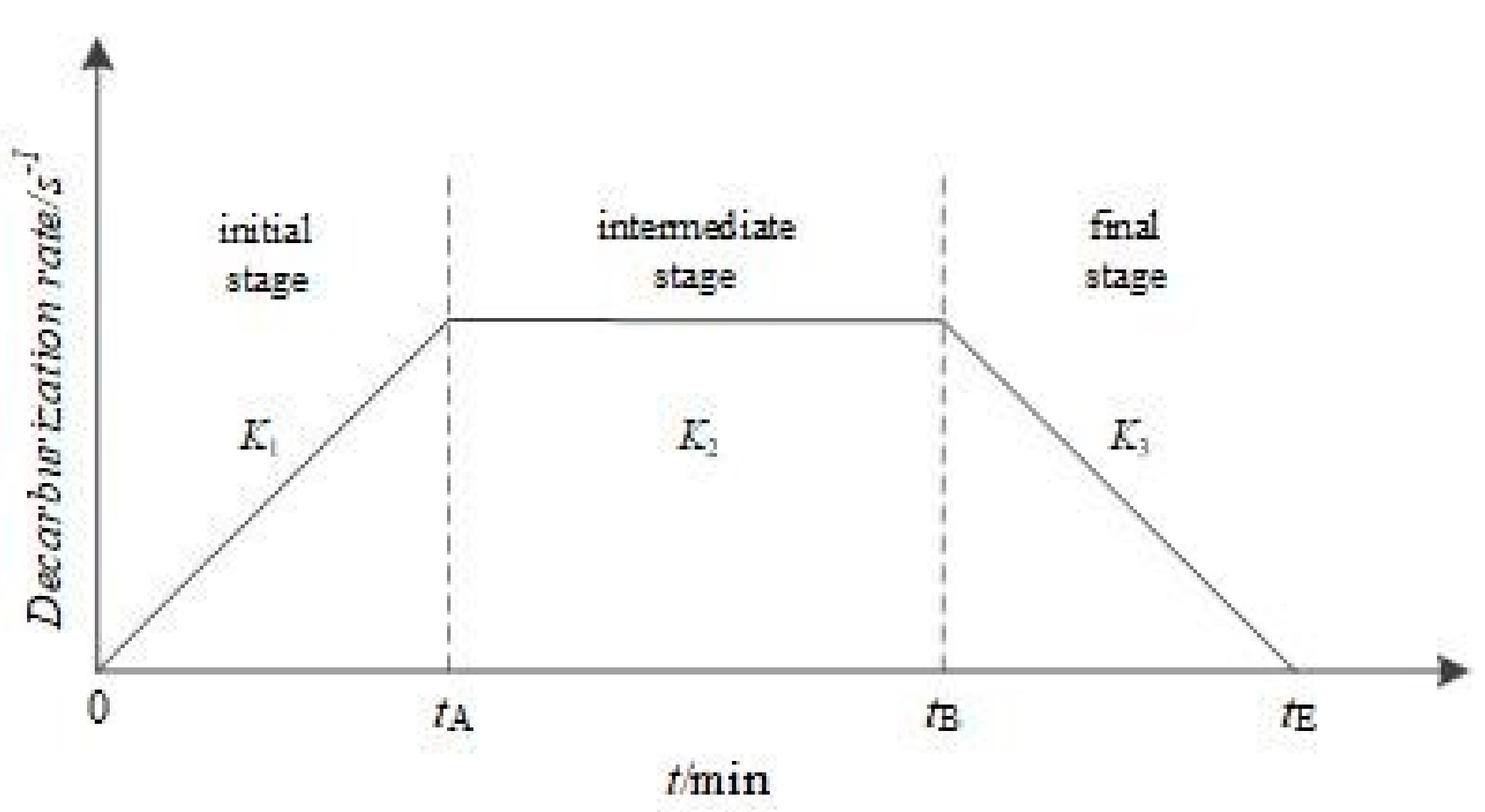
2.2. Decarburisation
2.3. Process Parameters for Converter Steelmaking
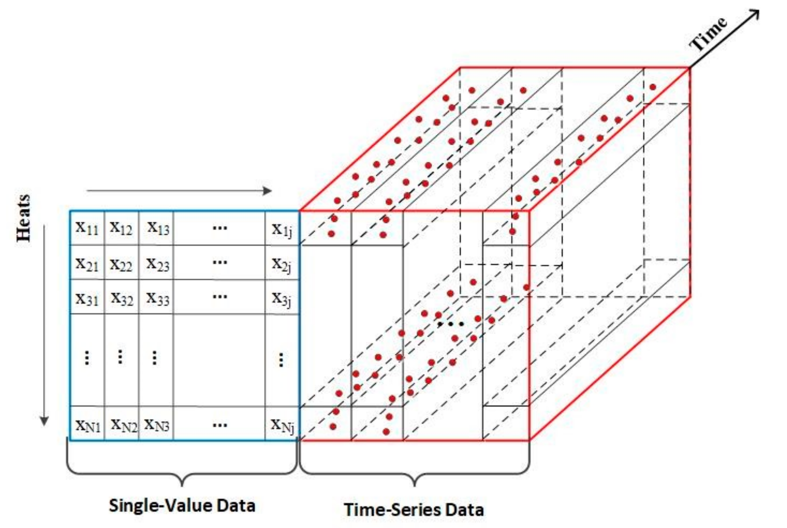
- (1)
- Single-value data
- (2)
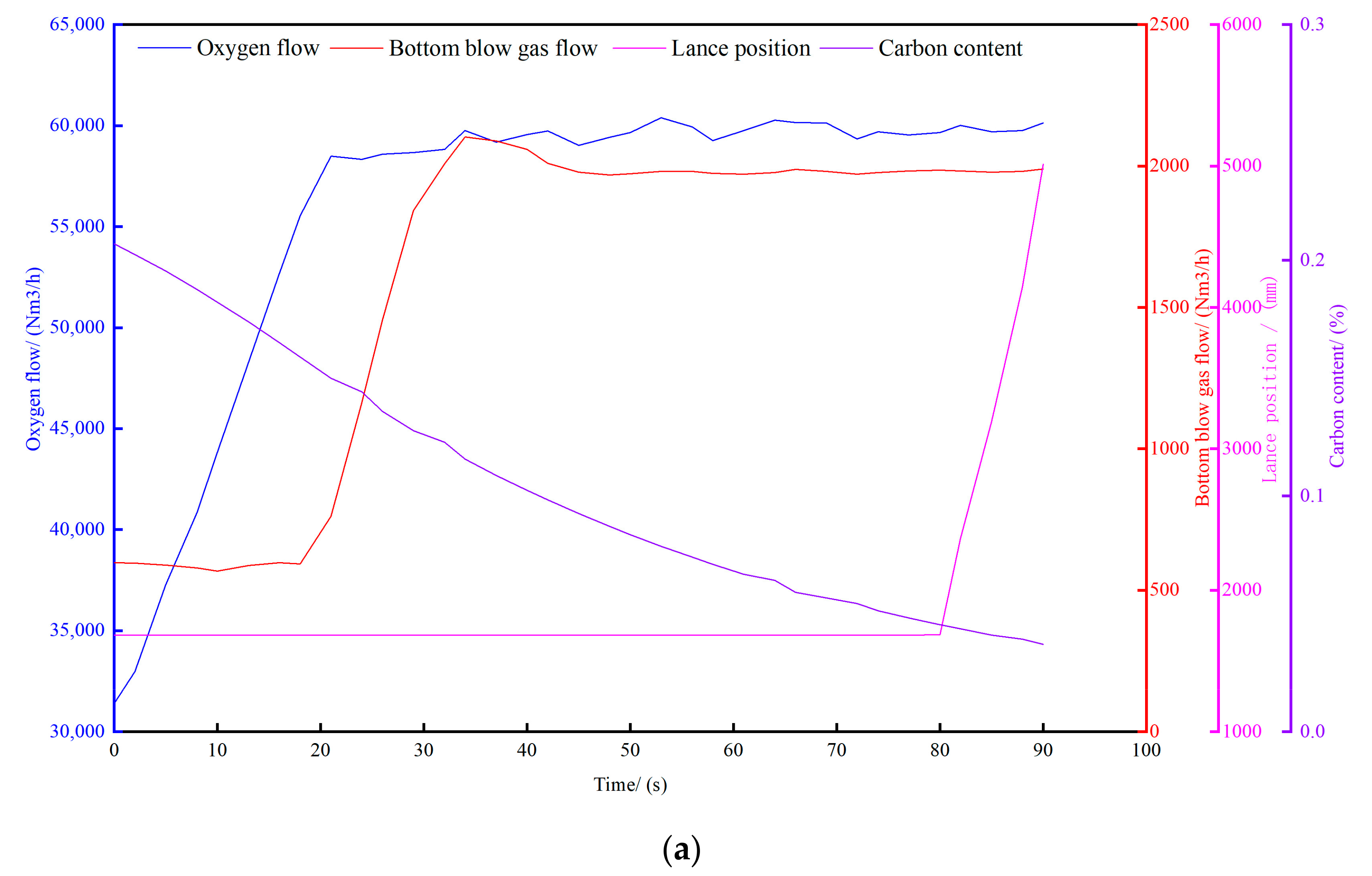
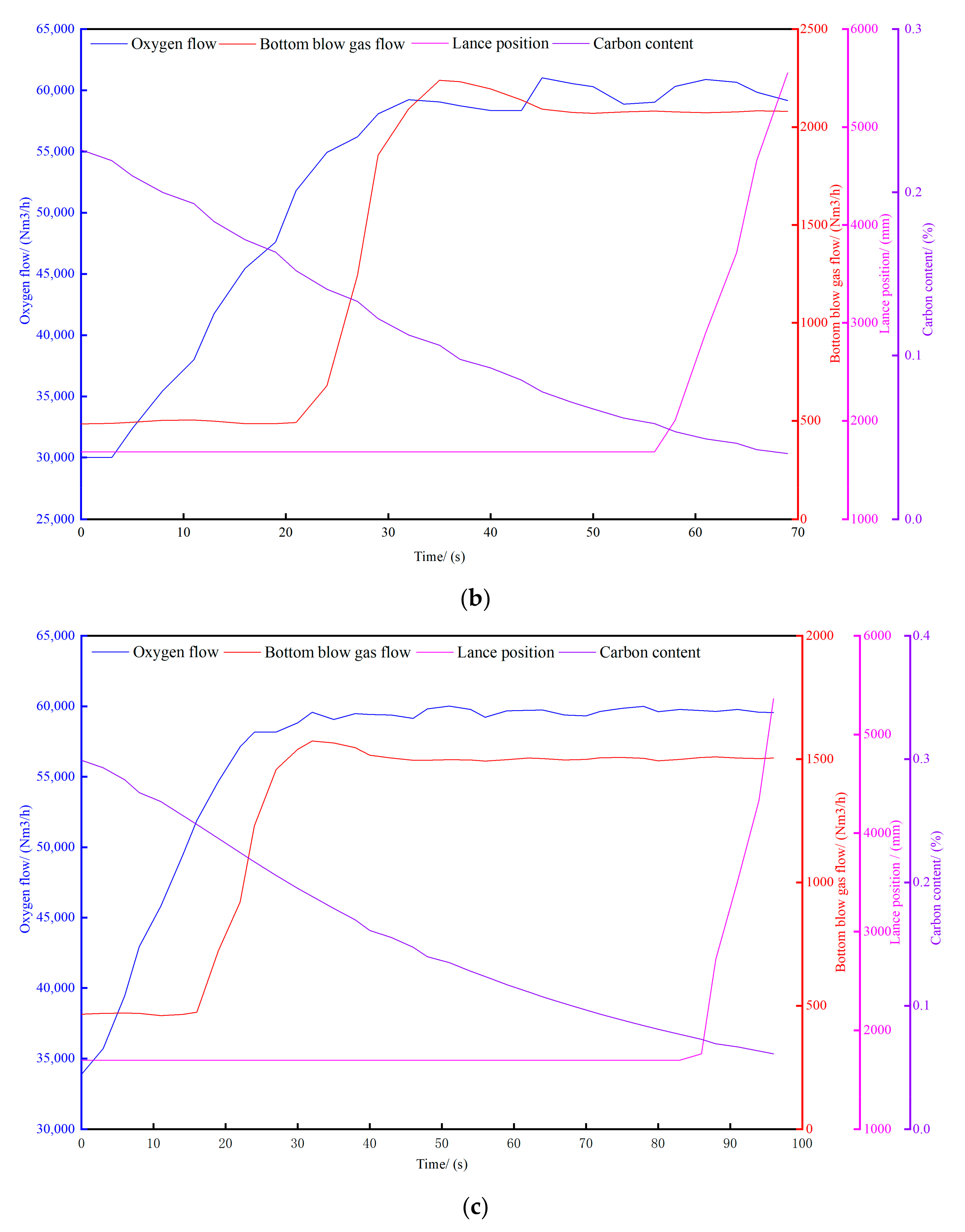
- Time-series data
3. Methodology
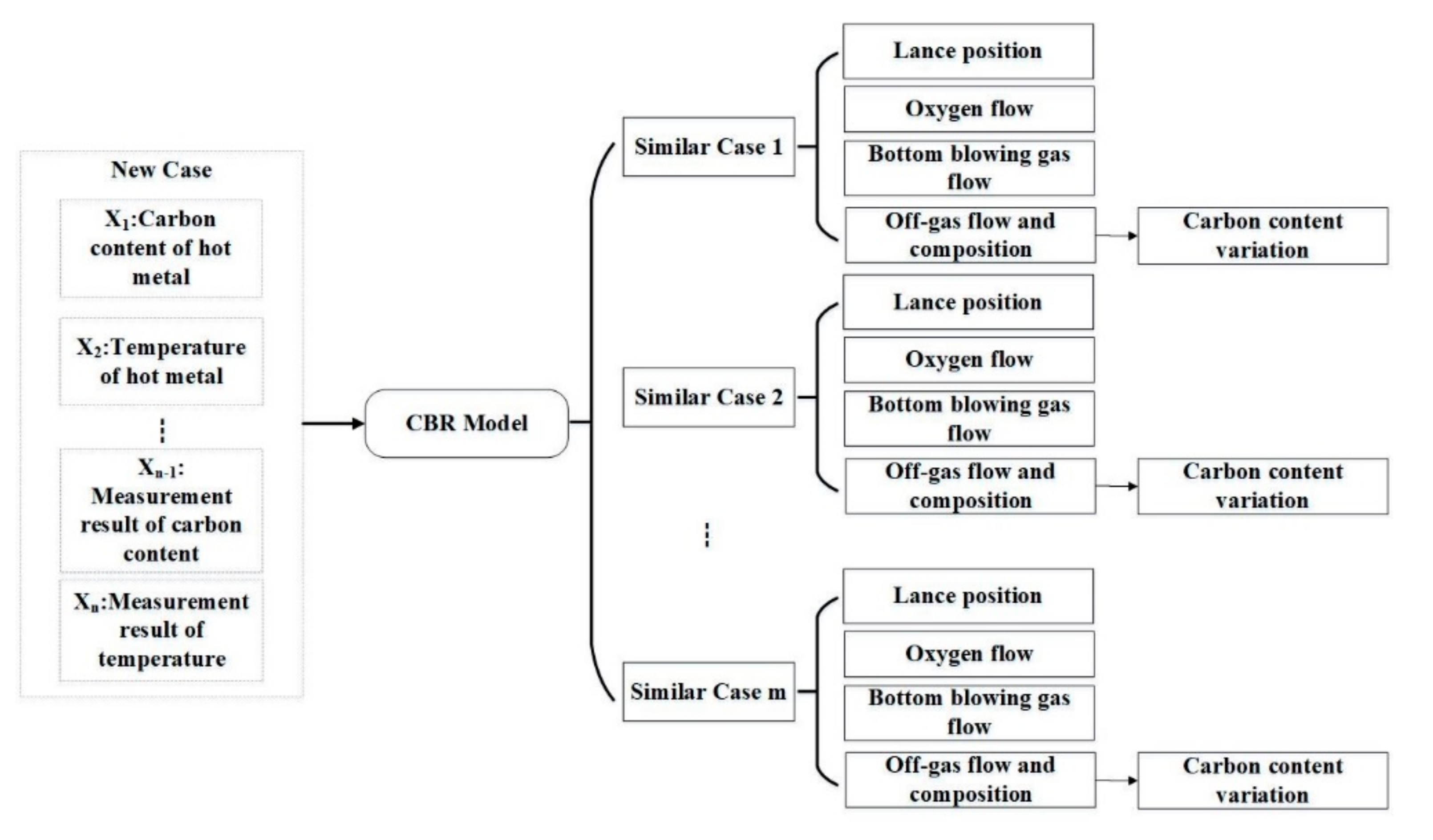
3.1. Case-Based Reasoning
3.2. Long Short-Term Memory Neural Network
3.3. Prediction Model Bsaed on off-Gas Analysis
- (1)
- Carbon integral model
- (2)
- Exponential decay model
3.4. Principles of Model
4. Model Application Examples
4.1. Datasets
4.2. Similar Case Retrieval
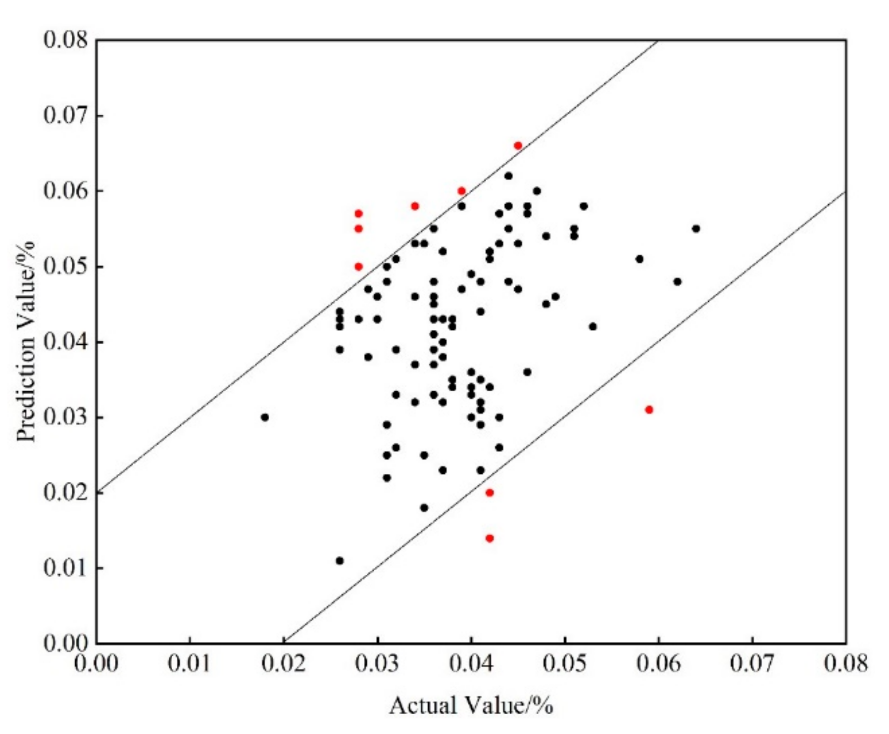
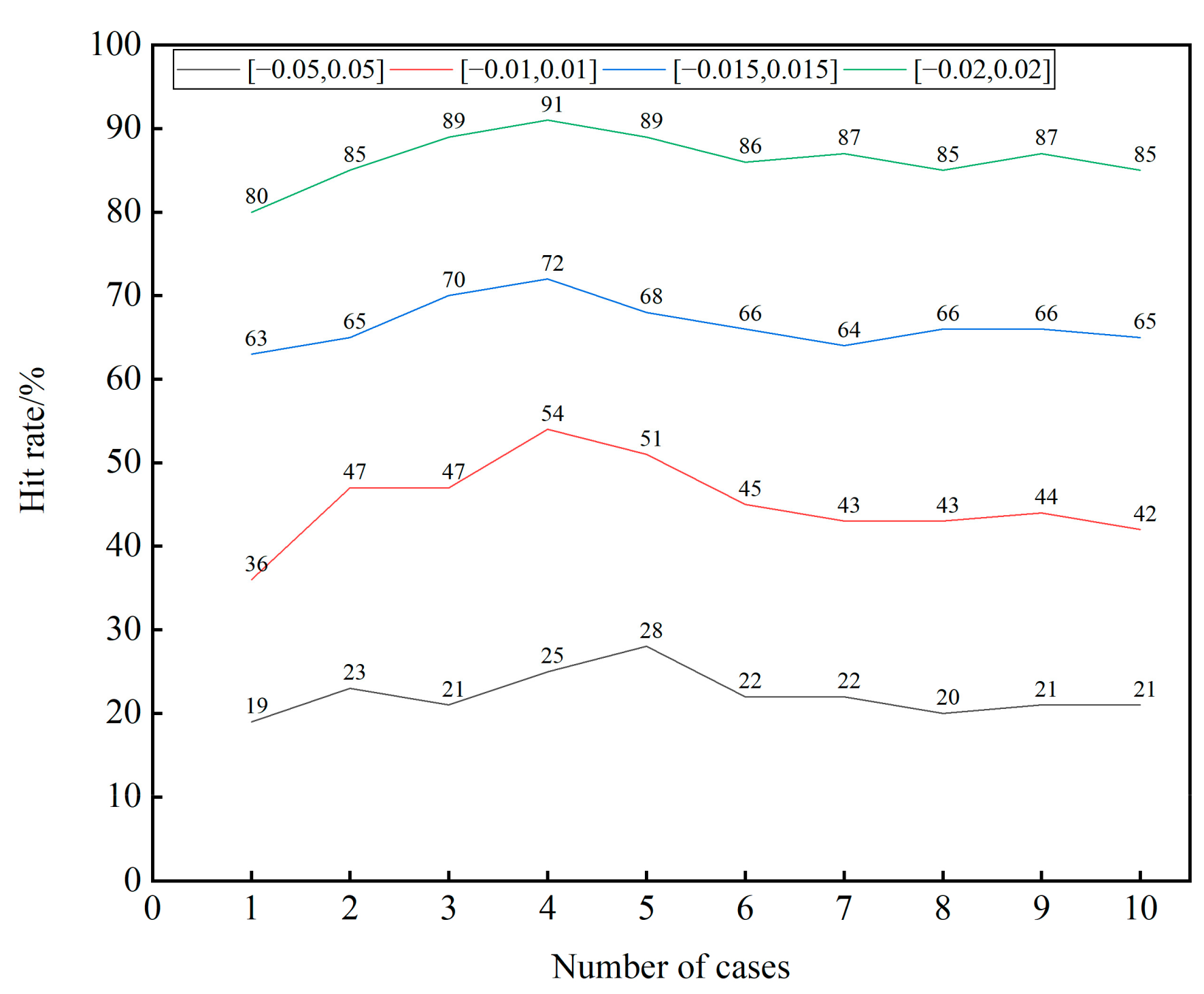
4.3. Model Training and Validation
5. Conclusions
- (1)
- The dynamic prediction model to predict the temperature of molten steel in the second blowing stage.
- (2)
- The dynamic prediction model to predict the temperature and carbon content of molten steel in the whole blowing stage.
Author Contributions
Funding
Institutional Review Board Statement
Informed Consent Statement
Data Availability Statement
Conflicts of Interest
References
- Han, M.; Wang, X.Z. BOF oxygen control by mixed case retrieve and reuse CBR. IFAC Pro. Vol. 2011, 44, 3575–3580. [Google Scholar] [CrossRef] [Green Version]
- Wang, X.; Han, M. Causality-based CBR model for static control of converter steelmaking. J. Dalian Univ. Technol. 2011, 51, 593–598. (In Chinese) [Google Scholar]
- Park, T.C.; Kim, B.S.; Kim, T.Y.; Jin, B.; Yeo, Y.K. Comparative Study of Estimation Methods of the Endpoint Temperature in Basic Oxygen Furnace Steelmaking Process with Selection of Input Parameters. Korean J. Met. Mater. 2018, 56, 813–821. [Google Scholar] [CrossRef]
- Gao, C.; Shen, M.G.; Wang, L.D. End-point Prediction of BOF Steelmaking Based on Wavelet Transform Based Weighted TSVR. In Proceedings of the 37th Chinese Control Conference, Wuhan, China, 25–27 July 2018. [Google Scholar]
- Gao, C.; Shen, M.G.; Liu, X.P.; Wang, L.D.; Chen, M. End-point Prediction of BOF Steelmaking Based on KNNWTSVR and LWOA. Trans. Trans. Indian Inst. Met. 2018, 72, 257–270. [Google Scholar] [CrossRef]
- Li, W.; Wang, X.C.; Wang, X.S.; Wang, H. Endpoint Prediction of Bof Steelmaking Based on BP Neural Network Combined with Improved PSO. Chem. Eng. Trans. 2016, 51, 475–480. [Google Scholar]
- Han, M.; Liu, C. Endpoint prediction model for basic oxygen furnace steel-making based on membrane algorithm evolving extreme learning machine. Appl. Soft Comput. 2014, 19, 430–437. [Google Scholar] [CrossRef]
- Zhou, M.C.; Zhao, Q.; Chen, Y.R. Endpoint prediction of BOF by flame spectrum and furnace mouth image based on fuzzy support vector machine. Optik 2018, 178, 575–581. [Google Scholar] [CrossRef]
- Chen, J.; Wang, J. Endpoint prediction method for steelmaking based on multi-task learning. J. Comput. Appl. 2017, 37, 889–895. (In Chinese) [Google Scholar]
- Liang, Y.R.; Wang, H.B.; Xu, A.J.; Tian, N.Y. A Two-step Case-based Reasoning Method Based on Attributes Reduction for Predicting the Endpoint Phosphorus Content. ISIJ Int. 2015, 55, 1035–1043. [Google Scholar] [CrossRef] [Green Version]
- Wang, H.B.; Xu, A.J.; Al, L.X.; Tian, N.Y.; Du, X. An Integrated CBR Model for Predicting Endpoint Temperature of Molten Steel in AOD. ISIJ Int. 2012, 52, 80–86. [Google Scholar] [CrossRef] [Green Version]
- Liu, H.; Wu, Q.; Wang, B.; Xiong, X. BOF steelmaking endpoint real-time recognition based on flame multi-scale color difference histogram features weighted fusion method. In Proceedings of the 35th Chinese Control Conference, Chengdu, China, 27–29 July 2016. [Google Scholar]
- Luo, T.; Liu, H.; Wu, Q.S.; Wang, B. Prediction method of carbon content in BOF endpoint based on convolutional neural network. Inf. Tech. 2018, 42, 150–155. (In Chinese) [Google Scholar]
- Yan, L.T.; Li, M.; Yang, D.Y. Prediction of Carbon Content at End Point Based on GA-KPLSR in Converters. Control Eng. China 2017, 24, 923–926. [Google Scholar]
- Ahmad, I.; Kano, M.; Hasebe, S.; Kitada, H.; Murata, N. Prediction of Molten Steel Temperature in Steel Making Process with Uncertainty by Integrating Gray-Box Model and Bootstrap Filter. J. Chem. Eng. Japan 2014, 47, 827–834. [Google Scholar] [CrossRef] [Green Version]
- Lv, W. A Novel Process Modeling Method for Steel Sulphur Content Soft Sensing during Ladle Furnace Steel Refining. ISIJ Int. 2019, 59, 1276–1286. [Google Scholar] [CrossRef]
- Okura, T.; Ahmad, I.; Kano, M.; Hasebe, S.; Kitada, H.; Murata, N. High-Performance Prediction of Molten Steel Temperature in Tundish through Gray-Box Model. ISIJ Int. 2013, 53, 76–80. [Google Scholar] [CrossRef] [Green Version]
- Yue, F.; Bao, Y.P.; Cui, H.; Gao, S.Y.; Li, B.H.; Zhang, J. Sub-lance control-based predication model for BOF end-point. Steelmaking 2009, 25, 38–59. [Google Scholar]
- Han, M.; Zhao, Y. Dynamic control model of BOF steelmaking process based on ANFIS and robust relevance vector machine. Expert Syst. Appl. 2011, 38, 14786–14798. [Google Scholar] [CrossRef]
- Wang, X.Z.; Xing, J.; Dong, J.; Wang, Z.S. Data driven based endpoint carbon content real time prediction for BOF steelmaking. In Proceedings of the 36th Chinese Control Conference, Dalian, China, 26–28 July 2017. [Google Scholar]
- Hu, Z.G.; He, P.; Liu, L.; Tan, M.X. Continuous Determination of Bath Carbon in BOF by Off-gas Analysis. Res. Iron Steel 2003, 31, 12–15. [Google Scholar]
- Hu, Z.G.; He, P.; Liu, L.; Tan, M.X. Continuous Determination of Bath Temperature in BOF by Off-gas Analysis. In Proceedings of the 5th CSM Annual Steelmaking Conference Proceedings, Congqing, China, 22–24 April 2003. [Google Scholar]
- Liu, K.; Liu, L.; He, P.; Liu, W. A new algorithm of endpoint carbon content of BOF based on of off-gas analysis. Steelmaking 2009, 25, 33–37. [Google Scholar]
- Wang, X.H.; Liu, J.Z.; Liu, F.G. Technological progress of BOF steelmaking in period of development mode transition. Steelmaking 2017, 33, 1–55. [Google Scholar]
- Liao, D.S.; Sun, S.; Waterfall, S.; Boylan, K.; Pyke, N.; Holdridge, D. Integrated KOBM Steelmaking Process Control. In Proceedings of the 6th International Steelmaking Science and Technology Conference, Beijing, China, 12–14 May 2015. [Google Scholar]
- Lin, W.H.; Jiao, S.Q.; Sun, J.K.; Liu, M.; Su, X.; Liu, Q. Modified exponential model for carbon prediction in the end blowing stage of basic oxygen furnace converter. Chin. J. Eng. 2020, 42, 854–861. [Google Scholar]
- Sala, D.A.; Jalalvand, A.; Deyne, Y.D.; Manners, E. Multivariate Time Series for Data-Driven Endpoint Prediction in the Basic Oxygen Furnace; ICMLA/IEEE: Orlando, FL, USA, 2018. [Google Scholar]


| Influence Factors | Symbols | Maximum | Minimum | Mean. | Std. |
|---|---|---|---|---|---|
| W[C]iron/% | X1 | 4.5016 | 3.9496 | 4.2273 | 0.0992 |
| W[Si]iron/% | X2 | 0.49606 | 0.03189 | 0.2644 | 0.08119 |
| W[Mn]iron/% | X3 | 0.14347 | 0.07155 | 0.10811 | 0.01291 |
| W[P]iron/% | X4 | 0.07953 | 0.0527 | 0.065721 | 0.004375 |
| temperature of hot metal/°C | X5 | 1441 | 1267 | 1360.3 | 31.3 |
| Weight of hot metal/t | X6 | 282 | 263 | 272.57 | 3.39 |
| Weight of Scrap/t | X7 | 71 | 40 | 60.262 | 6.207 |
| Amount of Lime/t | X8 | 20.605 | 2.063 | 9.4865 | 3.6389 |
| Amount of Dolomite/t | X9 | 7.991 | 2.001 | 4.7244 | 1.0092 |
| Oxygen consumption of main blowing stage/t | X10 | 15022 | 11298 | 12931 | 560 |
| TSC[C]/% | X11 | 0.559 | 0.038 | 0.24437 | 0.10683 |
| TSC[T]/°C | X12 | 1690 | 1545 | 1617.3 | 24.9 |
| TSO[C]/% | Y | 0.066 | 0.018 | 0.04225 | 0.00782 |
| Influence Factors | Mean | Maximum | Maximum Length of Time-Series | Minimum Length of Time-Series |
|---|---|---|---|---|
| Oxygen flow | 66,282 Nm3/h | 29,998 Nm3/h | 2 min | 1 min |
| lance position | 5553 mm | 1598 mm | 2 min | 1 min |
| Argon flow | 2155 Nm3/h | 465 Nm3/h | 2 min | 1 min |
| Heat | X1 | X2 | X3 | X4 | X5 | X6 | X7 | X8 | X9 | X10 | X11 | X12 | Similarity |
|---|---|---|---|---|---|---|---|---|---|---|---|---|---|
| 1 | 4.13317 | 0.14899 | 0.09142 | 0.06122 | 1377 | 273 | 63 | 5.981 | 5.276 | 12,884 | 0.241 | 1584 | - |
| 2 | 4.10874 | 0.09697 | 0.08969 | 0.06242 | 1376 | 275 | 63 | 4.219 | 4.755 | 12,659 | 0.207 | 1577 | 94.25% |
| 3 | 4.05288 | 0.13592 | 0.0925 | 0.0605 | 1394 | 273 | 61 | 5.53 | 4.545 | 12,878 | 0.226 | 1603 | 93.18% |
| 4 | 4.04647 | 0.15276 | 0.09448 | 0.05964 | 1381 | 272 | 65 | 6.081 | 4.906 | 13,373 | 0.299 | 1597 | 91.95% |
| 5 | 4.1307 | 0.14709 | 0.0927 | 0.05653 | 1354 | 273 | 65 | 6.074 | 4.596 | 13,101 | 0.303 | 1586 | 91.41% |
Publisher’s Note: MDPI stays neutral with regard to jurisdictional claims in published maps and institutional affiliations. |
© 2021 by the authors. Licensee MDPI, Basel, Switzerland. This article is an open access article distributed under the terms and conditions of the Creative Commons Attribution (CC BY) license (https://creativecommons.org/licenses/by/4.0/).
Share and Cite
Gu, M.; Xu, A.; Wang, H.; Wang, Z. Real-Time Dynamic Carbon Content Prediction Model for Second Blowing Stage in BOF Based on CBR and LSTM. Processes 2021, 9, 1987. https://doi.org/10.3390/pr9111987
Gu M, Xu A, Wang H, Wang Z. Real-Time Dynamic Carbon Content Prediction Model for Second Blowing Stage in BOF Based on CBR and LSTM. Processes. 2021; 9(11):1987. https://doi.org/10.3390/pr9111987
Chicago/Turabian StyleGu, Maoqiang, Anjun Xu, Hongbing Wang, and Zhitong Wang. 2021. "Real-Time Dynamic Carbon Content Prediction Model for Second Blowing Stage in BOF Based on CBR and LSTM" Processes 9, no. 11: 1987. https://doi.org/10.3390/pr9111987
APA StyleGu, M., Xu, A., Wang, H., & Wang, Z. (2021). Real-Time Dynamic Carbon Content Prediction Model for Second Blowing Stage in BOF Based on CBR and LSTM. Processes, 9(11), 1987. https://doi.org/10.3390/pr9111987