Chaotic Analysis and Prediction of Wind Speed Based on Wavelet Decomposition

Abstract

Studying the characteristics of wind speed is essential in wind speed prediction. Based on long-term observed wind speed data, fractal dimension analysis of wind speed was first conducted at different scales, and persistence in wind speed was evaluated based on fractal dimensions in this paper. To propose a more accurate model for wind speed prediction, the wavelet decomposition method was applied to separate the high-frequency dynamics of wind speed data from the low-frequency dynamics. Chaotic behaviors were studied for each decomposed component using the largest Lyapunov exponents method. A proposed hybrid prediction method combining wavelet decomposition, a chaotic prediction method and a Kalman filter method was investigated for short-term wind speed prediction. Simulation results showed that the proposed method can significantly improve prediction accuracy.

1. Introduction

With the increasing demand for energy sources in many countries in the world, wind energy has received much attention in recent decades due to its feasible, ecofriendly and renewable characteristics. Wind generation has reached a capacity of over 591 GW worldwide [1,2]. The main obstacle to exploiting the full potential of wind energy or deploying windmills on a large scale is the indeterminate nature of wind. Due to numerous meteorological factors, wind speed shows fluctuations on all time scales, resulting in an effect on wind power generation. Studies on wind speed characteristics have been conducted regarding wind–structure interactions, wind power generation, and wind speed prediction. A full understanding of wind speed characteristics plays a significant role in improving prediction accuracy because forecasts ranging from milliseconds to a few hours ahead are important to the operation and control of wind turbines and optimal utilization of wind power for electric power grids [3,4]. Recently, chaos theory has been applied to investigations of wind speed and wind power. Chaotic characteristics have been proven to exist in wind speed data using the largest Lyapunov exponent, power spectrum, and fractal and dimensional analytical methods [5,6,7,8]. The main purpose of the chaotic analysis of wind speed data is to provide an accurate understanding of wind characteristics for wind speed prediction, which is the most essential factor for a reliable forecast of wind power.

Studies on wind prediction models can be classified into physics-based models and statistical models. Physical models are often based on meteorological data to fit physical laws and therefore obtain wind parameters, such as wind speeds and wind directions [9]. Although physical models are more suitable for long-term wind process prediction, they have lower accuracy in short-term wind speed prediction. With the development of deep learning methods, statistical models based on data-driven models have become increasingly popular in numerous investigations. Machine learning methods, such as neural networks [10,11], support vector machines [12,13,14], autoregressive and moving average models [15,16], and long short-term memory [17], have all been applied to predict wind speed by building models from historical data. These methods show good performance in short-term prediction but may be computationally intensive. Moreover, the Kalman filter, which focuses on one-step prediction, is also widely used in wind speed prediction [18]. To improve forecast accuracy, hybrid prediction methods combining different deep learning algorithms have been proposed [19,20,21,22,23]. However, all of the above prediction models are based on the analysis of wind speed data in time horizons. Recently, an analysis of wind speed data based on decomposition frequency horizons was conducted. For example, Drisya [3] investigated the dynamic characteristics across the frequency spectrum and proposed an index to measure wind speed fluctuations. This decomposition was combined with a deep learning method to obtain a new hybrid prediction model, following the procedure of decomposition, prediction and reconstruction [24,25,26,27]. One of the important factors affecting the prediction accuracy of these models is the understanding and prediction of data at high frequency levels.

In this research, the observed long-term wind speed data were first analyzed by fractal dimensional analysis at different time scales. The wavelet decomposition method was applied to investigate the wind speed in the frequency domain. Chaotic characteristics were diagnosed by the largest Lyapunov exponent. A novel wind speed prediction model was therefore proposed based on wavelet decomposition, chaotic analysis, chaos prediction, and the Kalman filter method. Simulation results showed that forecast accuracy can be significantly improved by the proposed method.

2. Wind Data Description

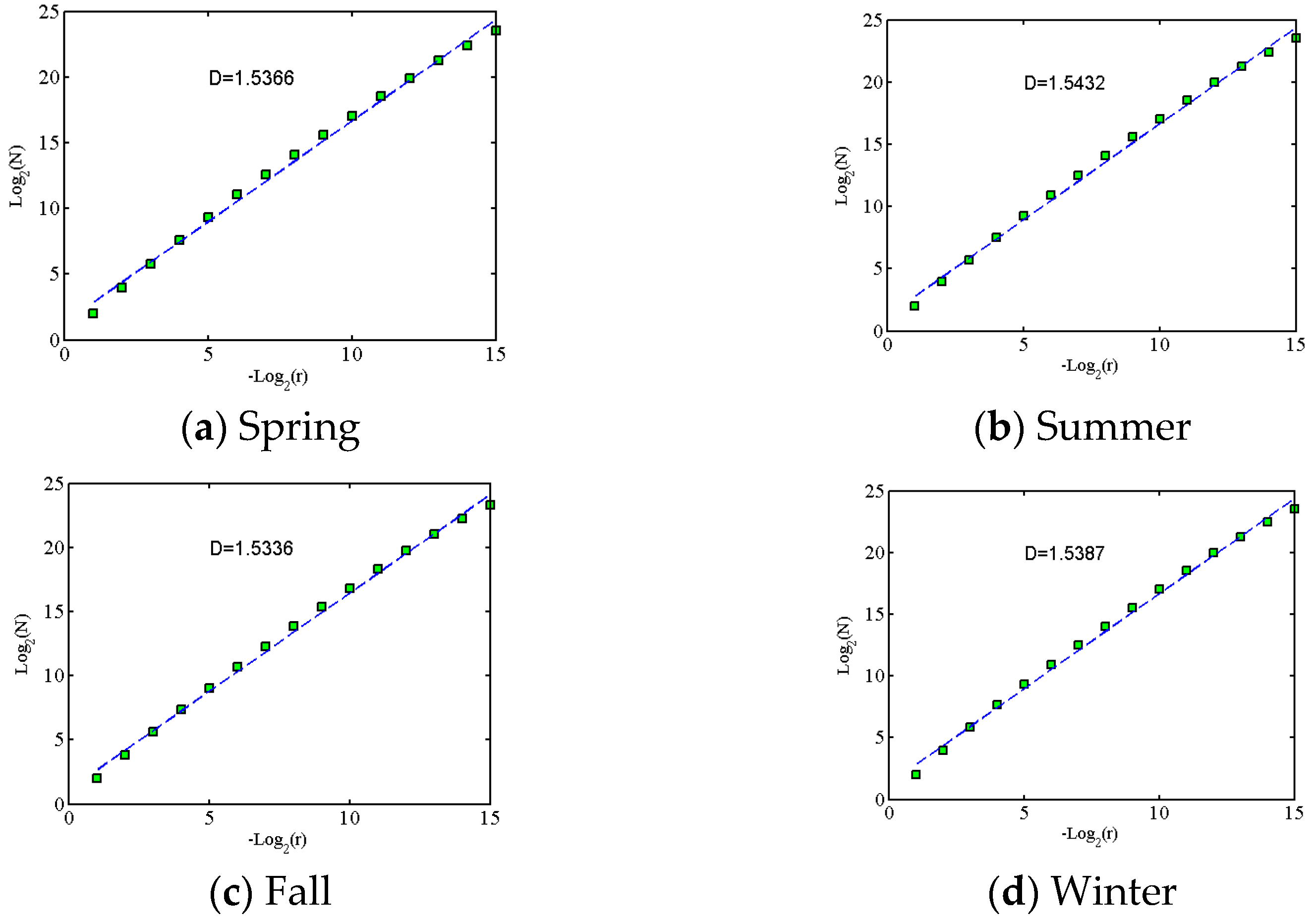
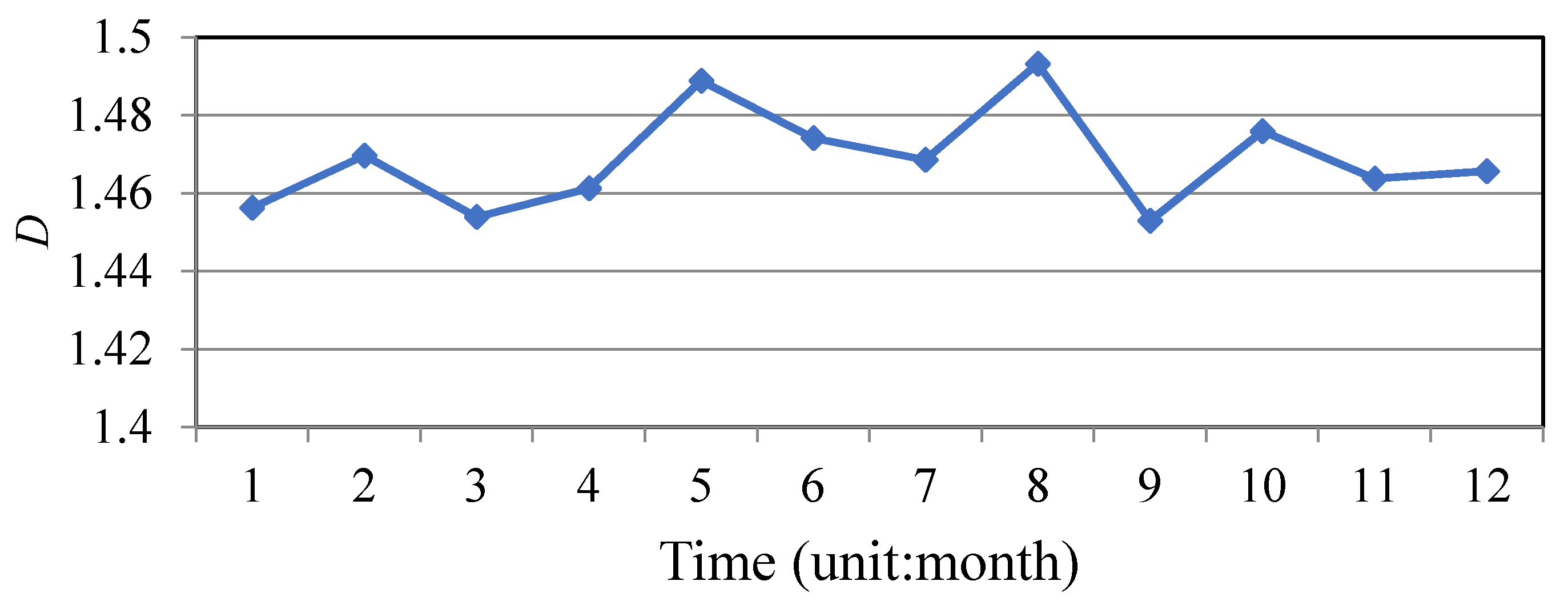
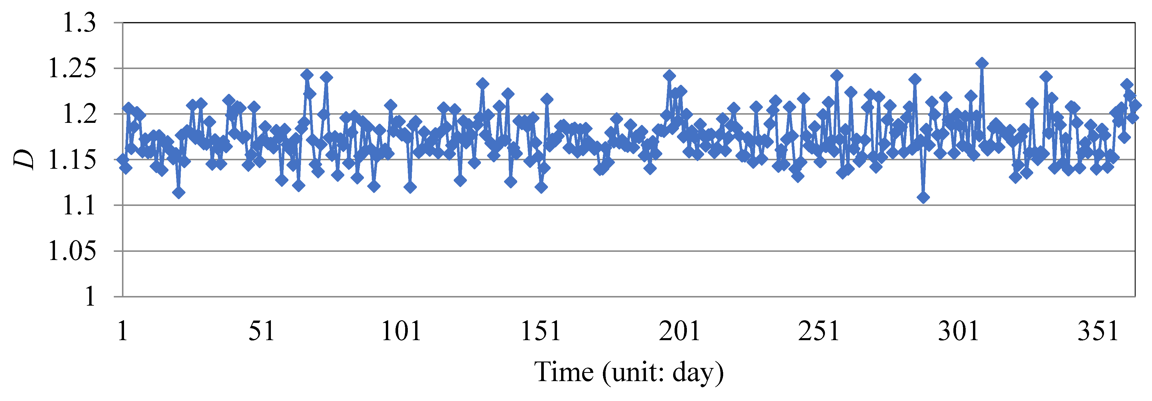
The wind speed data are from Pingtan County, which is located in Fujian Province in the southeastern coastal area of China, where numerous wind farms have been built due to its abundant wind resources. The wind speed data applied in this research are from Yutou Island located in northwestern Pingtan County at a latitude of 25°37′56″ N and longitude of 119°34′45″ E, as shown in Figure 1. The wind speed data are obtained by a field measurement system with three sonic anemometers installed at 10 m, 80 m, and 100 m heights, and six vane anemometers installed at 10 m, 30 m, 50 m, 80 m, 90 m, and 100 m heights. Long-term high-frequency (10 Hz) and low-frequency (1 Hz) data were acquired by field measurements. The 10-min average wind speed data are subjected to chaotic analysis and prediction in the following sections.

3. Fractal Analysis

For wind speed forecasting, the predictability of wind speed mainly depends on persistence, which is dependent on past features. The persistence of wind time speed indicates that the variation in wind speed is somewhat monotonous; therefore, similar wind characteristics can be predicted. Therefore, in this research, the persistence of the described wind speed data is first investigated before the prediction analysis. The concept of fractal dimensional analysis based on chaos theory has been proven to be an efficient way to quantitatively determine the persistence of wind speed. It was first introduced to characterize the complexities of geometry. Discrete time series describes the self-similarity of the series. The fractal dimension of the long-term wind speed data D ranges from 1 to 2. When the value D is between 1 and 1.5, it indicates that the wind speeds have persistence; when it is between 1.5 and 2, the wind speed has anti-persistence, which has low serial correlation in the time domain. As D approaches 1, the wind speed shows increasing persistence. However, when D is approximated to be 1.5, the wind speed is considered a random walk [28]. In this research, the fractal dimension of wind speed at the considered location is calculated by the box counting method [29]. The box counting method has been proven to be an efficient method to estimate the fractal dimension of a picture considering the width of box r and the number of boxes N by the following expression:

$$D={\lim }_{r\to 0}\frac{\log N(r)}{\log (1/r)}$$

(1)

where N(r) is the number of small square grids with width r that need to cover the entire time series.

Figure 2 shows the calculated fractal dimension based on the measured seasonal wind speed data. For the four seasons, fractal dimensions, D, are all approximately 1.5, showing the random walk for seasonal wind speed data. A similar phenomenon can be found in Figure 3, which represents the fractal dimensions for monthly wind speed data. The fractal dimensions for monthly wind speed data are lower than those for seasonal data but also approach 1.5, representing an independent process with less persistence.

Figure 4 illustrates the estimated fractal dimensions for daily wind speed data. The figure shows that the daily fractal dimensions over one year are between 1 and 1.5, which indicates persistence for wind speed data and therefore can be predicted. In the following sections, the 10 min average daily wind speed data are applied to conduct the chaotic analysis and wind speed prediction process.

4. Data Analysis Methods Applied

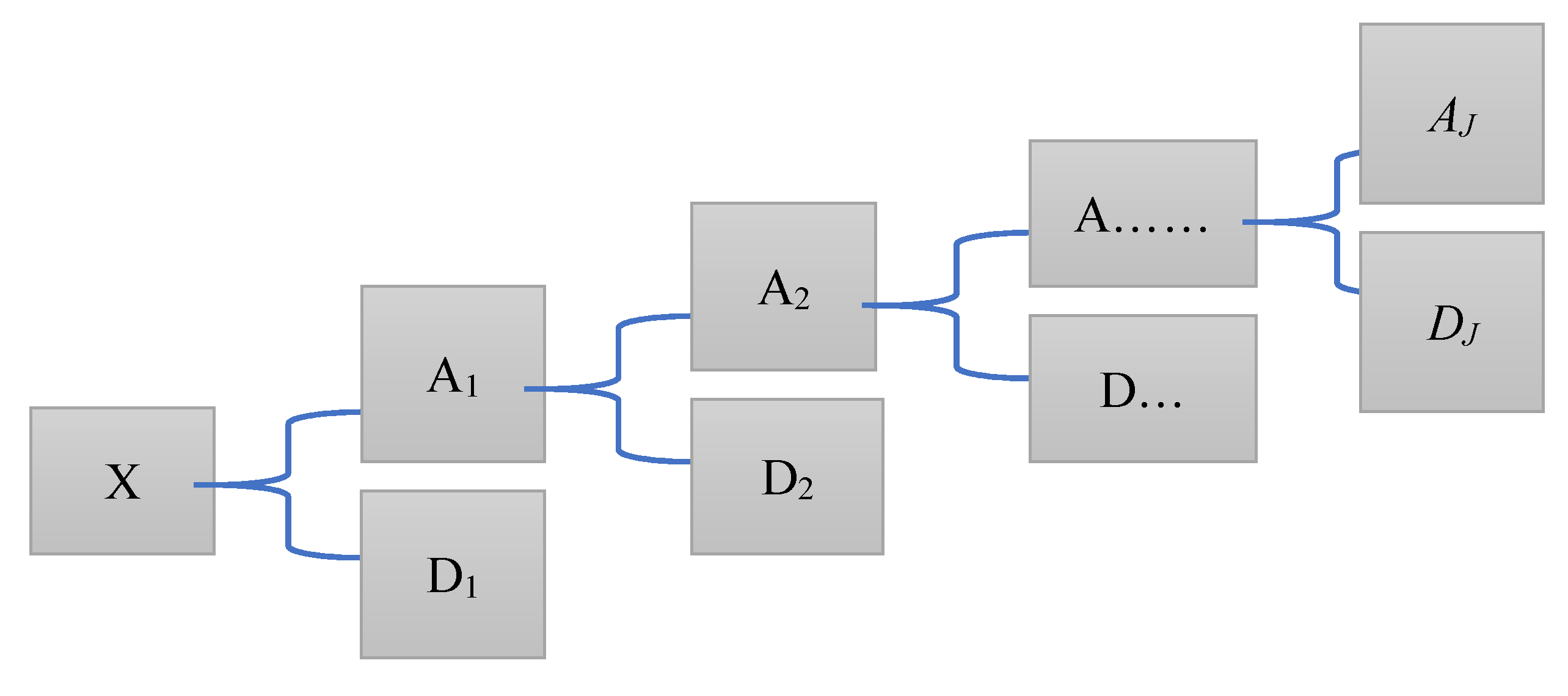
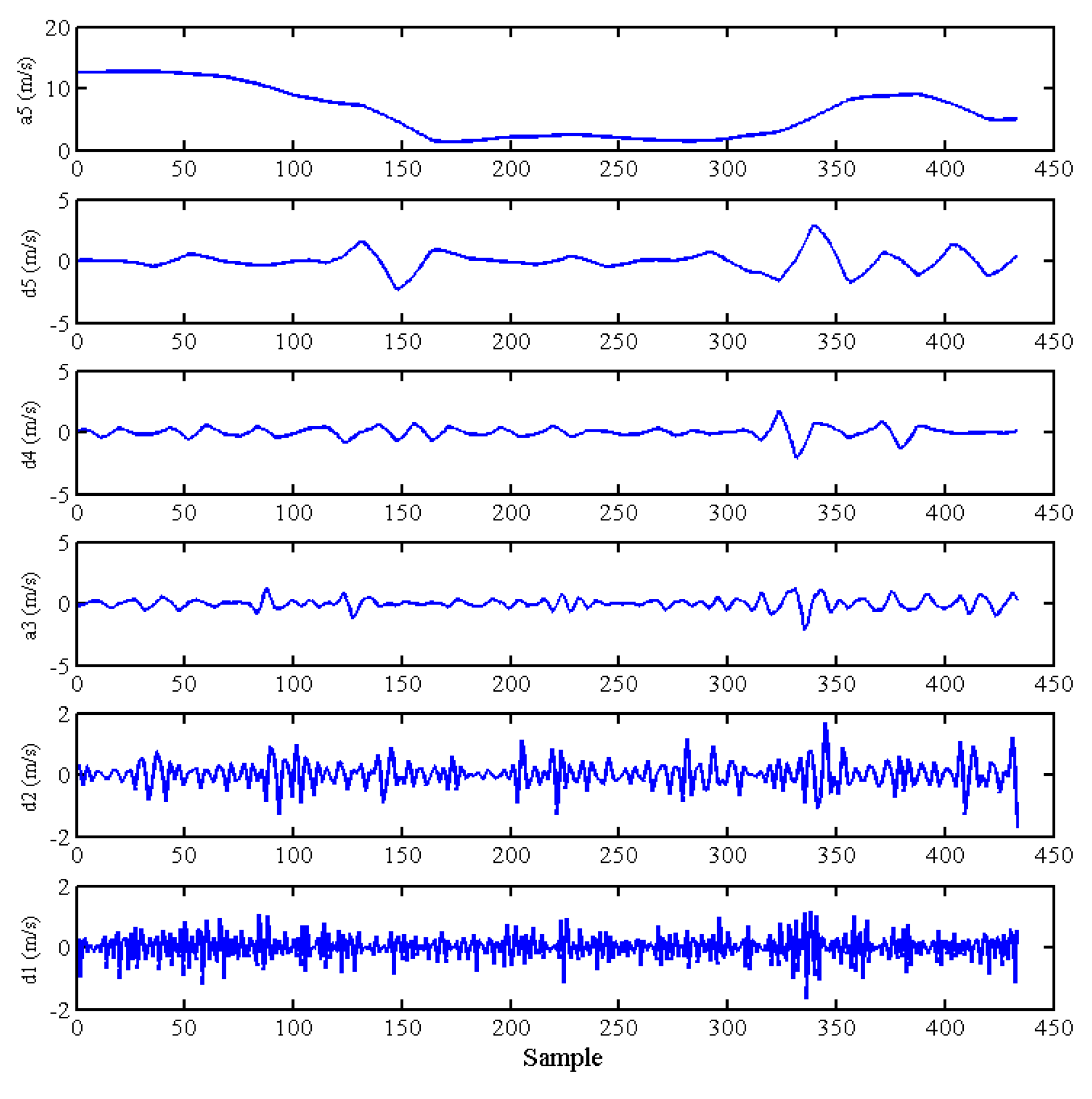
4.1. Wavelet Analysis

Wavelet transformation is a useful method to convert a series of data from the time domain into a representation involving different layers of frequency levels. The original data can be transformed into different frequency components that can be analyzed at a resolution matched to their frequency. Wavelets are localized at both time and scale and can be generated by scaling and translating a single base wavelet called the “mother wavelet”. The lower scale components give finer microscopic details of data at higher resolutions, and the higher scales yield grosser features at lower resolutions [30]. Wavelets are most suited for the study of data, such as those of wind speed, which is inherently multiscale due to contributions from numerous atmospheric and topographic factors. Wavelet transforms are mainly divided into two groups: continuous wavelet transforms (CWTs) and discrete wavelet transforms (DWTs). The CWT can be expressed as [31]:

$${\mathrm{CWT}}_x(a,b)=a^{-0.5}{\displaystyle {\int }_{-\infty }^{\infty }\psi {(t)}^{*}x(t)}dx,a>0$$

(2)

$${\psi }_{a,b}(t)=a^{-0.5}\psi (\frac{t-b}{a}),$$

(3)

where x(t) is the signal to be analyzed, ${\psi }_{a,b}(t)$ is the mother wavelet scaled by a factor a and shifted by a translated parameter b, and * represents the complex conjugate. The discrete wavelet transform can be expressed as:

$${\mathrm{DWT}}_{a,b}={\displaystyle \sum _a{\displaystyle \sum _{b}f(b){\psi }_{n,m}}}$$

(4)

where f refers to the original wind speed time series. With the application of wavelet decomposition, the wind speed time series can be decomposed into a high frequency level and a lower frequency level. The original wind speed data can be expressed as a sum of smoother components and a set of components providing details of the data at high resolutions with the expression:

$$X={\displaystyle \sum _{j=1}^J{D}_j}+A_J$$

(5)

where j represents the decomposed level and A and D represent low frequency and high frequency, respectively. Figure 5 shows the tree structure of the wavelet decomposition.

As discussed in the previous section, the daily wind speed data are proven to have persistence and therefore can be predicted. In this section, the daily 10 min average wind speed data are applied to show wavelet decomposition. Figure 6 shows a decomposition example of wind speed data at five levels. For the decomposed components d1–d5, the frequency bands range from high to low. For higher levels with lower frequencies, the time series shows a smoother tendency, which may have a greater chance of being predicted. In the following section, to fully study the characteristics, the wind time speed data are decomposed at 10 levels. The characteristics of each component are studied, and proper prediction methods are selected to obtain accurate prediction results.

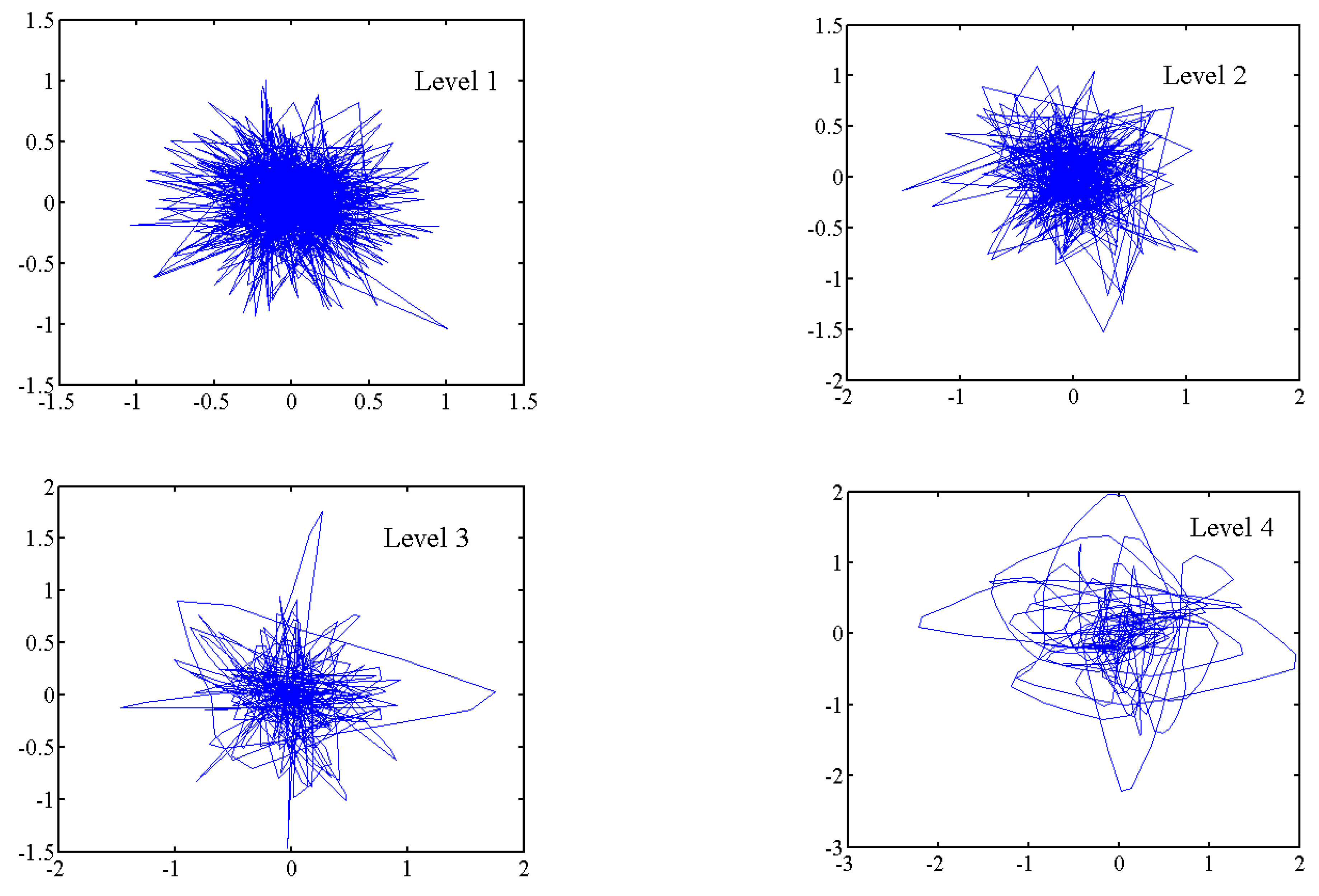
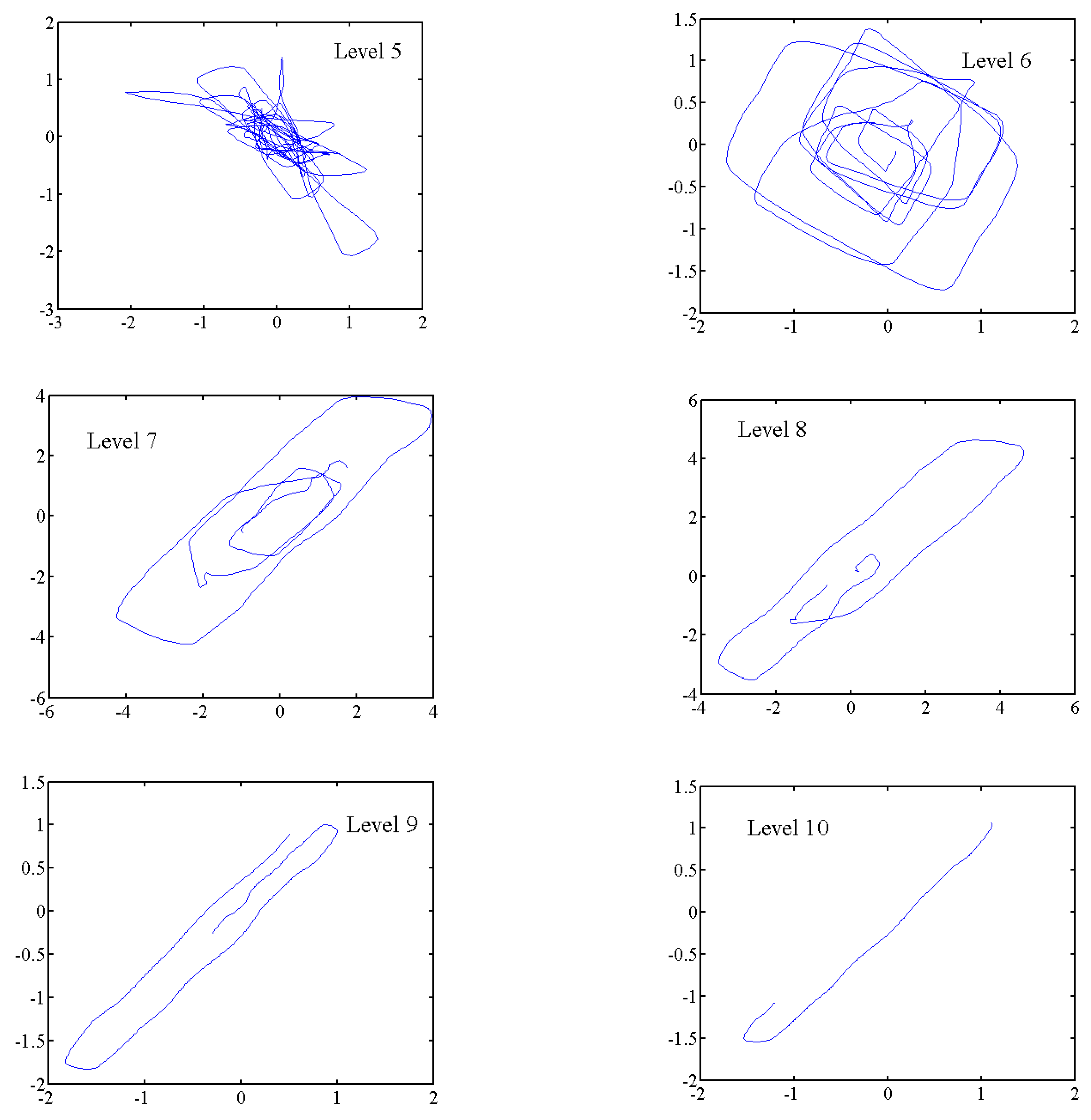
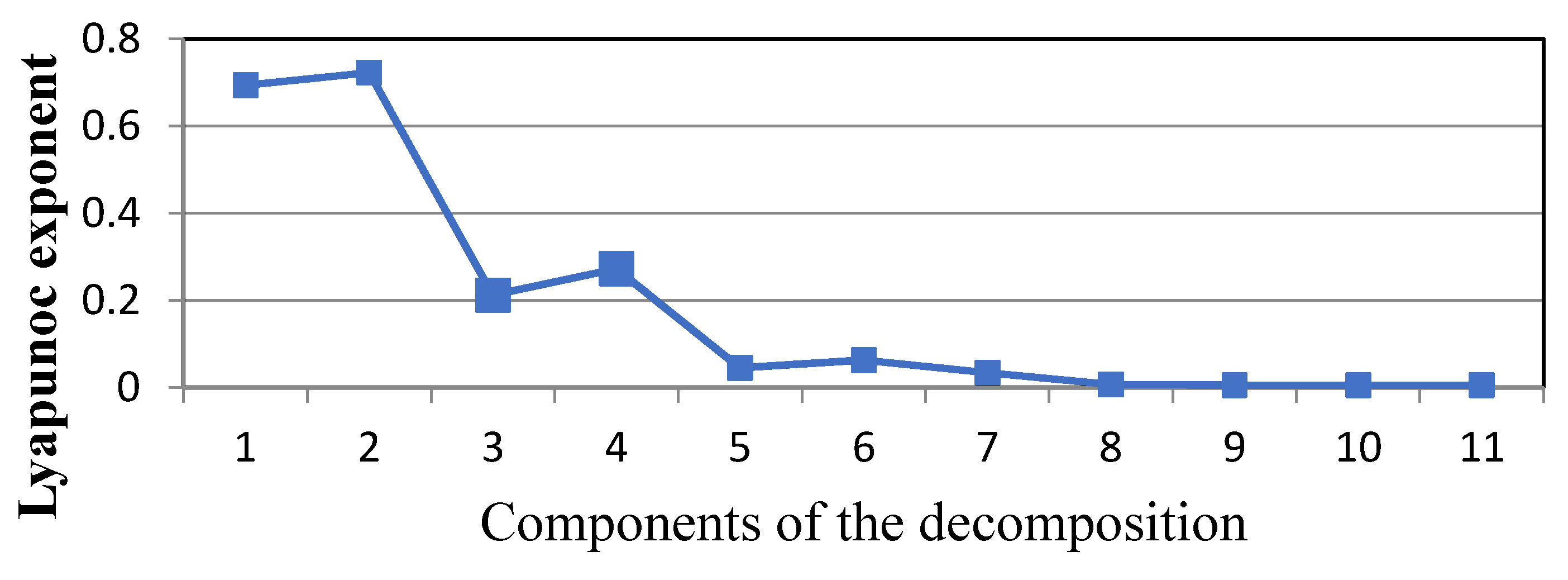
4.2. Chaotic Analysis of the Decomposed Components

One of the important characteristics of chaotic time series is that it is very sensitive to the initial conditions, indicating that the trajectories diverge exponentially. Numerous methods have been developed to diagnose chaotic behaviors for continuous systems, such as the largest Lyapunov exponents [3] and relative specific volume [31]. For a continuous nonlinear system, the largest Lyapunov exponent can be calculated by the definition method to measure the geometric average of the two diverged trajectories. The positive Lyapunov exponent indicates a strong attractor of the system.

The Kanta algorithm [3,32] has been proven to be an efficient method to estimate the largest Lyapunov exponent for a discrete time series with the following expression:

$$S(\Delta n)=\frac{1}{N}{\displaystyle \sum _{N_0=1}^N\ln (\frac{1}{\left|U(y_{N_0})\right|}}{\displaystyle \sum _{\begin{array}{l}i=1,\dots N\\ y_i\in U(y_{N_0})\end{array}}\left|y_{N_0+\Delta n}-y_{N+\Delta n}\right|}$$

(6)

$$y(t)=x(t),x(t-\tau ),x(t-2\tau ),\dots x(t-(m-1)\tau )$$

(7)

where y is the delay vector for the time series, $y_{n_0}$ is a fixed point in the embedding space, and y_n are the points in a neighborhood U(y_n0) of y_n0. When plotting S against the number of iterations n yields a curve with a linear increase, the slope of the curve is the calculated maximum Lyapunov exponent. m and $\tau$ are the embedded dimension and delay time, respectively, which play a significant role in calculating the Lyapunov exponent.

Figure 7 shows the delay representation of the considered system for wavelet components 1–10 with the proper selection of embedding parameters and delay time. As seen in the figure, for the low levels, which represent the high-frequency band, the dynamics of the component are complex. As the level increases, the complexities of dynamics decrease progressively. The dynamics tend to be nearly periodic toward a higher level 10 and lower frequency.

Figure 8 shows the calculated largest Laypunov exponent. The results show a progressive variation in the Lyapunov exponent for each component of the decomposition. For levels 1–7, the time series shows a positive Lyapunov exponent, indicating chaotic characteristics, while for levels 8–11, the Lyapunov exponents are equal to 0, representing a nonchaotic time series.

Another method that is well-accepted to detect chaos is called the Kolmogrov entropy method. Consider a dynamical system with m degrees of freedom, and suppose the F-dimensional phase space to be partitioned to boxes of size ${ϵ}^F$. Suppose there is an attractor in phase space and that the trajectory $\overrightarrow{X}\left(t\right)$ is in the basin of attraction. The calculation of the K entropy can be described as [33]:

$$\mathrm{K}=-\underset{\tau \to 0}{\lim }\underset{r\to 0}{\lim }\underset{m\to \infty }{\lim }1/\left(m\tau \right)\times {\displaystyle \sum }_{i_0\dots i_m}\mathrm{P}\left(i_0,i_1\dots ,i_m\right)\mathrm{lnP}\left(i_0,i_1\dots ,i_m\right)$$

(8)

in which the $\mathrm{P}\left(i_0,i_1\dots ,i_m\right)$ indicate the joint probability that $\overrightarrow{X}\left(t=\tau \right)$ is in box $i_1$, $\overrightarrow{X}\left(t=2\tau \right)$ is in box $i_2$… and $\overrightarrow{X}\left(t=m\tau \right)$ is in the box $i_m$. When K = 0, it indicates an ordered system; K is infinite for a random system, and if K is a non-zero constant, it indicates a chaotic system, and the larger the value, the more chaotic the system is.

Figure 9 shows a calculated K value for each component. As indicated in the figure, the K value is approaching 0 at about 8–11 components. For the components 1–7, the values are all positive, and at the lower levels, the K values are larger, indicating more chaotic time series. This shows agreement with the results of largest Lyapunov exponent.

5. Wind Speed Prediction

5.1. Wind Prediction for Non-Chaotic Components

The Kalman filter (KF) has been proven to be a very efficient mathematical tool that utilizes the feedback control approach to estimate the state of a system [34]. The state of the system is estimated at each interval, and the measurement of the state corrects the estimated state to obtain the measurement feedback. The procedure includes a prediction step and an updating step, which can be expressed as follows. The prior state at step k + 1 estimated from the kth step can be described as:

$${\widehat{x}}_{k+1}^{-}=A{\widehat{x}}_k^{-}+B{u}_k+w_k$$

(9)

where ${\widehat{x}}_k^{-}$ is the state of the system in the kth step, A is the state matrix from k to k + 1, u_k is the input and B represents the input matrix. Therefore, the estimated error covariance at the k + 1 step can be computed as

$$P_{k+1}^{-}=A{P}_k{A}^T+Q$$

(10)

where P_k indicates the error covariance and Q is the process noise covariance. The Kalman gain K is computed as follows by the estimated error covariance and measurement matrix H and measurement noise:

$$K_{k+1}=P_{k+1}^{-}{H}_{k+1}^T{(H_{k+1}{P}_{k+1}^{-}{H}_{k+1}^T+R)}^{-1}$$

(11)

The Kalman gain is applied to update the state and error covariance at the kth step to enhance the estimation accuracy as:

$${\widehat{x}}_{k+1}={\widehat{x}}_{k+1}^{-}+K_{k+1}(z_{k+1}-H_{k+1}{\widehat{x}}_{k+1}^{-});P_{k+1}=(I-K_{k+1}{H}_{k+1})P_{k+1}^{-}$$

(12)

In this research, the Kalman filter is applied to predict discrete wind speed data; therefore, no input is considered; that is, in the calculation, B and u_k are set to 0.

The obtained wind speed data are applied to conduct the prediction. To measure the prediction accuracy, the evaluation criteria are set as the mean relative error (MAPE), mean absolute error (MAE) and root mean square error (RMSE), and the criteria can be defined as:

$$\begin{array}{l}\mathrm{MAPE}=\frac{1}{N}{\displaystyle \sum _{i=1}^N\frac{\left|p(i)-r(i)\right|}{r(i)}}\times 100\%\\ \mathrm{MAE}=\frac{1}{N}{\displaystyle \sum _{i=1}^N\left|p(i)-r(i)\right|}\\ \mathrm{RMSE}=\sqrt{\frac{1}{N}{{\displaystyle \sum _{i=1}^N(p(i)-r(i))}}^2}\end{array}$$

(13)

Here, r(i) is the real wind speed, p(i) is the predicted wind speed, and N is the test sample number for the prediction model. The units for MAPE are nondimensional and are m/s for MAE and RMSE. With the application of the Kalman filter, the prediction of wind speed wavelet decomposition components is conducted. Figure 10 shows the predicted results directly using the Kalman filter method (DKF) for level 1, level 5 and level 10. The RMSE in Figure 11 and MAPE in Figure 12 indicate that level 1–level 7, which have chaotic characteristics, are not suitable for the Kalman filter prediction method with the corresponding large RMSE and MAPE values. Therefore, the chaotic prediction method for positive Lyapunov exponent levels is applied in this paper.

5.2. Wind Prediction for Chaotic Components

In this research, adaptive Volterra prediction, which has been widely used for chaotic prediction, is applied to conduct prediction for chaotic time series by using the Volterra series approximation [35]. The main concept can be described as follows. For a time series, $X(n)=x(n),x(n-\tau ),\dots x(n-(m-1)\tau )$, the one-step prediction can be expressed by the Volterra approximation:

$$\widehat{x}(n+1)=h_0+{\displaystyle \sum _{k=1}^p{y}_k(n)};y_k(n)={\displaystyle \sum _{m_1,m_2\dots m_k}^{m-1}{h}_k(m_1,m_2},\dots m_k){\displaystyle \prod _{i=1}^{k}x(n-m_i}\tau )$$

(14)

$h_k(m_1,m_2,\dots m_k)$ is the kth Volterra core, and p is the order of the Volterra filter. Taking m as 2, the one-step prediction can be rewritten as:

$$\widehat{x}(n+1)=H^T(n)U(n)$$

(15)

in which,

$$U(n)=[1,x(n),x(n-\tau ),\dots x(n-(m-1)\tau ),x^2(n),x(n)x(n-\tau )\dots x^2(n-(m-1)\tau )]$$

(16)

$$H(n)={[h_0,h_1(0),h(1),\dots ,h(m-1),h_2(0,0),h_2(0,1),\dots ,h_2(m-1,m-1)]}^T$$

(17)

The coefficient vector can be determined by the time domain orthogonal method.

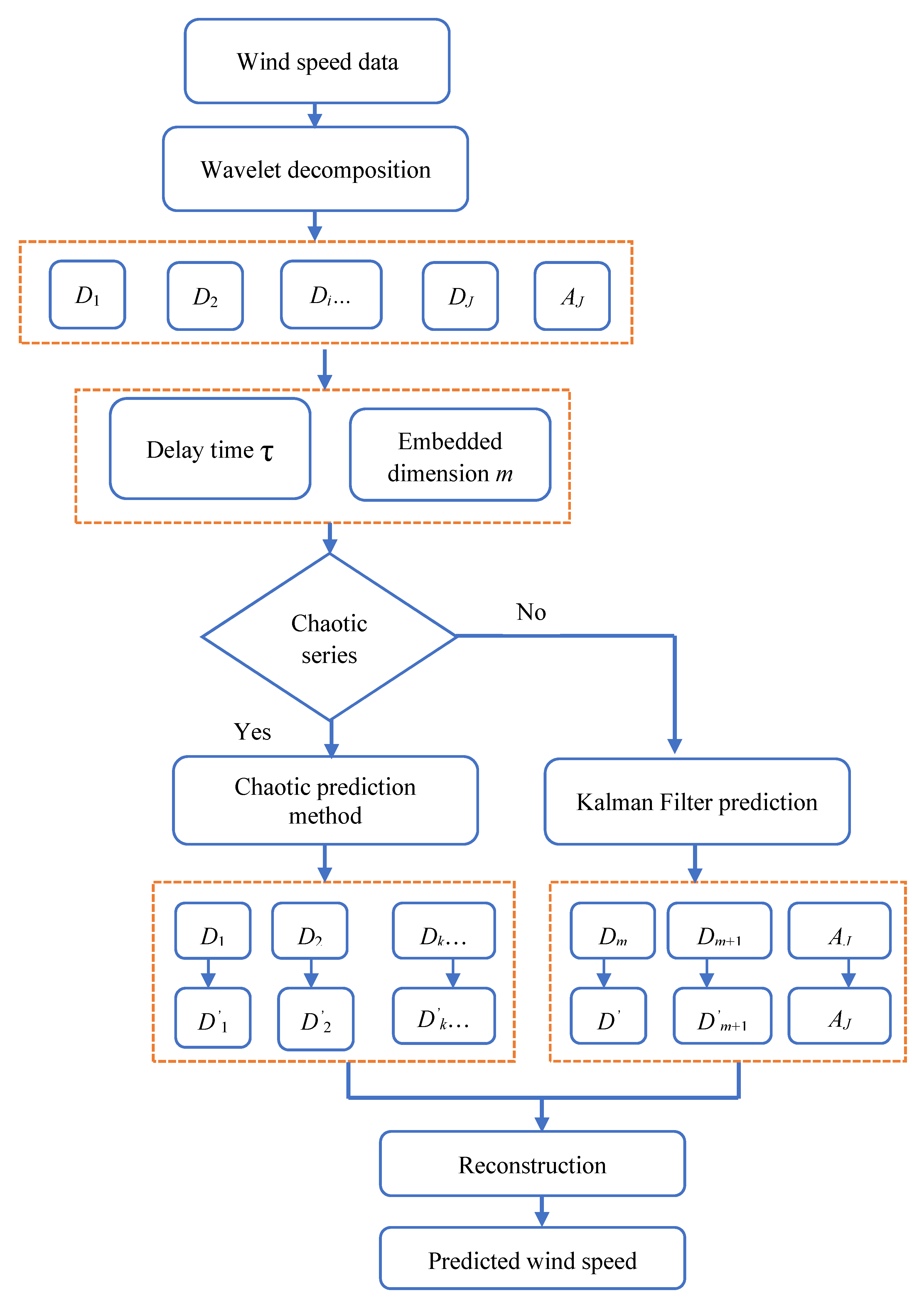
5.3. A Hybrid Prediction Method Combining Wavelet Decomposition

With the application of the Volterra filter and Kalman filter, a new hybrid method to predict wind speed can be proposed in this research. The wind speed data are first decomposed using wavelet decomposition, and high-frequency and low-frequency bands are consequently separated. Chaotic characteristics are then found using the largest Lyapunov exponents. Then, chaotic components are predicted by using the Volterra filter, which has been widely used for chaotic time series prediction, and non-chaotic components are predicted by using the Kalman filter. Finally, the predicted components are reconstructed to obtain the predicted wind speed. Criteria such as MAPE, MAE and RMSE are applied to calculate the predicted results. A comprehensive flow chart of the proposed prediction method for wind speed time series can be found in Figure 13.

To make the concept of the proposed method more clear, a comprehensive review for the previous sections may be needed. The wind speed prediction in this research is based on the wind speed data recorded by wind field measurements; therefore, the description of wind speed data is presented in Section 2. Then in Section 3, the fractal dimensions of recorded wind speed data are calculated at different time scales (month and day). Results show the fractal dimension for daily wind speed is around 1.3, indicating it has persistence and daily data would be applied for wind prediction. Section 4 introduces data analysis methods: the wavelet decomposition method and chaotic diagnosis method. Section 5 introduces two prediction methods: Kalman filter to predict non-chaotic components method and the Volterra prediction method to predict chaotic components. The predictions by Kalman filter for each component are conducted, and results show that the Kalman filter can only accurately predict the low-frequency components. Therefore, a hybrid method is introduced with the process: the wind speed data is first decomposed by wavelet decomposition; chaotic analysis is applied to diagnose the components; the Volterra prediction method is applied to predict the chaotic components; the Kalman filter is applied to predict the non-chaotic components; then, the predicted components are combined to obtain the final predicted results.

6. Results and Discussion

The analysis of predictions using KF with and without wavelet decomposition is presented for predictions at different time scales in the following sections. Taking 10-min average wind speed data as samples, Figure 14 shows the comparison of 24-h wind speed prediction results on Yutou Island using the direct Kalman filter (DK), wavelet decomposition and Kalman filter method (WD + KF) and the proposed hybrid method. Forecast errors measured from absolute relative error and mean absolute relative errors are presented in Figure 15. The MAPEs of DKF and WD + DKF were 8.12% and 8.15%, respectively, which was close, indicating that wavelet decomposition could hardly improve the prediction accuracy by using only the Kalman filter. However, with the application of the chaotic prediction method, the MAPE was reduced to 2.62%, indicating that the proposed method could significantly enhance the forecast accuracy of the daily wind speed. This conclusion can also be found in

Table 1. Forecast results of the three methods.

Prediction Method	MAPE (%)	RMSE (m/s)	MAE (m/s)
DKF	8.30	0.70	0.56
WD+KF	8.15	0.65	0.46
Proposed	2.62	0.23	0.18

, which shows the forecast results for the three considered models measured by using three criteria. Similarly to MAPE, with the application of wavelet decomposition, the prediction could be improved compared to the direct Kalman filter method; however, the effect was limited. Using the proposed method, the forecast reliability could be improved by approximately 67.8%, which is very significant in wind industry areas.

In Figure 16, the relative errors from different prediction methods via wind speed are presented. Analogous to Figure 14, improved prediction accuracy could still be found using the proposed method. However, another significant conclusion could be clearly seen: the relative errors showed a decreasing tendency with increasing wind speed. That is, it had more difficulty predicting lower wind speeds. Figure 17 shows the probability density and cumulative probability of the prediction error using the proposed method, and the fitted result based on a normal distribution indicated that the prediction results were reliable such that the error was mostly random.

Figure 18 shows two days ahead wind speed prediction results based on the different methods. The proposed method had the smallest relative error of the three compared methods. The MAPEs for DKF, WD + KF, and the proposed method were 7.62%, 7.76% and 3.49% respectively. Comparing with the MAPE for one day and two days ahead prediction, the two days prediction showed a larger MAPE. This indicates that for the longer time interval, the proposed method showed less accuracy; however, comparing the three methods, the proposed method showed the best prediction performance.

In the previous simulation and discussion, the wind speed data were decomposed at 10 levels. To comprehensively study the influence of wavelet decomposition on the prediction results, different predictions were conducted using wavelet decomposition at 3–12 levels, and the corresponding results are presented in Figure 19. A progressively decreasing tendency with increasing levels can be seen in Figure 19. From level 3–level 7, the errors could be reduced at a significant value; however, after level 7, the level of wavelet decomposition had a limited effect on the wind speed forecast results, indicating that for the considered wind speed data, decomposing the time series was sufficiently accurate to conduct the prediction.

In previous investigations, the analysis was a 24-h prediction based on 10-min average wind speed data. However, other factors, such as the considered time scales and prediction length, may also affect the final results. Figure 20 shows the one-day ahead prediction results based on the obtained hourly data. Analogously, the proposed method showed better performance than the DKF and WD+KF methods, with almost all relative errors within 10%. Moreover, the calculated RMSE for prediction using hourly data was 0.29 m/s. When predicting hourly data based on 10-min average data, the RMSE was 0.16 m/s, which was less than that predicted using hourly data.

7. Conclusions

The analysis of wind speed data has been increasingly essential in wind engineering due to its significance in wind-induced vibration, the design of structures and wind power industry areas. In this research, long-term wind speed data measured in Pingtan, China, were considered subject to persistence analysis, chaotic analysis and prediction. Some meaningful results were obtained.

• With the application of fractal dimensional analysis, the seasonal and monthly wind speed data were considered random with fractal dimensions of approximately 1.5. The daily wind speed data were proven to have persistence and could be predicted with fractal dimensions between 1.1 and 1.3.
• To study the wind speed at a frequency level, the wavelet decomposition method was applied to separate the wind speed data from components at different frequency levels. Chaotic behaviors were found at high frequency levels.
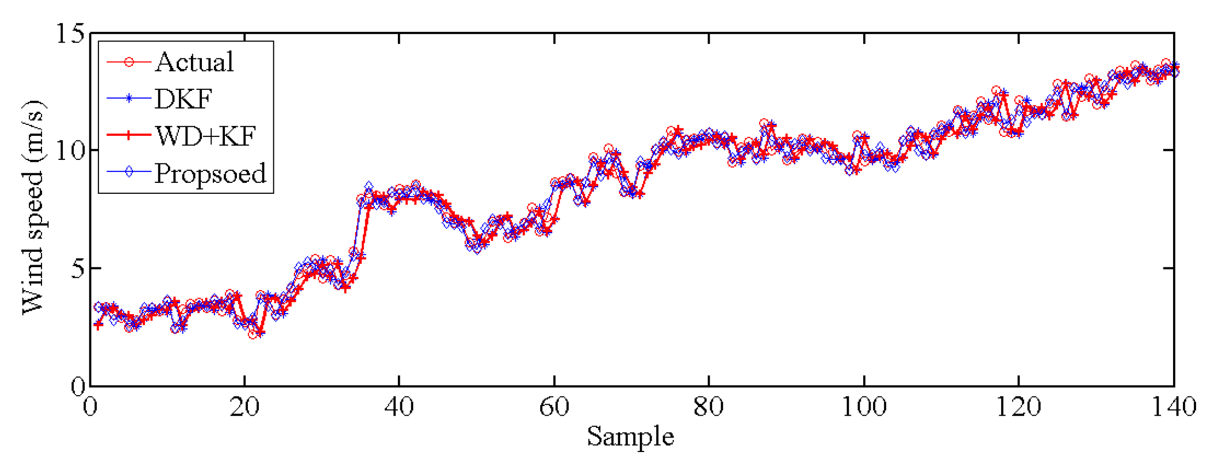
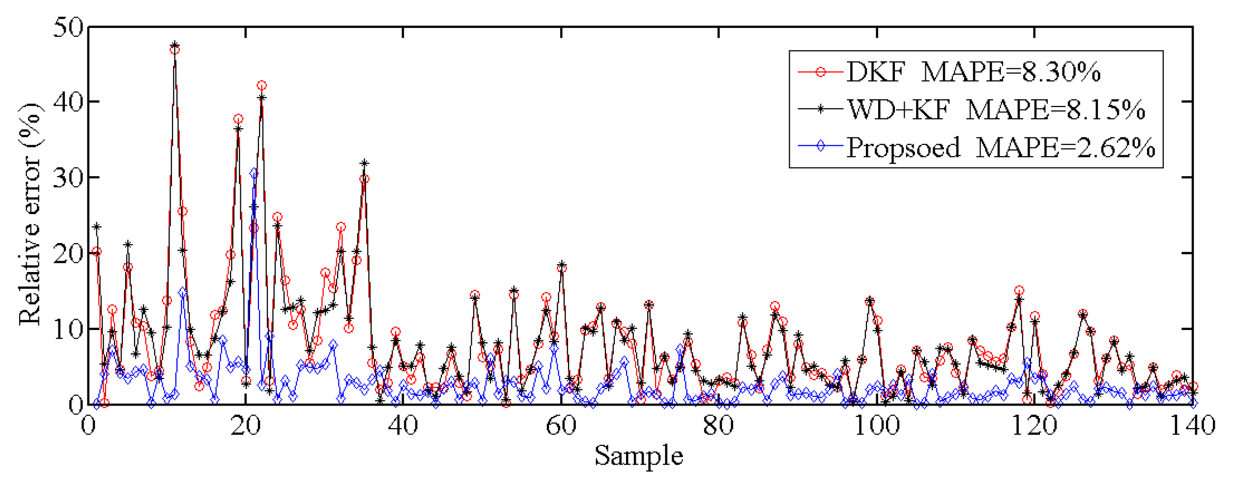
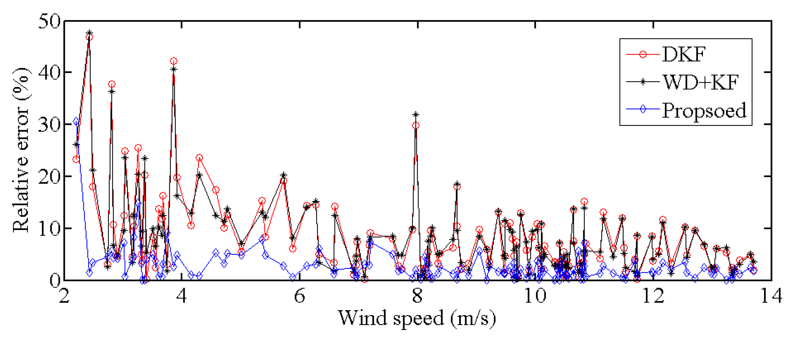
• With the application of the Kalman filter and Volterra prediction method, the wind speed could be accurately predicted with an improvement of 67.8% compared to other prediction methods.
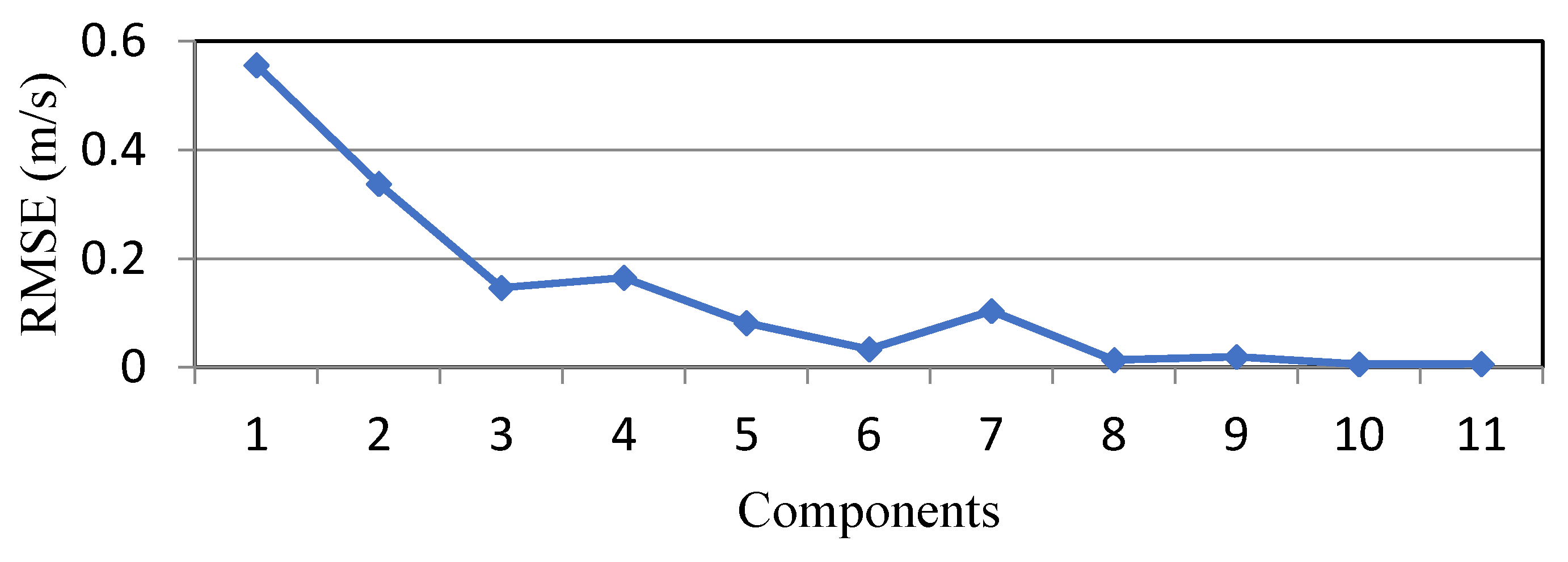
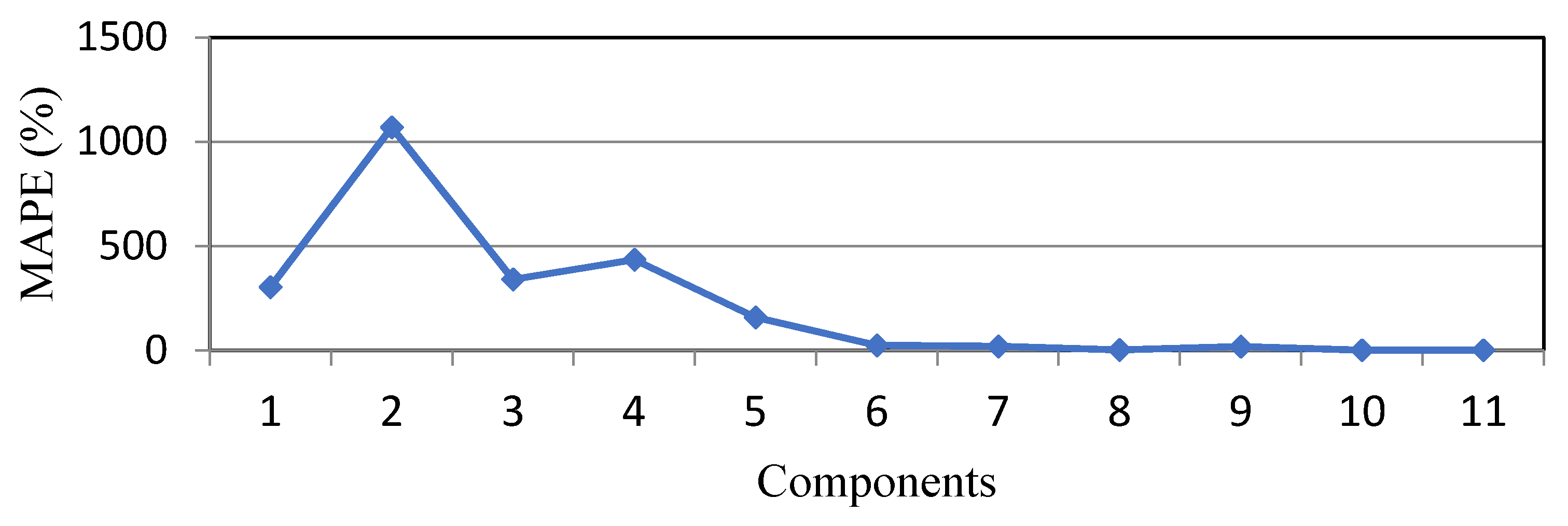
• For the proposed prediction method, the decomposition levels may affect the predictions. The results showed that with a higher decomposition level, the forecasting level is improved; however, for the considered wind speed, the forecast error changed little after level 7.
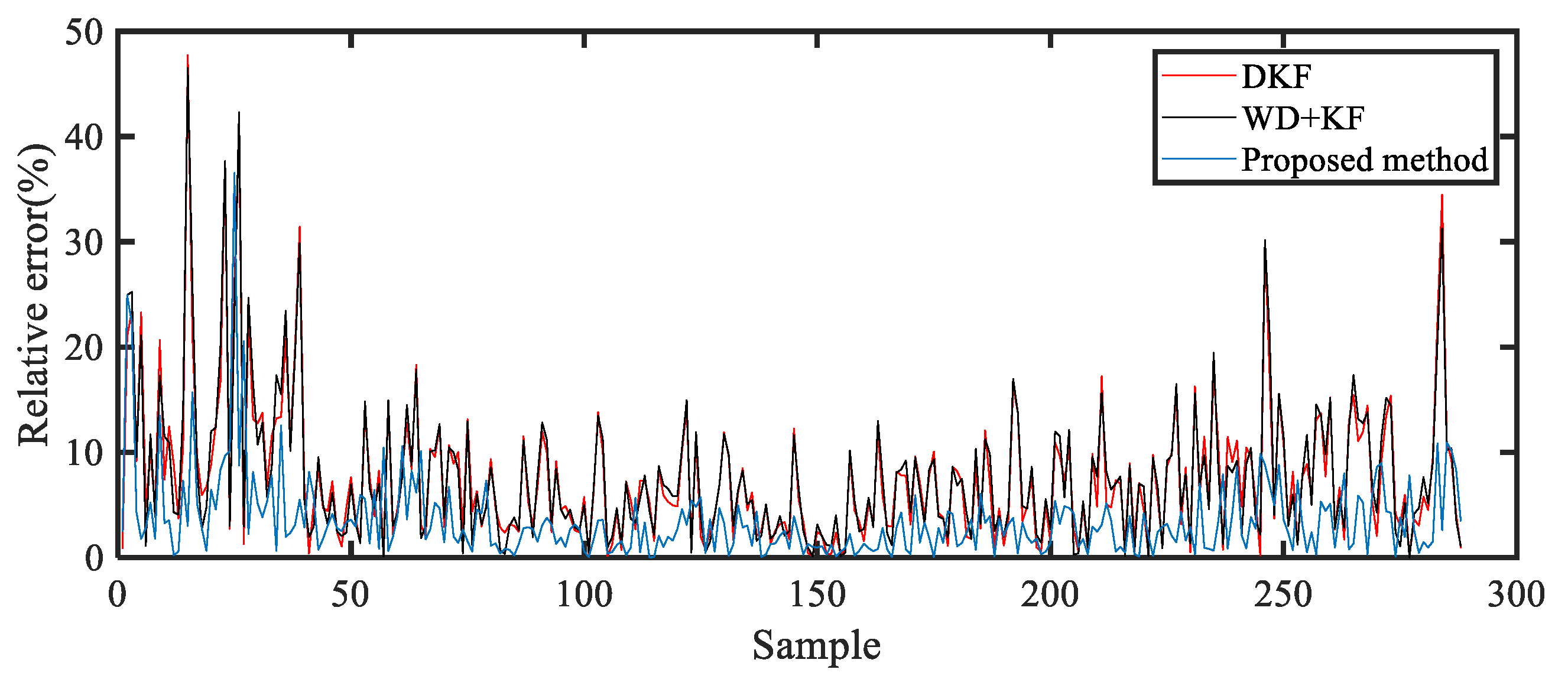
• Moreover, the proposed method showed better performance forecasting hourly data than the 10-min data.

References

1. Tu, Q.; Betz, R.; Mo, J.L.; Fan, Y.; Liu, Y. Achieving grid parity of wind power in China-Present levelized cost of electricity and future evolution. Appl. Energy 2019, 250, 1053–1064. [Google Scholar] [CrossRef]
2. Wang, S.; Li, B.; Li, G.; Yao, B.; Wu, J. Short-term wind power prediction based on multidimensional data cleaning and feature reconfiguration. Appl. Energy 2021, 292, 116851. [Google Scholar] [CrossRef]
3. Drisya, G.; Asokan, K.; Kumar, K.S. Diverse dynamical characteristics across the frequency spectrum of wind speed fluctuations. Renew. Energy 2018, 119, 540–550. [Google Scholar]
4. Wang, X.; Hui, L. Multiscale prediction of wind speed and output power for the wind farm. J. Control Theory Appl. 2012, 10, 251–258. [Google Scholar] [CrossRef]
5. Cadenas, E.; Campos-Amezcua, R.; Rivera, W.; Espinosa-Medina, M.A.; Méndez-Gordillo, A.R.; Rangel, E.; Tena, J. Wind speed variability study based on the Hurst coefficient and fractal dimensional analysis. Energy Sci. Eng. 2019, 7, 361–378. [Google Scholar] [CrossRef]
6. Chang, T.-P.; Ko, H.-H.; Liu, F.-J.; Chen, P.-H.; Chang, Y.-P.; Liang, Y.-H.; Jang, H.-Y.; Lin, T.-C.; Chen, Y.-H. Fractal dimension of wind speed time series. Appl. Energy 2012, 93, 742–749. [Google Scholar] [CrossRef]
7. Harrouni, S.; Guessoum, A. Using a fractal dimension to quantify long-range persistence in global solar radiation. Chaos Solut. Fractal 2009, 41, 1520–1530. [Google Scholar] [CrossRef]
8. Telesca, L.; Lovallo, M.; Kanevski, M. Power spectrum and multi-fractal detrended fluctuation analysis of high-frequency wind measurements in mountainous regions. Appl. Energy 2016, 162, 1052–1061. [Google Scholar] [CrossRef]
9. Ouyang, T.; Cha, X.; Qin, L. Medium-or long-term wind power prediction with combined models of meteorological multivariable. Power Syst. Technol. 2016, 40, 847–852. [Google Scholar]
10. Sun, H.; Qiu, C.; Lu, L.; Gao, X.; Chen, J.; Yang, H. Wind turbine power modeling and optimization using artificial neural network with wind field experimental data. Appl. Energy 2020, 280, 115880. [Google Scholar] [CrossRef]
11. Yan, C.; Pan, Y.; Archer, C.L. A general method to estimate wind farm power using artificial neural networks. Wind Energy 2019, 22, 1421–1432. [Google Scholar] [CrossRef]
12. Díaz, S.; Carta, J.A.; Matías, J.M. Comparison of several measure-correlate-predict models using support vector regression techniques to estimate wind power densities. A case study. Energy Convers. Manag. 2017, 140, 362–400. [Google Scholar] [CrossRef]
13. Sheta, A.F.; Ahmed, S.E.M.; Faris, H. A Comparison between regression, artificial neural networks and support vector machines for predicting stock Market Index. Int. J. Adv. Res. Artif. Intell. 2015, 4, 55–63. [Google Scholar]
14. Shirzad, A.; Tabesh, M.; Farmani, R. A comparison between performance of support vector regression and artificial neural network in prediction of pipe burst rate in water distribution networks. KSCE J. Civ. Eng. 2014, 18, 941–948. [Google Scholar] [CrossRef]
15. Zhang, G.P. Time series forecasting using a hybrid ARIMA and neural network model. Neurocomputing 2003, 50, 159–175. [Google Scholar] [CrossRef]
16. Torres, J.L.; García a De Blas, M.; De Francisco, A. Forecast of hourly average wind speed with ARMA models in Navarre (Spain). Sol. Energy 2005, 79, 65–77. [Google Scholar] [CrossRef]
17. Zhang, Z.; Qin, H.; Liu, Y.; Wang, Y.; Yao, L.; Li, Q.; Li, J.; Pei, S. Long short-term memory network based on neighborhood gates for processing complex causality in wind speed prediction. Energy Convers. Manag. 2019, 192, 37–51. [Google Scholar] [CrossRef]
18. Zuluaga, C.D.; Álvarez, M.A.; Giraldo, E. Short-term wind speed prediction based on robust Kalman filtering: An experimental comparison. Appl. Energy 2015, 156, 321–330. [Google Scholar] [CrossRef]
19. Okumus, I.; Dinler, A. Current status of wind energy forecasting and a hybrid method for hourly predictions. Energy Convers. Manag. 2016, 123, 362–371. [Google Scholar] [CrossRef]
20. Tascikaraoglu, A.; Uzunoglu, M. A review of combined approaches for prediction of short-term wind speed and power. Renew. Sustain. Energy Rev. 2014, 34, 243–254. [Google Scholar] [CrossRef]
21. Zhang, W.Y.; Qu, Z.X.; Zhang, K.Q.; Mao, W.Q.; Ma, Y.N.; Fan, X. A combined model based on CEEMDAN and modified flower pollination algorithm for wind speed forecasting. Energy Convers. Manag. 2017, 136, 439–451. [Google Scholar] [CrossRef]
22. Song, J.J.; Wang, J.Z.; Lu, H.Y. A novel combined model based on advanced optimization algorithm for short-term wind speed forecasting. Appl. Energy 2018, 215, 643–658. [Google Scholar] [CrossRef]
23. Chen, J.; Zeng, G.-Q.; Zhou, W.; Du, W.; Lu, K.-D. Wind speed forecasting using nonlinear-learning ensemble of deep learning time series prediction and extremal optimization. Energy Convers. Manag. 2018, 165, 681–695. [Google Scholar] [CrossRef]
24. An, X.; Jiang, D.; Zhao, M.; Liu, C. Short-term prediction of wind power using EMD and chaotic theory. Commun. Nonlinear Sci. Numer. Simulat. 2012, 17, 1036–1042. [Google Scholar] [CrossRef]
25. Kawauchi, S.; Sugihara, H.; Sasaki, H. Development of very-short-term load forecasting based on chaos theory. Electr. Eng. Jpn. 2004, 148, 55–63. [Google Scholar] [CrossRef]
26. Jiang, Y.; Huang, G.; Yang, Q.; Yan, Z.; Zhang, C. A novel probabilistic wind speed prediction approach using real time refined variational model decomposition and conditional kernel density estimation. Energy Convers. Manag. 2019, 185, 758–773. [Google Scholar] [CrossRef]
27. An, X.; Jiang, D.; Liu, C.; Zhao, M. Wind farm power prediction based on wavelet decomposition and chaotic time series. Expert Syst. Appl. 2011, 38, 11280–11285. [Google Scholar] [CrossRef]
28. Harrouni, S. Long term persistence in daily wind speed series using fractal dimension. Int. J. Multiphys. 2016, 7, 87–94. [Google Scholar] [CrossRef] [Green Version]
29. Soille, P.; Rivest, J.F. On the validity of fractal dimension measurements in image analysis. J. Vis. Commun. Image Represent. 1996, 7, 217–229. [Google Scholar] [CrossRef]
30. Daubechies, I. Ten Lectures on Wavelets; SIAM, Society for Industrial and Applied Mathematics: Philadelphia, PA, USA, 1992; Volume 61. [Google Scholar]
31. Tutueva, A.V.; Karimov, T.I. Detection of Hidden Oscillations in system without equilibrium. Int. J. Bifurc. Chaos 2021, 31, 20150043. [Google Scholar] [CrossRef]
32. Kantz, H.; Schreiber, T. Nonlinear Time Series Analysis; Cambridge University Press: Cambridge, UK, 2004; Volume 7. [Google Scholar]
33. Grassberger, P. Estimation of the Kolmogorov entropy from a chaotic signal. Phys. Rev. A 1983, 28, 2591–2593. [Google Scholar] [CrossRef] [Green Version]
34. Julier, S.J.; Uhlmann, J.K.; Durrant-Whyte, H.F. A new approach for filtering nonlinear systems. Proc. Am. Control Conf. 1995, 128, 1628–1632. [Google Scholar]
35. Billings, S.A.; Boaghe, O.M. The Response Spectrum Map, Volterra Series Representations and the Duffing Equation; The Department of Automatic Control & Systems Engineering, The University of Sheffield: Sheffield, UK, 1999. [Google Scholar]
Figure 1. Location of stations on Yutou Island.
Processes 09 01793 g001
Figure 2. Fractal dimension of seasonal wind speed ((a): Spring; (b): Summer; (c): Fall; (d): Winter).
Processes 09 01793 g002
Figure 3. Fractal dimension of monthly wind speed.
Processes 09 01793 g003
Figure 4. Fractal dimension of daily wind speed.
Processes 09 01793 g004
Figure 5. Wavelet decomposition of wind speed.
Processes 09 01793 g005
Figure 6. An example of wind speed decomposition using wavelet decomposition.
Processes 09 01793 g006
Figure 7. Time delay construction ( x n and x n d ) for each component (level 1–level 10) using wavelet decomposition of wind speed time series.
Processes 09 01793 g007aProcesses 09 01793 g007b
Figure 8. Lyapunov exponent of each level.
Processes 09 01793 g008
Figure 9. K entropy values of each level.
Processes 09 01793 g009
Figure 10. Wind speed prediction directly using DKF.
Processes 09 01793 g010
Figure 11. RMSE of prediction for each level using DKF.
Processes 09 01793 g011
Figure 12. MAPE of prediction for each level using DKF.
Processes 09 01793 g012
Figure 13. Flow chart of the prediction.
Processes 09 01793 g013
Figure 14. Prediction results from the different methods.
Processes 09 01793 g014
Figure 15. Prediction errors from the different methods.
Processes 09 01793 g015
Figure 16. Prediction errors via wind speed.
Processes 09 01793 g016
Figure 17. PDF and CDF of the prediction error using the proposed method.
Processes 09 01793 g017
Figure 18. Two days ahead prediction errors based on the different methods.
Processes 09 01793 g018
Figure 19. Prediction results at different decomposition levels.
Processes 09 01793 g019
Figure 20. Prediction errors from the different methods based on hourly data.
Processes 09 01793 g020