Modified Multi-Crossover Operator NSGA-III for Solving Low Carbon Flexible Job Shop Scheduling Problem

Abstract

Low carbon manufacturing has received increasingly more attention in the context of global warming. The flexible job shop scheduling problem (FJSP) widely exists in various manufacturing processes. Researchers have always emphasized manufacturing efficiency and economic benefits while ignoring environmental impacts. In this paper, considering carbon emissions, a multi-objective flexible job shop scheduling problem (MO-FJSP) mathematical model with minimum completion time, carbon emission, and machine load is established. To solve this problem, we study six variants of the non-dominated sorting genetic algorithm-III (NSGA-III). We find that some variants have better search capability in the MO-FJSP decision space. When the solution set is close to the Pareto frontier, the development ability of the NSGA-III variant in the decision space shows a difference. According to the research, we combine Pareto dominance with indicator-based thought. By utilizing three existing crossover operators, a modified NSGA-III (co-evolutionary NSGA-III (NSGA-III-COE) incorporated with the multi-group co-evolution and the natural selection is proposed. By comparing with three NSGA-III variants and five multi-objective evolutionary algorithms (MOEAs) on 27 well-known FJSP benchmark instances, it is found that the NSGA-III-COE greatly improves the speed of convergence and the ability to jump out of local optimum while maintaining the diversity of the population. From the experimental results, it can be concluded that the NSGA-III-COE has significant advantages in solving the low carbon MO-FJSP.

1. Introduction

The flexible job scheduling problem (FJSP) is an extension of the classic job scheduling problem (JSP) and is closer to the actual production environment. In the scheduling process of the FJSP, processing operations can be processed on all optional machines. The assignable machine expands the search range of feasible solutions and also increases the complexity and the difficulty of solving the problem. The FJSP is a complex NP-hard problem, and its solution time increases exponentially as the problem size increases.

With the increasingly prominent energy crisis and environmental pollution, manufacturing has gradually become one of the hot spots in modern manufacturing. Manufacturing has adopted a new sustainable manufacturing model that has attracted widespread attention from industry and academia. In the manufacturing process of an enterprise, workshop scheduling is an important factor in the manufacturing process. It not only affects the production efficiency and the economic benefits of the enterprise but also is closely related to the social responsibility of the enterprise. Therefore, it has important theoretical and practical significance to conducting research on flexible job scheduling with the goal of protecting the environment and saving energy.

In the past few decades, the single-objective FJSP (SO-FJSP), which has been extensively studied in the literature, has usually sought to minimize the total completion time [1,2,3,4,5,6]. However, many realistic scheduling problems often need to optimize multiple objectives at the same time, and these objectives usually conflict with each other. The main method used to solve the MO-FJSP is the MOEA, which can be roughly divided into two categories: the weighting method and the Pareto method. The weighting method solves the MO-FJSP by assigning different weights to each objective and transforming the multi-objective problem into a single-objective problem. The Pareto method solves the MO-FJSP based on the Pareto dominance relationship and generates a set of Pareto optimal solutions. As a Pareto method, the non-dominated sorting genetic algorithm-II (NSGA-II) [7] is an effective method to solve various multi-objective optimization problems in recent years. Z.-Q. Jiang et al. [8] used the NSGA-II algorithm, which optimizes mutation strategies to solve the multi-objective FJSP of strategy. Yuan Y. and Xu H. [9] proposed a new memetic algorithm that combines the memetic algorithm with the NSGA-II to solve the FJSP with the goal of minimizing completion time, total workload, and critical workload. Bandyopadhyay and Bhattacharyaput [10] proposed a modified NSGA-II with a new mutation algorithm for a parallel machine scheduling problem and proved the effectiveness of the algorithm. The research goal of all the improved algorithms is to solve the MO-FJSP more effectively.

The FJSP is widely present in various manufacturing processes. It has received extensive attention from researchers. A large number of research results have appeared [8,9,10,11,12,13,14,15,16,17,18,19]. However, in these studies, the objective function of the problem is rarely to minimize carbon emissions or total energy consumption. The FJSP with these objectives has not attracted attention. The existing FJSP research focuses on the relationship between carbon emissions or energy consumption and time [16,17,18,19]. The machine load is rarely optimized as a target problem. The completion time and the machine load are also two conflicting issues. The price of minimizing the total completion time is the long-term overload of high-performance machines. Therefore, it is necessary to optimize machine load as an objective.

This paper establishes an MO-FJSP model targeting carbon emissions, the completion time, and the machine load and modifies NSGA-III [20]. By studying the differences in exploration and developmental capabilities of different NSGA-III variants in the MO-FJSP decision space, indicator-based thought is introduced into NSGA-III, a genetic model of multiple populations and multiple crossover operators is established, and a new evolutionary mechanism is proposed. We apply this evolutionary mechanism to NSGA-III and propose the co-evolutionary NSGA-III (NSGA-III-COE). Then, calculation experiments are carried out on 27 well-known FJSP benchmark instances [21,22]. Quantities of experiments in this paper prove that the NSGA-III-COE achieves good results in solving the low carbon MO-FJSP and verifies the advantages and the competitiveness of the NSGA-III-COE in solving the low carbon MO-FJSP.

2. Mathematical Modeling of the MO-FJSP

Before building the mathematical model and the assumptions are listed below.

2.1. Assumptions

The machining process satisfies the following assumptions and constraints. These assumptions and constraints are common in the FJSP literature [5,6,7,8,9,10,11,12].

• Each job can be processed on multiple machines.
• All machines are available at the initial moment.
• Each job can be processed at the initial moment.
• Each machine can only process one job at a time.
• In a given time, a machine can only process one job.
• The process of each job can only be processed in a given order.
• Each process has a processing time, and the processing times of these processes are different.
• The processing time of a job’s process varies with the machine.
• The processing time of the process on the processing machine is known.

2.2. Mathematical Model

The mathematical formulas and constraints are as follows:

$$T=\min T_{\max }=\min \left\{{\displaystyle \sum _{p=1}^{N_n}\left\{T_p\right\}}\right\},$$

(1)

$$W=\min W_{\max }=\min \left\{{\displaystyle \sum _{h=1}^{N_m}\left\{W_h\right\}}\right\},$$

(2)

$$C=\min C_{\max }=\min \left\{{\displaystyle \sum _{p=1}^{N_n}{\displaystyle \sum _{h=1}^{N_m}{\displaystyle \sum _{q=1}^{N_p}\left(T_{sh}{C}_{sh}+T_{pqh}{C}_{pqh}\right)}}}\right\}.$$

(3)

$$S_{pq},T_{pqh}\ge 0,J_p\in J;q=1,2,\cdots ,N_p;h=1,2,\cdots ,N_m,$$

(4)

$${\displaystyle \sum _{h=1}^{M_{pq}}{\sigma }_{pqh}}=1,J_p\in J;q=1,2,\cdots N_p,$$

(5)

$$S_{p(q+1)}\ge S_{pq}+T_{pqh},J_p\in J;M_h\in M_{pq};q=1,2,\cdots ,N_p-1,$$

(6)

$${\displaystyle \sum _{p=1}^{N_n}{\displaystyle \sum _{q=1}^{N_p}{T}_{pqh}}}{\sigma }_{pqh}\le W_h,J_p\in J;M_h\in M_{pq},$$

(7)

Objective (1) represents the objective function that minimizes the maximum completion time, objective (2) represents the objective function that minimizes the total machine load, and objective (3) represents the objective function that minimizes total carbon emissions during processing. Constraint (4) indicates that the start time and the processing time of the process are greater than or equal to 0, constraint (5) indicates that each process can only select one machine from the set of candidate processing machines, constraint (6) indicates that each job must be processed in the given order, and constraint (7) represents the total machine load.

2.3. Chromosome Encoding

The FJSP needs to select processing machines for each process and sort the processes allocated on each machine. According to the characteristics of the FJSP, this paper adopts the two-dimensional chromosome encoding method based on the combination of process coding and machine coding [9]. The following uses an FJSP instance to illustrate chromosome encoding. The processing time of an FJSP instance with three jobs, three machines, and seven processes is shown in

Table 1. Machine processing schedule of the flexible job shop scheduling (FJSP) instance. ‘-’ means that the process cannot be processed by this machine.

Job	Operation	${\mathit{M}}_1$	${\mathit{M}}_2$	${\mathit{M}}_3$
$J_1$	$O_{11}$	2	3	-
	$O_{12}$	1	1	-
	$O_{13}$	3	2	1
$J_2$	$O_{21}$	-	1	3
	$O_{22}$	-	1	1
$J_3$	$O_{31}$	2	-	1
	$O_{32}$	2	-	1

.

Table 2. A set of chromosome code representation instances.

Pro	2	1	1	2	3	1	3
Mac	2	1	2	2	3	3	3

is a set of randomly generated chromosome codes corresponding to the instances in Table 1. Pro is a process-based code used to determine the processing order, and Mac is a machine-based code used to allocate the processing machines for each process. Each column of genes can be interpreted as $\left(O_{pq,}{M}_h\right)$, that is, Pro is the processing sequence of the process $O_{21}\to O_{11}\to O_{12}\to O_{22}\to O_{31}\to O_{13}\to O_{32}$, and the corresponding Mac is the machine on which the process is processed $\left(M_2,M_1,M_2,M_2,M_3,M_3,M_3\right)$. The gene $\left(2,2\right)$ in the first column of Table 2 can be interpreted as $\left(O_{21},M_2\right)$, and the gene $\left(2,2\right)$ in the fourth column can be interpreted as $\left(O_{22},M_2\right)$. That is, the first process of the second job is processed on machine 2, and the required processing time is $T_{212}$ = 1; the second process of the first job is processed on machine 2, and the required processing time is $T_{222}$ = 1 (the processing time is found in Table 2).

2.4. Chromosome Decoding

Chromosome decoding allocates a period of time for each operation on the designated machine according to the sequence of the process in the chromosome. Take the FJSP instance shown in Table 1 as an instance to decode the chromosomes in Table 2. There are two different decoding schemes; the first is to assign the machine processing according to the sequence of the process chromosome Pro to the Mac chromosome. The scheduling Gantt chart is shown in Figure 1a. The second is when processing a process in the Pro chromosome, first obtain the machine selected in the Mac chromosome for the process, and then scan the machine from left to right to determine the idle time interval between the processing processes and insert the current process until the time period that can be processed is found. The second scheduling Gantt chart is shown in Figure 1b. The second decoding scheme allows process scheduling to search for the earliest available idle time interval on a specified machine, which can effectively reduce the production cycle. Therefore, this paper uses the second decoding scheme.

3. Modification of the NSGA-III

3.1. Introduction to the NSGA-III

The NSGA-III replaces the crowding distance selection operation in the NSGA-II with a reference point-based selection operation and uses well-distributed reference points to maintain the diversity of the population. This is the reason why this paper selects it. In addition, the NSGA-III is the most widely used MOEA in the existing literature. Next, we briefly describe the main procedures of the NSGA-III.

The NSGA-III first defines a set of reference points, then randomly produces an initial population containing N individuals, and then iterates until the termination condition is met. $P_i$ is the population in the ith generation, and $Q_i$ is the population generated by $P_i$ after the reproduction phase. In order to select N individuals from population $R_i\left(R_i=P_i\cup Q_i\right)$ into the next generation, non-dominated sorting is used to divide the individuals in $R_i$ into several different non-dominated layers $\left(F_1,F_2,\cdots \right)$ and to add the non-dominated layers into $S_i$ in order. $S_i$ is determined to be selected. It is the population of the (i + 1)th generation $P_{i+1}$. Assuming that $F_l$ is the last non-dominated layer where the population size of $S_i$ is larger than N for the first time, use the reference point to find the optimal number of remaining $P_{i+1}$ individuals in $F_l$ and join the next generation population $P_{i+1}$.

3.2. Study of NSGA-III Variants

The original NSGA-III used simulated binary crossover (SBX) [23] to generate individual offspring. This section calls this method the NSGA-III-SBX to distinguish it from other NSGA-III variants studied in this section. In this paper, we introduce cycle crossover (CX) [24], order-based crossover (OBX) [25], order-crossover (OX) [26], partially mapped crossover (PMX) [27], and position-based crossover (PBX) [25] into the NSGA-III, replacing the original SBX operator and forming 5 NSGA-III variants, namely, NSGA-III-CX, NSGA-III-OBX, NSGA-III-OX, NSGA-III-PBX, and NSGA-III-PMX.

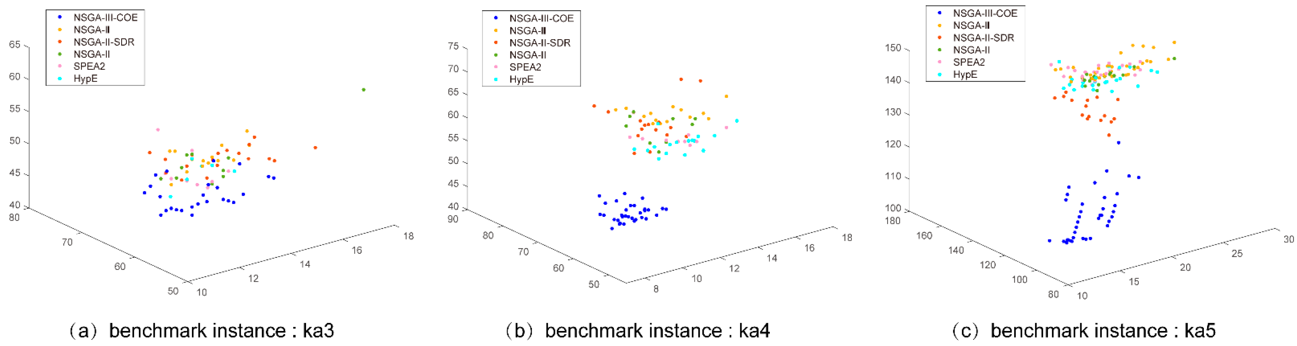
In order to study the search performance of all NSGA-III variant algorithms in the decision space, we use part of three sets of well-known FJSP benchmark instances, including ka3, ka4, and ka5 in the Kacem instance [22] and mk4, mk5, and mk7 in the BRdata instance [21], to conduct exploration and testing. These six instances are representative from simple to complex. In the experiments in this section, we use these six benchmark instances to explore the NSGA-III variants mentioned in this section and propose a modified NSGA-III based on the research results.

Table 3. Parameter setting of the non-dominated sorting genetic algorithm-III (NSGA-III) variant algorithm.

Parameter	Value
Crossover probability ($P_c$)	0.95
Mutation probability ($P_m$)	0.05

lists the parameters used in this section to study the different variants of NSGA-III, and we use uniform parameter values for all variants. In preliminary research, we found that the widely used MOEAs are prone to fall into local optimum on FJSP. Some studies in the literature have found that a larger mutation probability can effectively help the population jump out of the local optimum [10]. Thus, we use a high mutation probability. In order to explore whether the performance of different variants is related to population size, we use two population sizes in our research, 200 and 300. When the number of iterations reaches the set maximum number of iterations, the algorithm is terminated. To ensure a fair comparison, for each benchmark instance, all variants are run independently with the same initial population 30 times, and the average of 30 experiments is taken for comparison.

In our experiments, we use the generational distance (GD) [28] and the inverted generational distance (IGD) [29] as evaluation indicators to evaluate the convergence of the non-dominated solution set and the comprehensive performance of the algorithm. They can be expressed as follows.

GD: Assuming that $P$ is the solution set obtained by the algorithm and $P^{*}$ is a set of uniformly distributed reference points sampled from the Pareto front (PF), the GD of solution set $P$ is defined as follows:

$$GD\left(P,P^{*}\right)=\frac{1}{\left|P\right|}\sqrt{{\displaystyle \sum _{y\in P}\underset{x\in P^{*}}{\min }}\left(dis{(x,y)}^2\right)},$$

(8)

$dis(x,y)$ represents the Euclidean distance between point $y$ in solution set $P$ and point $x$ in reference set $P^{*}$. GD only evaluates the convergence of the solution set. The smaller the GD value is, the better the convergence of the algorithm is.

IGD: Assuming that $P$ is the solution set obtained by the algorithm and $P^{*}$ is a set of uniformly distributed reference points sampled from the Pareto front (PF), then the IGD value of solution set $P$ is defined as follows:

$$IGD\left(P,P^{*}\right)=\frac{1}{\left|P^{*}\right|}{\displaystyle \sum _{x\in P^{*}}\underset{y\in P}{\min }} dis(x,y),$$

(9)

$dis(x,y)$ represents the Euclidean distance between point $x$ in reference set $P^{*}$ and point $y$ in solution set $P$. If $\left|P^{*}\right|$ is large enough to fully represent the Pareto front, then the IGD can comprehensively measure the convergence and the diversity of the solution set. If we want to obtain a smaller IGD, the solution set must be close enough to the Pareto front in the target space.

When calculating the GD and the IGD, a reference set is needed. Since the actual Pareto front of the benchmark instance is unknown, the reference set used in the calculation of the GD and the IGD in this paper is formed by collecting all the non-dominated solutions found during the runtime of all implemented algorithms.

Next, we compare the search behavior of different NSGA-III variants on the MO-FJSP. Simply put, we want to understand the algorithm search process for solution sets in the decision space as well as which algorithm is better at exploration and which algorithm is better at development. Knowing these can help us design more effective evolutionary mechanisms. First, we randomly initialize a population for each instance and then perform 200 and 300 iterations.

Figure 2 and Figure 3 depicts the trajectories of the GDs obtained from the six NSGA-III variants as the number of iterations increases when the population sizes are 200 and 300, respectively. Figure 2 and Figure 3 show that, although the population sizes are different, the same NSGA-III variant shows very similar convergence trends on these benchmark instances, and the convergence of different NSGA-III variants is significantly different due to the different complexities of the benchmark instances. As the complexity of the benchmark instance increases, NSGA-III-CX, NSGA-III-OBX, and NSGA-III-PBX show better convergence, and the GDs of these three algorithms decrease in a similar way during the evolutionary process. This phenomenon indicates that the initial population is a randomly distributed solution in the decision space, and then the optimal solution is searched continuously. NSGA-III-CX, NSGA-III-OBX, and NSGA-III-PBX can search for better solutions faster than other algorithms. The above experimental results show that the three NSGA-III variants, NSGA-III-CX, NSGA-III-OBX, and NSGA-III-PBX, can explore more optimal solutions more effectively in the decision space.

In order to study the development capabilities of different NSGA-III variants, we conduct a similar experiment. The difference from the previous experiment is that we replace the initial population with a population that is already closer to the Pareto front, which can be obtained through iteration by any multi-objective evolutionary algorithm. In this experiment, only the three NSGA-III variants with better exploration capabilities are used. The purpose is to study the abilities of NSGA-III-CX, NSGA-III-OBX, and NSGA-III-PBX to develop better solutions. The three NSGA-III variant algorithms use the population close to the Pareto front as the initial population to perform 100 iterations. As before, use two population sizes, 200 and 300.

Figure 4 and Figure 5 depicts the trajectories of IGDs obtained from the three NSGA-III variants as the number of iterations increases when the initial population is close to the Pareto front when the population size is 200 and 300 respectively. We compare Figure 4 and Figure 5 first. Similar to the previous experiment, the same NSGA-III variant showed very similar ability to develop better solutions when the population size was different. However, the situation in Figure 4 and Figure 5 is very different from that in Figure 2 and Figure 3. In Figure 4 and Figure 5, from the beginning, as the number of iterations increases, a certain algorithm will reduce IGD faster, while the IGD of other algorithms will decrease more slowly. Since the initial population is a population closer to the Pareto frontier, an algorithm with a faster IGD decline has a better ability to develop better solutions in the decision space. In Figure 4e and Figure 5e, on the instance mk5, the NSGA-III-CX has the best ability to develop better solutions. NSGA-III-OBX has the best development capability on other instances. It is speculated from this that when faced with different decision spaces, the crossover operator with better development capabilities may change. The research in this section can help us design more effective evolutionary mechanisms to solve low carbon FJSP.

3.3. The NSGA-III-COE Proposal

The research in the previous two sections shows that the NSGA-III variant using the three crossover operators CX, OBX, and PBX has better exploration capabilities than others in the decision space. When the initial population is close to the Pareto frontier, in most instances, NSGA-III-OBX has the best ability to develop better solutions in the decision space. However, in a few instances, NSGA-III-OBX does not have the best development capabilities. Therefore, which cross-operator has the best development capability is still uncertain. The above research aims to help us design a more effective evolutionary mechanism when solving the MO-FJSP.

Many studies have shown that exploring and developing strategies at the same time can find more useful information from the decision space in the process of finding a better solution. If we make full use of the three crossover operators of CX, OBX, and PBX, we can expect the algorithm to achieve better performance. This is the motivation for proposing the NSGA-III-COE algorithm. The effects of three different crossover operators are naturally integrated to improve the search ability of the decision space and maintain the diversity of the population. This is the main purpose of the NSGA-III-COE.

The NSGA-III-COE is the result of the combination of Pareto dominance and indicator-based thought. In order to achieve our purpose, we decided to coevolve three subpopulations using CX, OBX, and PBX crossover operators. In the process of evolution, natural selection is carried out by simulating the evolution of biological populations to achieve the purpose of survival of the fittest. To achieve natural selection, a certain parameter is necessary to guide the evolution of the population. Therefore, we combine the indicator-based idea with NSGA-III and add the concept of indicator into NSGA-III to guide the natural selection of the population.

In order to propose the NSGA-III-COE algorithm, we introduce the set coverage (SC) [30]. Assuming that both set A and set B are obtained approximate solution sets, the numerator of formula (10) represents the number of solutions in which the solution in B is dominated by at least one solution in A, and the denominator represents the total number of solutions contained in B. The SC is the probability that the solutions in B is dominated by at least one solution in A.

$$C\left(A,B\right)=\frac{\left|\left\{x\in B|\exists y\in A:y \mathrm{dominates} x\right\}\right|}{\left|B\right|},$$

(10)

Each subpopulation in the initial population has the same number of individuals. In the evolution process, the evolution of biological populations is simulated, and a small number of individuals are randomly exchanged in each iteration to increase the diversity of chromosomes in the decision space and to increase the amount of useful information in the decision space.

When the evolution reaches half of the maximum number of iterations, the SC indicator intervenes. The subpopulation size is adjusted every 10 generations according to the SC indicator. The SC indicator makes natural selection of the subpopulation based on the exploration and the development ability of the subpopulation in the decision space. Natural selection in the evolutionary process means increasing the size of superior subpopulations and reducing the size of disadvantaged subpopulations in order to achieve the survival of the fittest. Algorithm 1 describes the evolutionary mechanism of the NSGA-III-COE.

Algorithm 1: Evolutionary mechanism of the NSGA-III-COE.

1.       function Evolution(PopCX, PopOBX, PopPBX, genNow, gen)

2.               if genNow > gen/2 and mod(genNow, gen/10) == 0 then

3.                    PopCX, PopOBX, PopPBX $\leftarrow$ AdjustPopSzie(PopCX, PopOBX, PopPBX)

4.               end if

5.               PopCX, PopOBX, PopPBX $\leftarrow$ RandomExchange(PopCX, PopOBX, PopPBX)

6.               PopCX $\leftarrow$ OperatorCX(PopCX)

7.               PopCX $\leftarrow$ OperatorCX(PopCX)

8.               PopCX $\leftarrow$ OperatorCX(PopCX)

9.               return PopCX, PopOBX, PopPBX

10.      end function

4. Experimental Results and Discussion

In order to verify the advantages of the NSGA-III-COE in the MO-FJSP decision space exploration and development capabilities, a large number of computational experiments were carried out. These experiments were implemented by MATLAB programming and were tested on three sets of well-known benchmark instances, including 5 Kacem instances (ka1, ka2, ka3, ka4, ka5) [22], 10 BRdata instances (mk1–mk10) [21], and 12 BRdata instances (01a–12a) [22]. These collections cover most of the problem instances used in the FJSP literature. In fact, most of the existing research only considers a small part of them. In our experiment, 27 instances are used to comprehensively evaluate the algorithm we propose.

Table 4. Experimental parameter settings for the co-evolutionary NSGA-III (NSGA-III-COE) performance evaluation.

Parameter	Value
Population size ($N$)	300
Initial size of each subpopulation ($N_s$)	100
Number of objectives ($M$)	3
Maximum number of iterations ($T_{\max }$)	300
Crossover probability ($P_c$)	0.95
Mutation probability ($P_m$)	0.05

lists the parameter settings of the algorithm, and we use uniform parameter values for the algorithm. For all instances, the maximum number of iterations is set to 300, and it is the same for all implemented algorithms. When the number of iterations reaches the set maximum number of iterations, the algorithm terminates to ensure fair comparison. For each instance, all algorithms run independently 30 times starting with the same initial population.

We are not sure whether all the nondominant solutions of the 27 benchmark instances collected in this paper enable IGD to more accurately reflect the overall performance of the algorithm on all instances. Therefore, this paper uses the hypervolume (HV) [30] indicator to evaluate the overall performance of the algorithms for all 27 instances.

Suppose $P$ is the solution set obtained by the algorithm, and $q={\left(q_1,q_2,\cdots ,q_m\right)}^T$ is a reference point in the target space, which is dominated by all the target vectors in the solution set $P$. Then, the HV for reference point $q$ refers to the volume of the target space dominated by solution set $P$ and bounded by reference point $q$.

$$HV\left(P,q\right)=\mathrm{volume}\left(\underset{p\in P}{\cup }[p_1,q_1]\times [p_2,q_2]\cdots [p_m,q_m]\right),$$

(11)

Figure 6 illustrates the meaning of HV in a two-dimensional target space. The HV indicator calculation does not require a reference point set and can comprehensively reflect the convergence and the diversity of the solution set. The larger the HV is, the better the solution set obtained by the algorithm is and the better the overall performance of the algorithm will be.

4.1. Comparison of NSGA-III-COE and NSGA-III Variants

In this section, we compare the NSGA-III-COE with NSGA-III-CX, NSGA-III-OBX, and NSGA-III-PBX to verify whether the population evolution mechanism proposed in this paper can integrate the effects of the three different crossover operators, enhance exploration and development capabilities in the decision space, and improve the performance of the algorithm.

Table 5. Performance evaluation of NSGA-III-COE, NSGA-III-CX (cycle crossover), NSGA-III-OBX (order-based crossover), and NSGA-III-PBX (partially mapped crossover); the average HVs of 27 problem cases running independently 30 times. For each instance, the results which are better than the others are marked in bold (these have the largest HV value).

Instance	${\mathit{N}}_{\mathit{n}}\times {\mathit{N}}_{\mathit{m}}$	NSGA-III-COE	NSGA-III-CX	NSGA-III-OBX	NSGA-III-PBX
ka1	3 × 4	0.038924	0.038924	0.038924	0.038924
ka2	4 × 5	0.026456	0.025696	0.026089	0.026372
ka3	10 × 7	0.036638	0.032826	0.036285	0.032998
ka4	10 × 10	0.052563	0.040711	0.043659	0.043500
ka5	15 × 10	0.024589	0.017029	0.022309	0.018040
mk1	10 × 6	0.030030	0.027031	0.029851	0.027547
mk2	10 × 6	0.055304	0.044472	0.049948	0.046155
mk3	15 × 8	0.010112	0.007421	0.007984	0.006651
mk4	15 × 8	0.005349	0.004029	0.003676	0.003089
mk5	15 × 4	0.002695	0.001993	0.001973	0.001895
mk6	10 × 15	0.005967	0.005599	0.004701	0.004495
mk7	20 × 5	0.005084	0.003309	0.004169	0.002962
mk8	20 × 10	0.003186	0.002989	0.002653	0.002296
mk9	20 × 10	0.001387	0.000730	0.000938	0.000414
mk10	20 × 15	0.001743	0.001098	0.001048	0.000477
01a	10 × 5	0.008513	0.007916	0.007997	0.008070
02a	10 × 5	0.003472	0.003414	0.003424	0.003472
03a	10 × 5	0.007070	0.005914	0.006099	0.005359
04a	10 × 5	0.004745	0.004028	0.004182	0.004116
05a	10 × 5	0.005202	0.004891	0.004659	0.004669
06a	10 × 5	0.008040	0.007375	0.007533	0.007330
07a	15 × 8	0.003521	0.003202	0.002860	0.002810
08a	15 × 8	0.003402	0.003080	0.002755	0.002622
09a	15 × 8	0.007588	0.007092	0.006975	0.006986
10a	15 × 8	0.002659	0.002087	0.001968	0.001715
11a	15 × 8	0.003447	0.003106	0.003053	0.002382
12a	15 × 8	0.001557	0.001222	0.001134	0.000959

shows the normalized average HVs obtained by running four algorithms 30 times independently on 27 benchmark instances. In addition, the features of the instance are also listed in the table. The first column indicates the name of the instance, and the second column indicates the size of the instance, where $N_n$ indicates the number of processes, and $N_m$ indicates the number of machines.

First, we analyze the three algorithms, NSGA-III-CX, NSGA-III-OBX, and NSGA-III-PBX. In 14 instances, the NSGA-III-OBX obtains the largest HV. In 11 instances, the NSGA-III-CX obtains the largest HV, and the NSGA-III-PBX obtains the largest HV in two instances. This phenomenon validates our conjecture when studying the developmental capabilities of NSGA-III variants. The same crossover operator shows different capabilities for developing better solutions when facing different MO-FJSPs.

Then, we add the NSGA-III-COE for analysis. Except for instances ka1 and mk2, the HVs of the NSGA-III-COE in the remaining 25 instances are all larger than those of the other NSGA-III variants. In instance ka1, the four algorithms have the same HVs. In instance mk2, NSGA-III-COE and NSGA-III-PBX both have the largest HVs. With the increase of instance complexity, the HV value of the NSGA-III-COE increases more and more obviously than other algorithms. This shows that the NSGA-III-COE performs best in all 27 instances, and as the complexity of the instance increases, the NSGA-III-COE shows better performance.

In order to further verify whether the evolutionary mechanism proposed in this paper reaches our original design intention, Figure 7 shows the performances of the four algorithms of NSGA-III-COE, NSGA-III-CX, NSGA-III-OBX, and NSGA-III-PBX in instance mk2–mk10 at obtaining the non-dominated solution set in the same coordinate system obtained above. It can be seen from the figure that the non-dominated solution set obtained by the NSGA-III-COE is closer to the Pareto frontier than the other three algorithms and has good diversity. This indicates that the evolutionary mechanism proposed in this paper enhances search and development capabilities in the MO-FJSP decision space and speeds up the convergence speed while maintaining the diversity of the population, thus the algorithm obtains better performance.

4.2. Comparison of the NSGA-III-COE with Widely Used MOEAs

This section compares the NSGA-III-COE with the existing widely used MOEAs. NSGA-III, NSGA-II, NSGA-II/strengthened dominance relation(NSGA-II/SDR) [31], improving the strength pareto evolutionary algorithm (SPEA2) [32] and hypervolume estimation algorithm for multi-objective optimization (HypE) [33] are chosen as the comparison algorithms because they are all currently widely used MOEAs that can be directly applied to solve the MO-FJSP after simple modification, and some of them have been used many times in the previous FJSP literature. Ahmadi et al. [34] used the NSGA-II to solve the FJSP with random failures. Bandyopadhyay et al. [10] compared the calculation results with NSGA-II and SPEA2 when solving a parallel machine scheduling problem. Yuan Y et al. [9] also used the NSGA-II for comparison when solving the FJSP. NSGA-II is used very frequently in solving scheduling problems. Therefore, this paper adds the newer modified NSGA-II algorithm NSGA-II/SDR to the comparison algorithms.

Table 6. Performance evaluation of the NSGA-III-COE and other comparison algorithms; the average HVs of 27 problem instances running 30 times independently. For each instance, the results which are significantly better than the others are marked in bold (these have much larger HV value than the other algorithms).

Instance	NSGA-III-COE	NSGA-III	NSGA-II/SDR	NSGA-II	SPEA2	HypE
ka1	0.038917	0.038763	0.038318	0.038678	0.038736	0.038609
ka2	0.026269	0.020522	0.020711	0.020292	0.023692	0.019619
ka3	0.014032	0.002858	0.002535	0.003239	0.002040	0.002653
ka4	0.073033	0.006564	0.007325	0.006934	0.005123	0.008142
ka5	0.045579	0.000723	0.001969	0.000670	0.000588	0.000775
mk1	0.027291	0.018659	0.018743	0.018591	0.017901	0.019043
mk2	0.085445	0.021139	0.023545	0.019240	0.015013	0.019672
mk3	0.055143	0.002332	0.002295	0.002367	0.002356	0.002455
mk4	0.031763	0.002991	0.003800	0.003022	0.003653	0.002835
mk5	0.014355	0.005375	0.005355	0.005334	0.006319	0.005436
mk6	0.069930	0.002379	0.003002	0.002544	0.004145	0.002644
mk7	0.043737	0.000740	0.001216	0.000716	0.000538	0.000610
mk8	0.020138	0.004515	0.003760	0.004417	0.004931	0.004724
mk9	0.043676	0.002392	0.002172	0.002298	0.003155	0.002507
mk10	0.039108	0.001319	0.001241	0.001250	0.001844	0.001281
01a	0.018298	0.003541	0.002632	0.003667	0.004244	0.003577
02a	0.022695	0.005291	0.004244	0.005345	0.006299	0.005265
03a	0.056274	0.008078	0.006250	0.008256	0.008777	0.008300
04a	0.024167	0.003110	0.002453	0.003039	0.003906	0.003125
05a	0.031675	0.004629	0.003988	0.004528	0.005552	0.004746
06a	0.016381	0.000991	0.000761	0.000875	0.001517	0.000941
07a	0.018122	0.002454	0.001985	0.002615	0.003106	0.002458
08a	0.020696	0.001245	0.001055	0.001240	0.001732	0.001313
09a	0.019022	0.001157	0.000955	0.001201	0.001597	0.001191
10a	0.022589	0.003136	0.002363	0.003140	0.003853	0.003125
11a	0.032415	0.002615	0.002055	0.002671	0.003192	0.002660
12a	0.022939	0.001854	0.001272	0.001954	0.002330	0.001810

shows the average HVs for 30 independent runs on 27 instances of NSGA-III-COE, NSGA-III, NSGA-II, NSGA-II/SDR, SPEA2, and HypE. The table shows that the HVs of the NSGA-III-COE on the three instances of ka1, ka2, and mk1 are slightly larger than those of the other algorithms. On the remaining 24 instances, the HVs of the NSGA-III-COE are much larger than those of the other algorithms. As the complexity of the benchmark instances increases, the advantages of the NSGA-III-COE become increasingly more obvious.

Figure 8, Figure 9 and Figure 10 show the non-dominated solution set in the same coordinate system obtained by the NSGA-III-COE and the comparison algorithm used in this section on almost all benchmark instances. It can be seen from the figure that the performance of the original NSGA-III is relatively close to that of other comparison algorithms. However, the non-dominated solution sets obtained by all the comparison algorithms are far away from the Pareto front, which obviously falls into the local optimum. The non-dominated solution obtained by the NSGA-III-COE is far superior to other comparison algorithms. This shows that the population evolution mechanism proposed in this paper is not only conducive to the improvement of convergence speed but also improves the ability to jump out of the local optimum on the MO-FJSP and greatly improves the performance of NSGA-III in solving the MO-FJSP.

We count the running time of six algorithms on 27 instances, and the results are shown in Figure 11. The running time of the NSGA-III-COE is slightly longer than that of the NSGA-III. Compared with these widely used MOEAs, the computational cost of the NSGA-III-COE is at a moderate level.

4.3. Sensitivity Analysis of Population Size

In this section, we associate the performance of the NSGA-III-COE and the other five MOEAs with the population size, which ranges from 30 to 500. We study the sensitivity of the NSGA-III-COE to population size on 27 FJSP benchmark instances.

We use SR (sum of ranks) to represent the performance of the algorithm:

$$SR=ran{k}_{\mathrm{ka}1}+\dots +ran{k}_{\mathrm{ka}5}+ran{k}_{\mathrm{mk}1}+\dots +ran{k}_{\mathrm{mk}10}+ran{k}_{01\mathrm{a}}+\dots +ran{k}_{12\mathrm{a}},$$

(12)

where $rank$ represents the ranking of an algorithm among all algorithms for a benchmark instance. The ranking of the algorithm is based on the HV value of the non-dominated solution set. The larger the HV value is, the smaller the SR is, which means a higher ranking. For example, $ran{k}_{\mathrm{ka}1}$ represents the ranking of an algorithm on instance ka1. $SR$ represents the cumulative sum rankings of an algorithm on all instances.

From Figure 12, the following experimental observation results can be obtained.

• In experiments of different population sizes, the NSGA-III-COE achieves the highest ranking and is considerably ahead of other algorithms.
• Some comparative MOEAs show sensitivity to population size. The most obvious is that the SPEA2 ranks best when the population size is 100.
• In this set of comparative experiments, the NSGA-III-COE does not show obvious sensitivity to population size, and it performs well in the seven population sizes.

Considering experimental results, running time, and sensitivity to population size, the NSGA-III-COE is a very competitive algorithm for solving low carbon FJSP.

5. Conclusions

In this paper, a low carbon MO-FJSP mathematical model is established to minimize total completion time, total carbon emissions, and total machine load. This mathematical model is very close to the real production environment and conforms to the concepts of green manufacturing and sustainable development. By understanding the existing literature on the MO-FJSP research, this paper introduces five crossover operators into the NSGA-III to produce different NSGA-III variants. Then, the ability of different NSGA-III variants to explore and develop better solutions in the decision space on some FJSP benchmark instances is studied. Through research and analysis of the experimental results, the indicator-based thought is introduced into NSGA-III, and a new co-evolutionary mechanism incorporated with multi-crossover operator and natural selection is proposed, which combines the capabilities of different crossover operators to make the algorithm obtain better performance. Subsequently, we introduce the new evolutionary mechanism into the NSGA-III and propose the NSGA-III-COE. Using the NSGA-III-COE to solve low carbon MO-FJSP, multiple experiments are done. The NSGA-III-COE achieves good results in solving the MO-FJSP.

In the experiment, we compare the NSGA-III-COE with five existing widely used MOEAs on 27 benchmark instances in the three\ test sets of the FJSP. Experimental results show that the NSGA-III-COE has a strong ability to optimize the low carbon MO-FJSP, and the computational cost of solving the problem is similar to that of widely used MOEAs. Compared with other widely used algorithms, the NSGA-III-COE algorithm has obvious advantages in convergence speed and the ability to jump out of local optimum. Especially, it shows better performance when dealing with complex problem cases. Since the solving time of FJSP increases exponentially with the increase of the problem scale, our research is very meaningful for solving the low carbon MO-FJSP.

The work done in this paper only shows that the proposed the NSGA-III-COE is effective for solving the MO-FJSP. In the future, we will further study the production scheduling problem, continue to research and improve the algorithm, and apply the algorithm to solve other multi-objective production scheduling problems.

References

1. Cinar, D.; Oliveira, J.A.; Topcu, Y.I.; Pardalos, P.M. A priority-based genetic algorithm for a flexible job scheduling problem. J. Ind. Manag. Optim. 2017, 12, 1391–1415. [Google Scholar] [CrossRef]
2. Bozejko, W.; Uchronski, M.; Wodecki, M. Parallel hybrid metaheuristics for the flexible job problem. Comput. Ind. Eng. 2010, 59, 323–333. [Google Scholar] [CrossRef]
3. Jamrus, T.; Chien, C.F.; Gen, M.; Sethanan, K. Hybrid particle swarm optimization combined with genetic operators for flexible job-shop scheduling under uncertain processing time for semiconductor manufacturing. IEEE Trans. Semicond. Manuf. 2017, 31, 32–41. [Google Scholar] [CrossRef]
4. Yuan, Y.; Xu, H.; Yang, J. A hybrid harmony search algorithm for the flexible job scheduling problem. Appl. Soft Comput. J. 2013, 13, 3259–3272. [Google Scholar] [CrossRef]
5. Wu, X.; Wu, S. An elitist quantum-inspired evolutionary algorithm for the flexible job-shop scheduling problem. J. Intell. Manuf. 2017, 28, 1441–1457. [Google Scholar] [CrossRef] [Green Version]
6. Hmida, A.B.; Haouari, M.; Huguet, M.J.; Lopez, P. Discrepancy search for the flexible job scheduling problem. Comput. Oper. Res. 2010, 37, 2192–2201. [Google Scholar] [CrossRef] [Green Version]
7. Deb, K.; Pratap, A.; Agarwal, S.; Meyarivan, T. A fast and elitist multi-objective genetic algorithm: NSGA-II. IEEE Trans. Evol. Comput. 2002, 6, 182–197. [Google Scholar] [CrossRef] [Green Version]
8. Jiang, Z.Q.; Zuo, L. Multi-objective flexible job-shop scheduling based on low carbon strategy. Comput. Integr. Manuf. Syst. 2015, 21, 1023–1031. [Google Scholar]
9. Yuan, Y.; Xu, H. Multi-objective Flexible Job Scheduling Using Memetic Algorithms. IEEE Trans. Autom. Sci. Eng. 2014, 12, 336–353. [Google Scholar] [CrossRef]
10. Bhattacharya, B.R. Solving multi-objective parallel machine scheduling problem by a modified NSGA-II. Appl. Math. Model. 2013, 37, 6718–6729. [Google Scholar]
11. Zhao, B.; Gao, J.; Chen, K.; Guo, K. Two-generation Pareto ant colony algorithm for multi-objective job scheduling problem with alternative process plans and unrelated parallel machines. J. Intell. Manuf. 2018, 29, 93–108. [Google Scholar] [CrossRef]
12. Piroozfard, H.; Wong, K.Y.; Wong, W.P. Minimizing total carbon footprint and total late work criterion in flexible job scheduling by using an improved multi-objective genetic algorithm. Resour. Conserv. Recycl. 2018, 128, 267–283. [Google Scholar] [CrossRef]
13. Pomar, L.A.; Pulido, E.C.; Roa, J.D.T. A Hybrid Genetic Algorithm and Particle Swarm Optimization for Flow Shop Scheduling Problems. In Proceedings of the Workshop on Engineering Applications, Cartagena, CA, USA, 27–29 September 2017; pp. 601–612. [Google Scholar]
14. Burdett, R.L.; Kozan, E. An integrated approach for scheduling health care activities in a hospital. Eur. J. Oper. Res. 2018, 264, 756–773. [Google Scholar] [CrossRef] [Green Version]
15. Burdett, R.L.; Corry, P.; Yarlagadda, P.K.; Eustace, C.; Smith, S. A flexible job shop scheduling approach with operators for coal export terminals. Comput. Oper. Res. 2019, 104, 15–36. [Google Scholar] [CrossRef]
16. Mansouri, S.A.; Aktas, E.; Besikci, U. Green scheduling of a two-machine flowshop: Trade-off between makespan and energy consumption. Eur. J. Oper. Res. 2015, 248, 772–788. [Google Scholar] [CrossRef] [Green Version]
17. Mokhtari, H.; Hasani, A. An Energy-Efficient Multi-Objective Optimization for Flexible Job-Shop Scheduling Problem. Comput. Chem. Eng. 2017, 104, 339–352. [Google Scholar] [CrossRef]
18. Lu, C.; Li, X.; Gao, L.; Liao, W.; Yi, J. An effective multi-objective discrete virus optimization algorithm for flexible job-shop scheduling problem with controllable processing times. Comput. Ind. Eng. 2017, 104, 156–174. [Google Scholar] [CrossRef]
19. Ding, J.Y.; Song, S.; Wu, C. Carbon-efficient scheduling of flow shops by multi-objective optimization. Eur. J. Oper. Res. 2015, 248, 758–771. [Google Scholar] [CrossRef]
20. Deb, K.; Jain, H. An Evolutionary Many-Objective Optimization Algorithm Using Reference-Point-Based Non-dominated Sorting Approach, Part I: Solving Problems with Box Constraints. IEEE Trans. Evol. Comput. 2014, 18, 577–601. [Google Scholar] [CrossRef]
21. Brandimarte, P. Routing and scheduling in a flexible job by tabu search. Ann. Oper. Res. 1993, 41, 157–183. [Google Scholar] [CrossRef]
22. Kacem, I.; Hammadi, S.; Borne, P. Pareto-optimality approach for flexible job-shop scheduling problems: Hybridization of evolutionary algorithms and fuzzy logic. Math. Comput. Simul. 2014, 60, 245–276. [Google Scholar] [CrossRef]
23. Agrawal, R.B.; Deb, K.; Agrawal, R.B. Simulated Binary Crossover for Continuous Search Space. Complex Syst. 1994, 9, 115–148. [Google Scholar]
24. Oliver, I.M.; Smith, D.J.; Holland, J.R.C. A Study of Permutation Crossover Operators on the Traveling Salesman Problem. In Proceedings of the Second International Conference on Genetic Algorithms on Genetic Algorithms and Their application, Cambridge, MA, USA, 28–31 July 1987; pp. 224–230. [Google Scholar]
25. Syswerda, G. Schedule Optimization Using Genetic Algorithms. In Proceedings of the 4th International Conference on Genetic Algorithms, San Diego, CA, USA, 13–16 July 1991; pp. 94–101. [Google Scholar]
26. Davis, L. Applying adaptive algorithms to epistatic domains. In Proceedings of the International Joint Conference on Artificial Intelligence, Los Angeles, CA, USA, 18–24 August 1985; pp. 162–164. [Google Scholar]
27. Goldberg, D.; Lingle, R. Alleles, loci and the tsp en. In Proceedings of the First International Conference on Genetic Algorithms; Lawrence Erlbaum Associates: Hilldale, NJ, USA, 1985; pp. 154–159. [Google Scholar]
28. Veldhuizen, D.A.V. Multi-Objective Evolutionary Algorithms: Classifications, Analyses, and New Innovations; Air Force Institute of Technology: Wright-Patterson AFB, OH, USA, 1999; pp. 235–243. [Google Scholar]
29. Coello, C.A.C.; Cortes, N.C. Solving Multi-objective Optimization Problems Using an Artificial Immune System. Genet. Program. Evolvable Mach. 2005, 6, 163–190. [Google Scholar] [CrossRef]
30. Zitzler, E.; Thiele, L. Multi-objective evolutionary algorithms: A comparative case study and the strength Pareto approach. IEEE Trans. Evol. Comput. 1999, 3, 257–271. [Google Scholar] [CrossRef] [Green Version]
31. Tian, Y.; Cheng, R.; Zhang, X.; Su, Y.; Jin, Y. A strengthened dominance relation considering convergence and diversity for evolutionary many-objective optimization. IEEE Trans. Evol. Comput. 2019, 23, 331–345. [Google Scholar] [CrossRef] [Green Version]
32. Zitzler, E.; Laumanns, M.; Thiele, L. SPEA2: Improving the strength pareto evolutionary algorithm. TIK-Report 2002, 103, 742–751. [Google Scholar]
33. Bader, J.; Zitzler, E. HypE: An Algorithm for Fast Hypervolume-Based Many-Objective Optimization. Evol. Comput. 2011, 19, 45–76. [Google Scholar] [CrossRef]
34. Ahmadi, E.; Zandieh, M.; Farrokh, M.; Emami, S.M. A multi objective optimization approach for flexible job scheduling problem under random machine breakdown by evolutionary algorithms. Comput. Oper. Res. 2016, 73, 56–66. [Google Scholar] [CrossRef]
Figure 1. Chromosome decoding corresponds to the Gantt chart.
Processes 09 00062 g001
Figure 2. At population size of 200, the evolutionary trajectory of the generational distances (GDs) of the NSGA-III variants on the six FJSP instances (the average of the results of 30 independent runs; the initial population is a random population).
Processes 09 00062 g002
Figure 3. At population size of 300, the evolutionary trajectory of the GDs of the NSGA-III variants on the six FJSP instances (the average of the results of 30 independent runs; the initial population is a random population).
Processes 09 00062 g003
Figure 4. At population size of 200, the evolutionary trajectory of the inverted generational distance (IGD) for the NSGA-III variants on the six FJSP instances (the average of the results of 30 independent runs; the initial population is the population close to the Pareto front in the target space).
Processes 09 00062 g004
Figure 5. At population size of 300, the evolutionary trajectory of the IGD for the NSGA-III variants on the six FJSP instances (the average of the results of 30 independent runs; the initial population is the population close to the Pareto front in the target space).
Processes 09 00062 g005
Figure 6. Diagram of the hypervolume (HV).
Processes 09 00062 g006
Figure 7. The non-dominated solutions of NSGA-III-COE, NSGA-III-CX, NSGA-III-OBX, and NSGA-III-PBX on instances mk2–mk10.
Processes 09 00062 g007
Figure 8. The non-dominated solutions of NSGA-III-COE, NSGA-III, NSGA-II, NSGA-II/SDR, SPEA2, and HypE on instances ka3, ka4, and ka5.
Processes 09 00062 g008
Figure 9. The non-dominated solutions of NSGA-III-COE, NSGA-III, NSGA-II, NSGA-II/SDR, SPEA2, and HypE on instances mk2–mk10.
Processes 09 00062 g009
Figure 10. The non-dominated solutions of NSGA-III-COE, NSGA-III, NSGA-II, NSGA-II/SDR, SPEA2, and HypE on instances 01a–12a.
Processes 09 00062 g010
Figure 11. Average CPU time (in seconds) consumed by NSGA-III-COE and other comparison algorithms on 27 problem instances.
Processes 09 00062 g011
Figure 12. The impact of population size on the performance of the NSGA-III-COE and other multi-objective evolutionary algorithms (MOEAs) on 27 benchmark instances. The figure shows the sum of rankings of 27 instances obtained by each algorithm when the population size is 30, 60, 100, 200, 300, 400, and 500.
Processes 09 00062 g012