Evolutionary Algorithm to Support Field Architecture Scenario Screening Automation and Optimization Using Decentralized Subsea Processing Modules
Abstract
1. Introduction
2. Methods
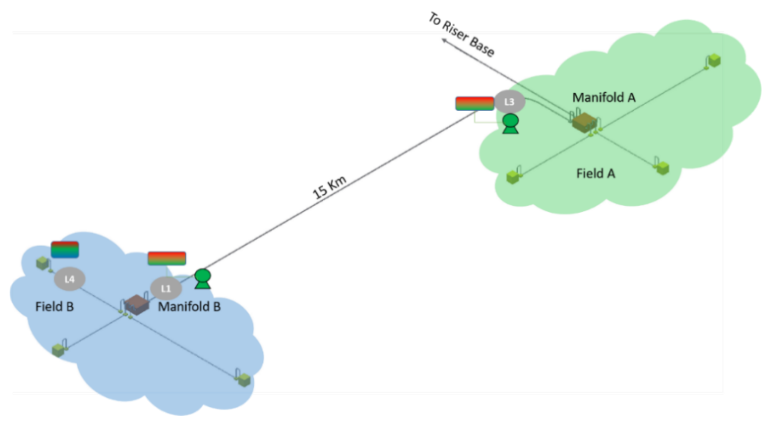
2.1. Problem Statement: The Subsea Gate Box Concept
- location of the SGB within the field
- number of simultaneous SGB within the field
- number of process modules in a SGB
- process train sequence in a SGB
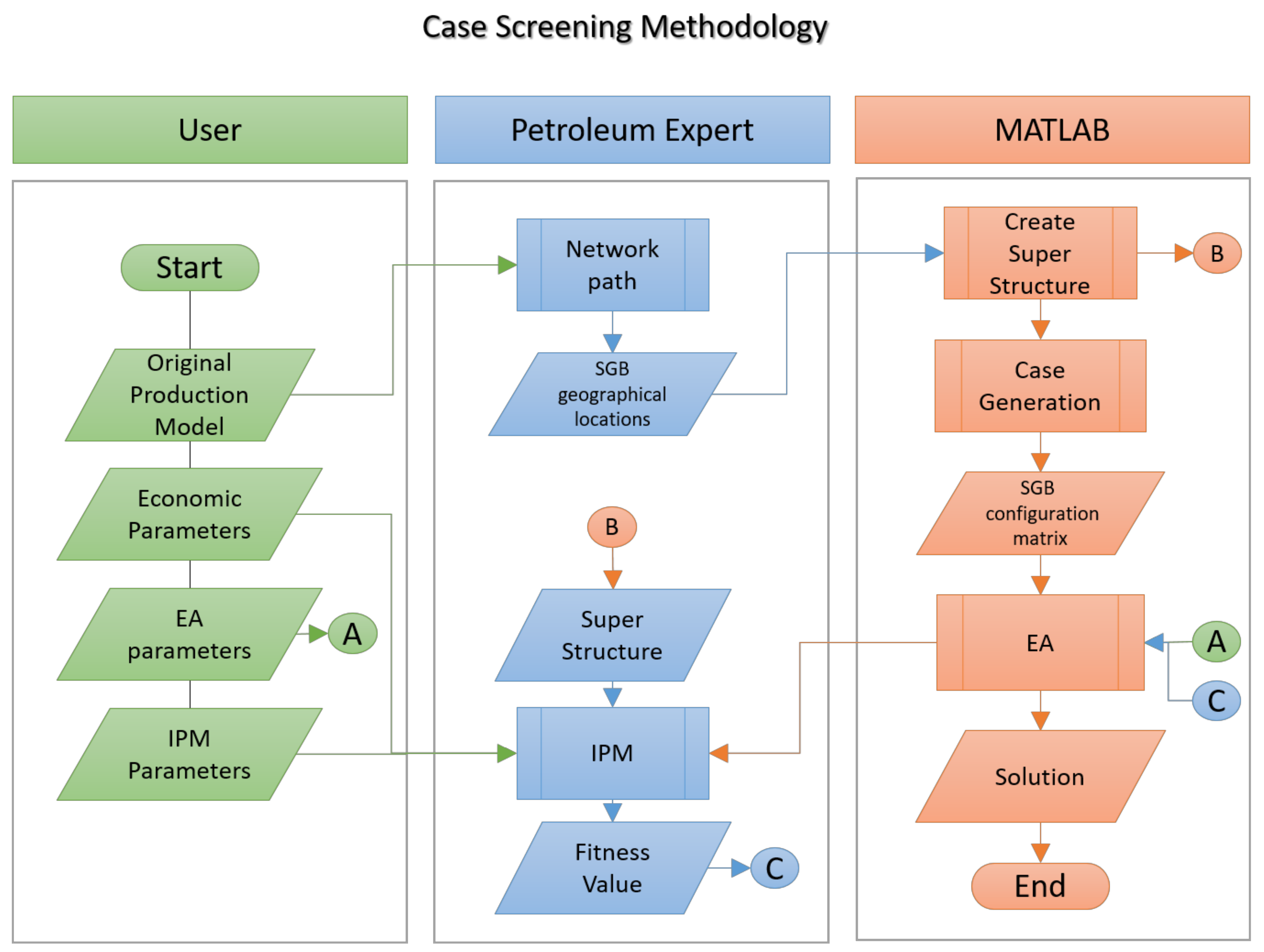
2.2. Case Screening Methodology
- The diameter of the lines remains from the original design, even when the flow rates of the original lines change due to the SGB operation. Likewise, additional lines downstream of separation processes are taken as a copy of the original.
- SGBs are installed at the beginning of the project, and their location, configuration, and the settings of the process modules do not change over time.
- All the optimization settings within the production model are disabled.
- The production model is set to produce to maximum potential.
- The process equipment within the SGB are not fully modeled. The process performances are defined as “nodes” in the network that increase the pressure, split phases, or change the temperature. Therefore, the typical values of efficiency from the literature are used for calculating the power demand and estimating the umbilical requirements.
- The economic model is simplified, as documented in Section 2.5.1.
2.3. Data Collection
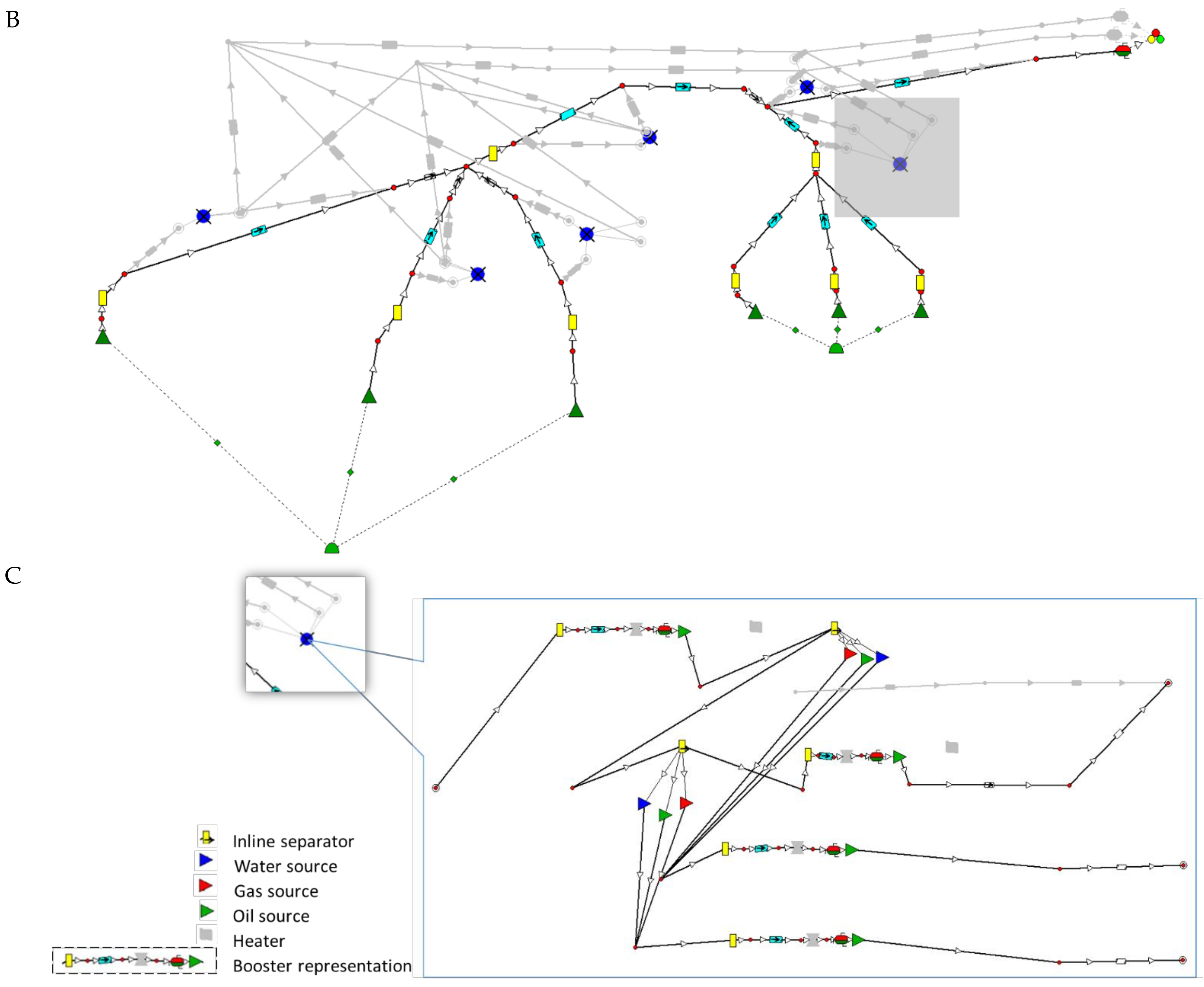
2.4. Identifying Locations and Creating a Superstructure
2.5. The Integrated Model (IPM)
2.5.1. The Fitness Function
- : Net balance at the end of time step t
- : Discount rate
- : Time step into the future
- : Lifetime (project duration) (time step unit)
- : Initial investment outlay
CAPEX Estimation of the SGB (WBS ID: 10101)
- The costs of the pumps and compressors in Table 5 as a function of the mechanical power required at the equipment location and in actual conditions. For this example, it was considered the maximum power demand over the production period as a simplification of the problem (Equation (2)).where:
- Pm: mechanical power
- Ph: hydraulic power
- : pump efficiency
- The hydraulic power for the liquid and multiphase pumps was calculated according to Equation (3) and, for the compressors, according to Equation (4) with 100% polytropic efficiency.where:
- : actual liquid flow rate
- actual gas flow rate
- : discharge pressure
- : suction pressure
- : compression coefficient
- It is assumed that pumps for individual wells achieve higher efficiency than pumps operating at the commingling points. Furthermore, the pumps do not operate at the best efficiency point during the whole production period; therefore, the average efficiency of 55% for the individual streams and 50% for the comingled points are considered in the case of multiphase pumps and 75% and 70% in the case of liquid pumps and compressors, respectively.
- The costs database only included subsea multiphase pumps. Therefore, the costs of the liquid pumps and the compressors are calculated using the multiphase pump price multiplied by a design factor (Equations (5)–(7)). This design factor aims to differentiate among the complexity of the three types of boosters. Thus, the liquid pumps are assumed to be less complex (less expensive) than the multiphase pumps, while the compressors are assumed to be more complex (more expensive) than the multiphase pumps.where the pump price is the “Pump and motor” item in Table 5. The largest motor is assumed to be 3000 kw. For higher power requirements, several pumps in a series or parallel are considered.
- For each booster system (single or parallel/series boosters), one extra spare equipment is considered.
- The costs for separators and heaters units are estimated based on Equation (8)where
- : estimated cost of capacity required
- : the known cost of a given capacity
- x: cost-capacity factor (x = 0.6 for this work)
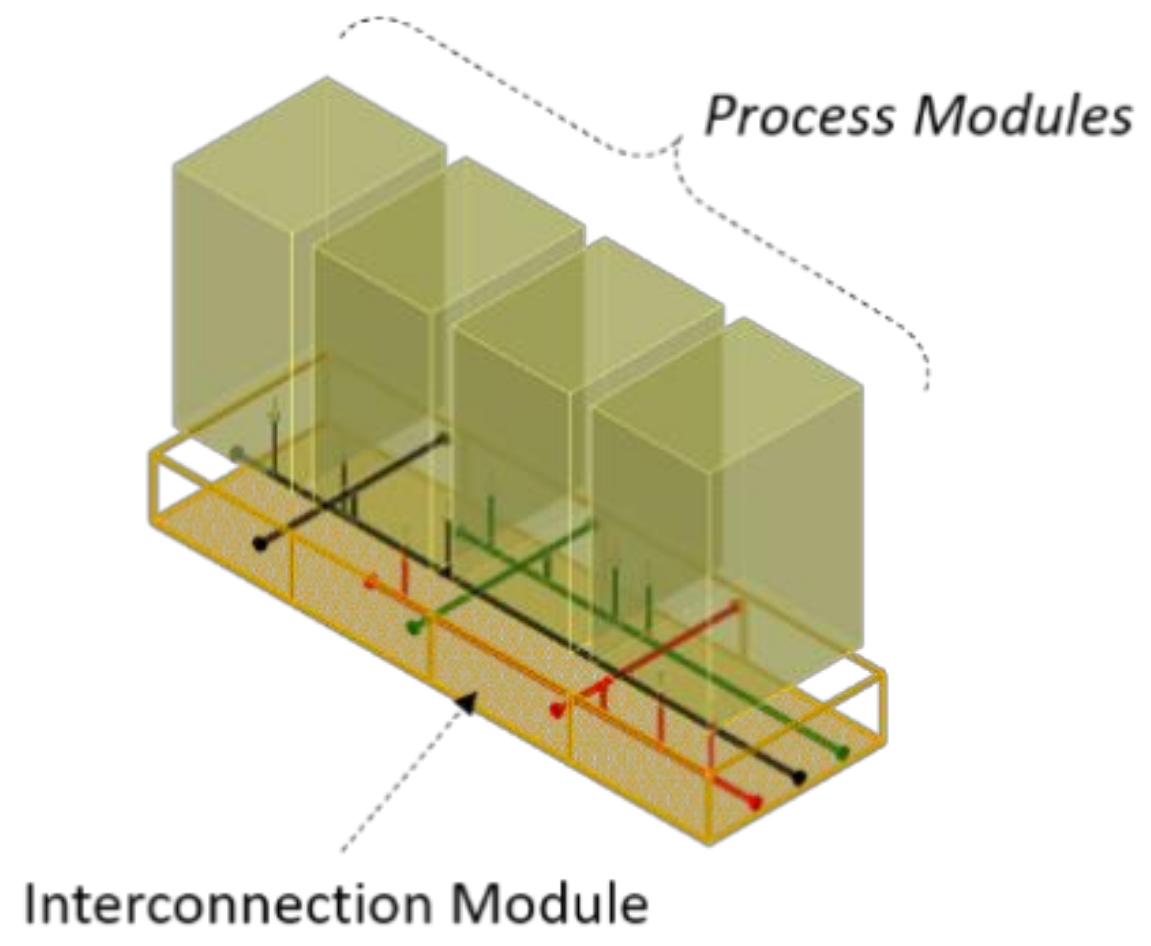
- Interconnection module.
- Flowlines and umbilical
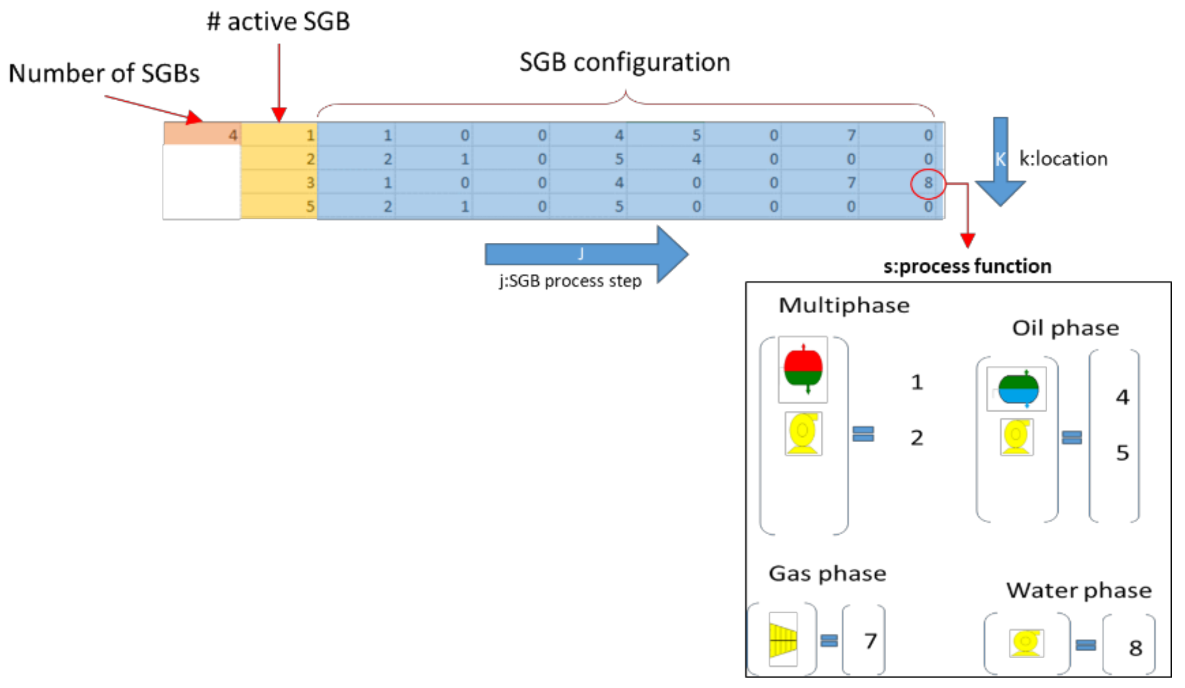
2.6. Case Generation
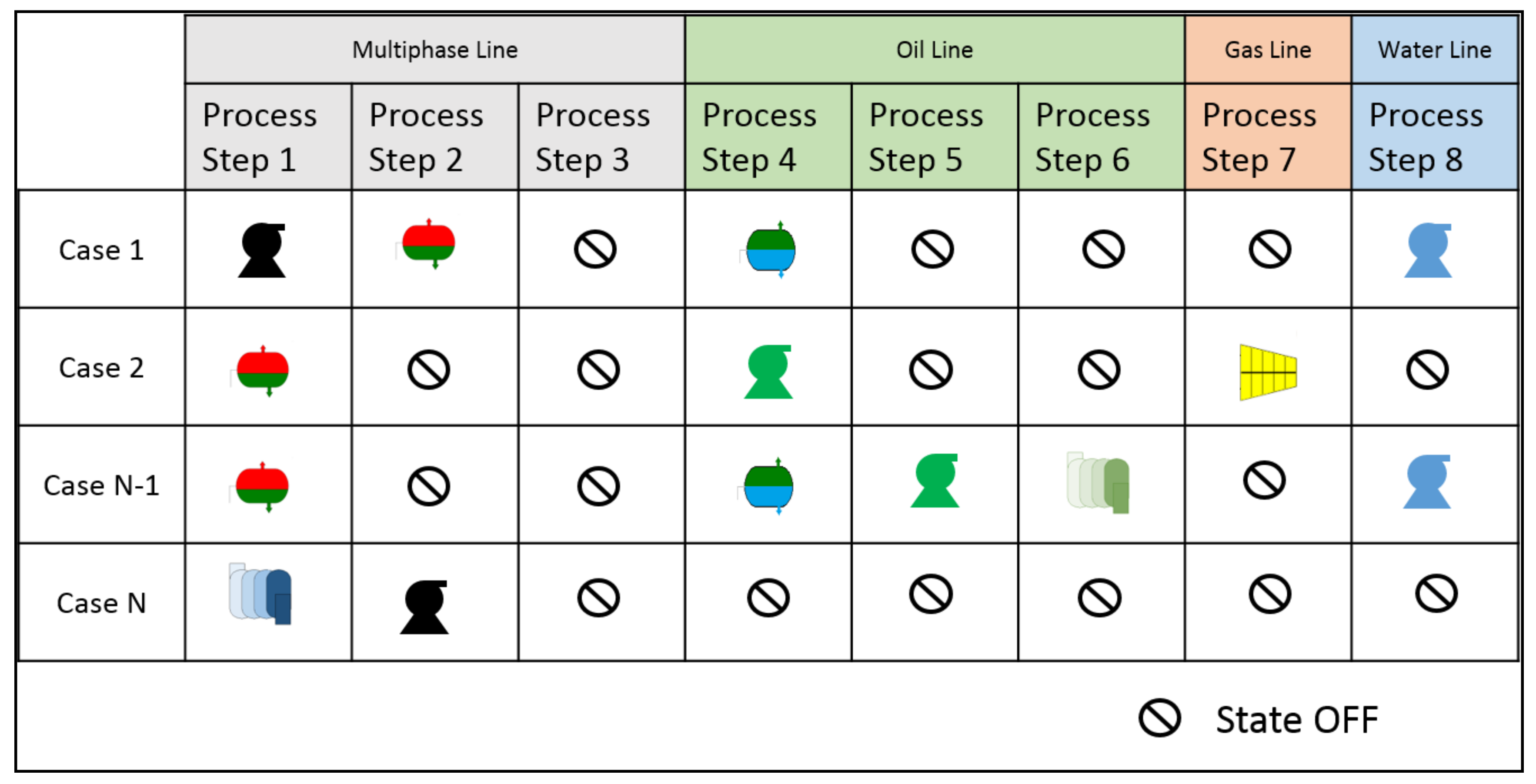
- The oil and gas branches are enabled after a gas–liquid separator.
- The water branch is enabled after an oil–water separator.
- The multiphase branch becomes disabled after a separator module.
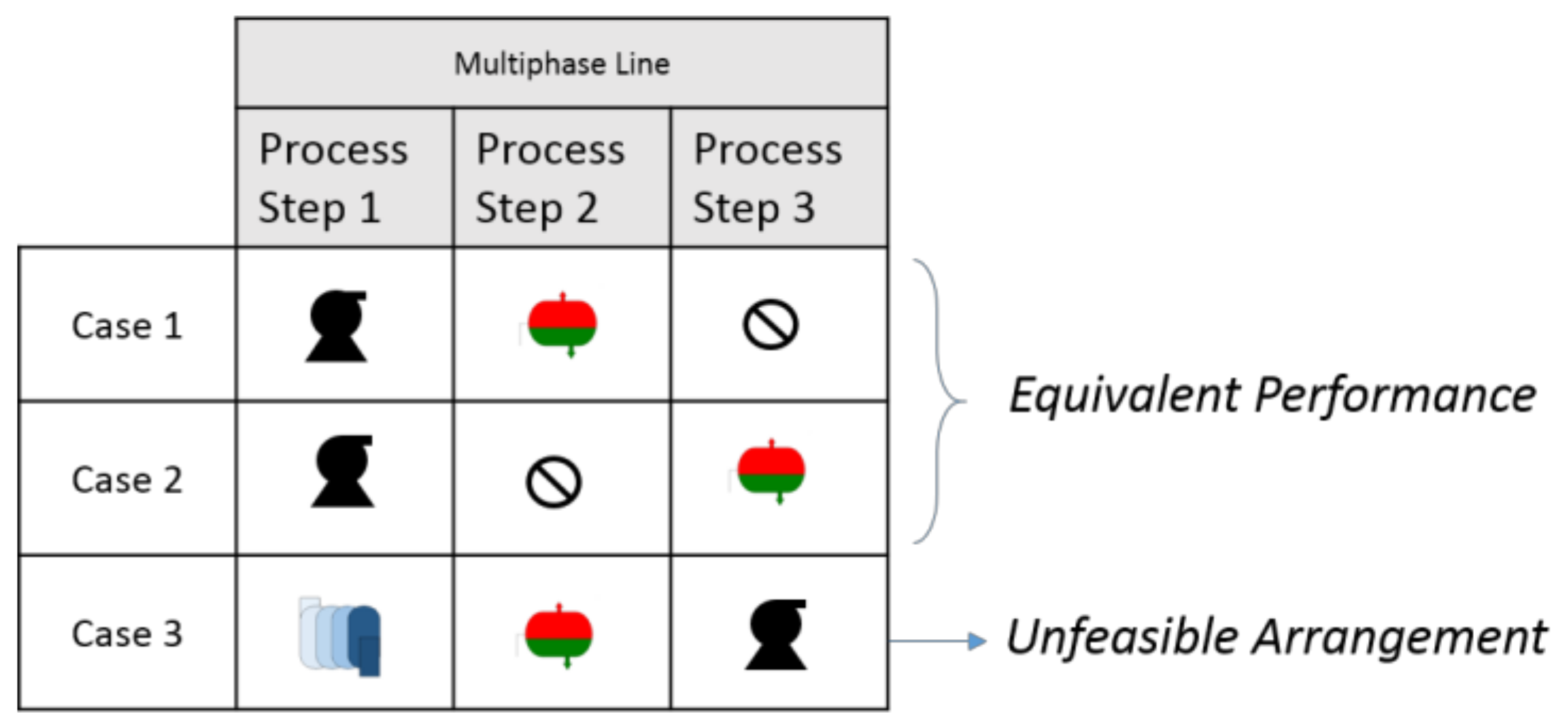
- The removal of duplicate cases (equivalent performance).
2.7. Evolutionary Algorithms
- Genetic Algorithms: A population of binary numbers or character strings evolve using a set of unitary and binary transformations and a selection process.
- Evolutionary Programs: A population of data structures evolve through a set of specific transformations and a selection process.
- Evolutionary Strategies: A population of real numbers is evolved to find the possible solutions of a numerical problem.
- Evolutionary Programming: The population is constituted by finite state machines that are subjected to unitary transformations.
- Differential Evolution: A direction-based search algorithm. It could be considered a real parameter-coded version of genetic algorithms, but the application and sequence of the variation operators differ with respect to the genetic algorithms and evolution strategies. The decision space is multidimensional [39].
- Genetic Programming: The population consists of programs that solve a specific problem. The objective is to evolve the population in order to find the best program that solves the problem under study.
2.7.1. Individuals Encoding and Initialization
- L = 1..
2.7.2. Population Initialization
2.7.3. Variation Operators
Crossover
- Parametric—Heuristic Crossover: Let be the chromosome corresponding to the lth position in the population during the rth generation: l = 1... and let and be two individuals selected from the population as parents: k ≠ l. The crossover produces the following offspring: and [21].where and are defined as in Equation (11). Parameter α must be a very small positive number compared to the order of magnitude associated with the gene’s values of each chromosome [21]. It can be also limited to a random or fixed number between 0 and 1; depending on the application [40,41], α can be also adaptive if required. For this application, α is randomly selected with uniform probability distribution between 0 and 1.
- Parametric—Arithmetic Crossover: Let be the chromosome corresponding to the lth position in the population during the rth generation: l = 1...Nind, and let and be two individuals selected from the population as parents: k ≠ l. The arithmetic crossover produces the following offspring: and [39].where and are defined as in Equation (11), and α is a random number with a uniform probability distribution between 0 and 1.
- Parametric Average/Intermediate Crossover: Let be the chromosome corresponding to the lth position in the population during the rth generation: l = 1...Nind, and let and be two individuals selected from the population as parents: k ≠ l. The average crossover produces the following offspringwhere and are defined as in Equation (11). This crossover generates only one child per operation.
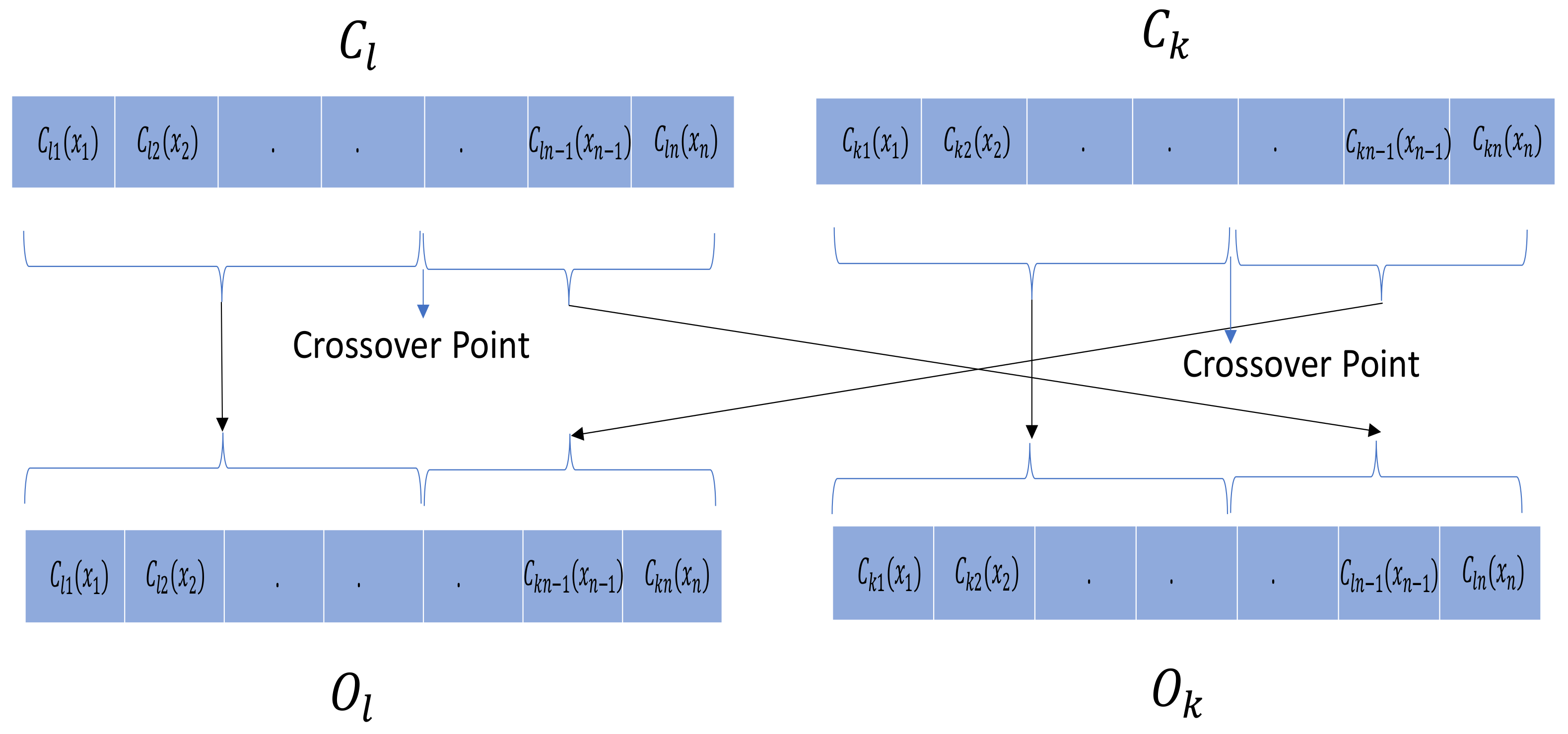
- Structural Segmented Crossover: It is a multipoint segmentation where the numbers of the points p = 1…n−1 are variables, randomly selected, given by a segmentation probability [38]. Let be the chromosome corresponding to the lth position in the population during the rth generation: l = 1...Nind, and let and be two individuals selected from the population as parents: k ≠ l. The segmented crossover is then performed as a combination of the parents at the crossover points, producing the offspring and . Figure 11 illustrates the p = 1 point segmented crossover.
- Structural Uniform Crossover: A uniform crossover selects the two parents and for the crossover at each generation r. It generates two offspring: and of n genes selected from both parents uniformly. Indexes l and k are positions in the r population, k ≠ l, with size Nind. Gene selection is driven by a random real number, between 0 and 1, with uniform probability distribution determining whether the first child selects the ith gen from the first or second parent [41]. The second child can be generated using the same process. Alternative solutions may also be applied to the second child, maintaining a uniform selection. For this specific application, the alternative solution applied to generate the second child was mirroring the parent genes not selected for the first child. Let and be two individuals selected from the population as parents: k ≠ l. The structural uniform crossover produces the offspring and ), where is produced using a random uniform probability distribution to decide the selection of the parent genes, and the second child ) may be generated using the same random process or, alternatively, using the opposite selection with respect to the first child as illustrated in Figure 12, where contains the gens not selected for . Then, ) = .
- Crossover Rate: The crossover rate or crossover probability defines the number of times a crossover operation occurs for chromosomes in one generation. The crossover rate is defined as a real number between 0 and 1. Different selection approaches can be applied depending on the application; they can be random, fixed, or adaptive. The authors of [42] presented a review on this topic including a dynamic approach. Adaptive and deterministic control methods for the crossover rate were also presented in [39]. For this application, the crossover rate was fixed set to 1 in order to maximize the number of solutions to be processed further within the EA without having the need to increase the population size prior to the crossing step. More details about the combined process within the proposed EA in this paper are documented in Section 2.7.10 and Section 3.
Mutation
- Boundary Mutation: This mutation operator replaces the genome with either a lower or upper bound randomly [39]. An alternative option, and the one used in this paper, is to replace the genome-containing values outside of the feasible domain boundaries with a random number uniformly distributed within the boundaries [L-U], where L is the lower boundary value and U is the upper boundary value. This is very useful for constrained optimization. Both approaches can be used for integer and float genes.
- Normal Mutation: A normal distribution disturbance is performed on one or more genes of a chromosome, where is the mean and the standard deviation. The normal distribution disturbance with can be written as [39]. The standard deviation can be fixed, random, or adaptive. The authors of [39] presented a review on normal mutation control parameters. Let be the chromosome corresponding to the lth position in the population during the rth generation: l = 1...Nind, where each gen is defined as per Equation (11).The mutant generated from using a normal mutation can be written as follows:
- Gradient Mutation: The gradient mutation is performed on one or more genes for a chromosome along a weighted gradient direction of the fitness function based on the algorithm originally proposed by [43] for nonlinear programming problems and adapted to be part of an evolutionary algorithm for linear systems identification in [21]. This mutation is oriented to maximize the fitness function f(x) using penalty functions of the type as constraints to penalize solutions out of the feasible domain, where x represents an individual of the population in the original algorithm. As the number of generations increases, the individuals/solutions with less fitness function value, as well as the nonfeasible solutions, will die gradually, and the fitness function is expected to reach the optimum or near-optimum value. A convergence analysis of this algorithm was presented in [43].To be consistent with the nomenclature defined for this application, as per Equation (11), let be an individual/chromosome corresponding to the lth position in the population, during the rth generation: l = 1..., where each gen is defined as per Equation (11). Let f() and g() be the fitness function and penalty function, respectively; then, the total gradient direction is defined as:Given the nature and complexity of this application, the gradient directions for f() and g() are calculated as finite differences of the fitness and penalty functions between the two consecutive generations and, therefore, defined as and respectively, where S is the total number of penalty functions or constraints associated with the problem, and are penalty function multipliers acting as the weights of the gradient direction, given bywhere will be a very small positive number.The mutant , generated from , along the weighted gradient direction , can be defined as:For the original algorithm presented in [43], is a step length of the Erlang distribution random number with declining means generated by a random number generator. For the Systems Identification application presented in [21], is a very small number compared to the order of magnitude associated with the individual gens adjusted to suit the specific applications. For the optimization problem presented in this paper, the gradient mutation was applied, tailoring a parameter control strategy to suit this problem statement. The application-specific details are described in the following subsections.
- Application Specific Gradient Mutation Penalization Functions:The following penalization functions were defined for this application:where m is the maximum number of feasible subsea gate box (SGB)/decentralized process module configuration cases, as defined in Equation (11).The above Equations (23) and (24) penalize solutions outside the feasible domain, having chromosome values greater than m or the negative.For this application and encoding, there is a risk of obtaining repeated solutions that have been evaluated and discarded; this can add unnecessary computational time within the EA, as well as additional IPM model simulation time, processing repeated solutions. In order to reduce this risk and maximize the exploration and diversity, all previous solutions that have been subjected to an evaluation in the previous (r−1)th generations are registered in an ancestors matrix: . Then, a third penalization function is defined as , whereSee more details regarding the ancestors matrix in Section 2.7.5.
- Application Specific Gradient Mutation Parameters Control: After the preliminary analysis and evaluation of gradient directions and penalization functions profiles, the need for defining the and parameters became apparent to control the order of magnitude of g( and the weighted gradient direction contributions with a different strategy, as originally defined in [21,43]. The parameters’ control for this application is dependent on the nature of the crossover operator used before mutation. Various scaling and normalization methods for the fitness and penalization functions were tested before to solve this issue without success; therefore, it was decided to define these parameters dynamically or statically, depending on the crossover operator being used. A heuristic crossover, for example, may generate solutions out of the feasible domain, and therefore, it may produce large values of the penalization functions g( during the first generation. Very small values of below 0.1 may produce large penalization multipliers and, therefore, large, weighted variations in the mutation, reducing the performance of the gradient contribution. For the rest of the crossover operators listed in this section, this does not occur. Therefore, when using a heuristic crossover operator before gradient mutation, selecting values of between 0.1 and 0.5 is appropriate for this application.On the other hand, when using the structural uniform crossover, no solutions outside the feasible domain are generated, and therefore, will be the only penalization function that can be activated. For this case, calculating is proposed based on the inverse average gradient direction of the fitness function for all individuals in the population at each generation as follows:where is the total number of individuals, as defined in Section 2.7.2. This allows controlling the magnitude order of the weighted gradient direction by controlling the amplitude of the penalization functions based on the average fitness function gradient direction, while keeping .Parameter performs better starting with small values when the gradient is large, increasing proportionally to the generation number to avoid a vanishing gradient contribution when the gradient decreases with the number of generations while approaching to an optimal or near-optimal solution. The following calculations are proposed to control , keeping :where corresponds to the generation number when the solution is expected to enter an attraction region where the optimum or a near-optimum is located. , where corresponds to the maximum number of generations given as one of the termination criteria in Section 2.7.9. is a parameter that can be fixed or adaptive. Based on all sensitivities performed, the majority of the qualifying cases reached the attraction region at the generation, on average. Therefore, was used for the associated cases, and the results are presented in Section 3.
- Mutation Rate: The mutation rate or mutation probability defines the number of times a mutation operation occurs for chromosomes in one generation. The mutation rate is defined as a real number between 0 and 1. Different selection approaches can be applied depending on the application; they can be random, fixed, or adaptive. The authors of [42] presented a review on this topic, including a dynamic approach. Adaptive and deterministic control methods for the mutation rate were also presented in [39]. For this application, two types of mutation rates were applied: one at the population level and one at the chromosome level. The one at the population level was tested for some cases with a mutation rate of 0.5, where the mutants were selected from the total, including only the offspring coming from the crossover process before the mutation. The mutation rate at the chromosome level is defined with two different random parameters, one determining the number of genes to be mutated and the second to determine the positions of the gens where the mutation will occur. The mutation rate can then be applied to the whole chromosome or to a part of it, depending on the parameter values. The parameters are chosen with a uniform probability distribution.
2.7.4. Filtration
2.7.5. Registration of New Individuals in the Ancestors Matrix
2.7.6. Evaluation
- Decoding of the chromosome structures into decentralized processing module configurations for the field.
- Reconfiguration of the superstructure integrated into the IPM with the decoded configuration from the EA.
- Run the IPM with the decoded configurations for the expected field life.
- Calculate the fitness function value based on the production potential obtained from the IPM, the development cost CAPEX, and the expected OPEX associated with the decoded configuration, as documented in Section 2.5.1.
- Transfer the fitness function value to the EA to continue the selection and ranking process, as documented in Section 2.7.7 and Section 2.7.8 as well as illustrated in Section 2.7.10.
2.7.7. Selection
- Conform the number of individuals or parents that will participate in the reproduction process.
- Control the population management, survivor’s selection, individual’s elimination, and/or replacement.
- Select the best individuals that satisfy the objectives to an optimization problem.
- Direct fitness rank-based selection: This method sorts the individuals from the highest to the lowest fitness values. This ranking is used to:
- -
- manage the population size by selecting the number of fittest individuals to continue to the next generation.
- -
- monitor and select the best individuals that satisfy the optimization objectives to control the termination criteria.
- -
- prioritize the set of parents that will be crossed based on their fitness values. This method may prematurely accelerate the convergence of the algorithm to a local attraction region.
- Direct fitness + gradient rank – based selection: This method sorts the individuals from the highest to the lowest fitness + gradient values. This is only used as an option to prioritize the set of parents that will be crossed based on their combined fitness + gradient values when the gradient mutation is used. This selection method was introduced for this specific application to avoid premature convergence of the algorithm to a suboptimal attraction region and keep the gradient energy, as well as continue exploring the solutions space as long as possible. This mechanism may deaccelerate the convergence speed but may increase the exploration capabilities and discovery of new solutions.
2.7.8. Replacement
2.7.9. Termination/Stop Criteria
2.7.10. Proposed Evolutionary Algorithm Flow Diagram
2.8. Business Case
3. Results
3.1. Field Concept Selection for the Business Case
3.2. Evolutionary Algorithm Performance
- 1.
- Fitness value of the best individual.
- 2.
- Inverse of the number of evaluations performed before finding the best individual.
- 3.
- Evaluation rate.
- 4.
- Survival rate.
- 5.
- Effectiveness.
- 6.
- Fitness Change (FC).
- 7.
- Inverse of the Total Number of Evaluations.
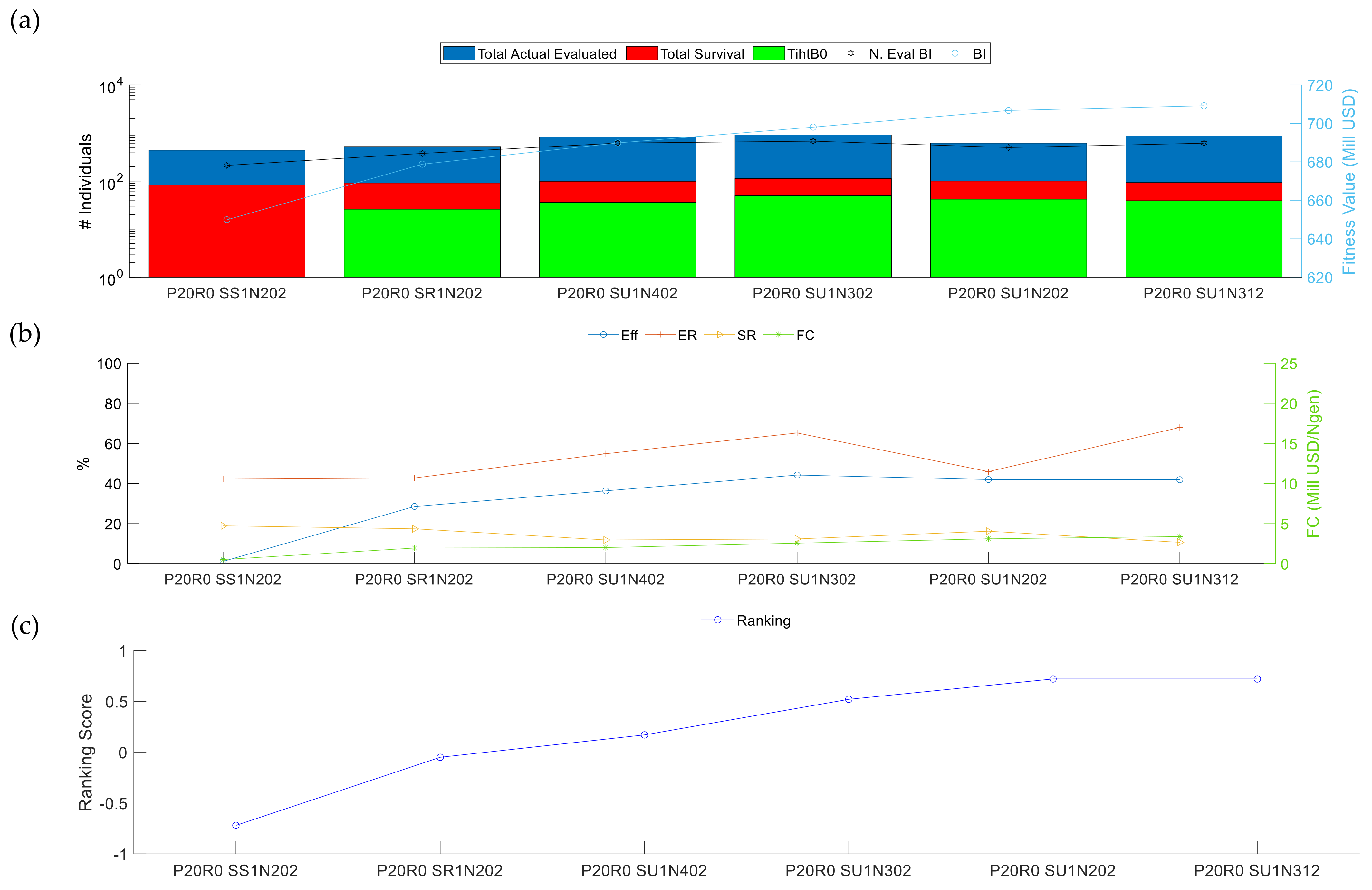
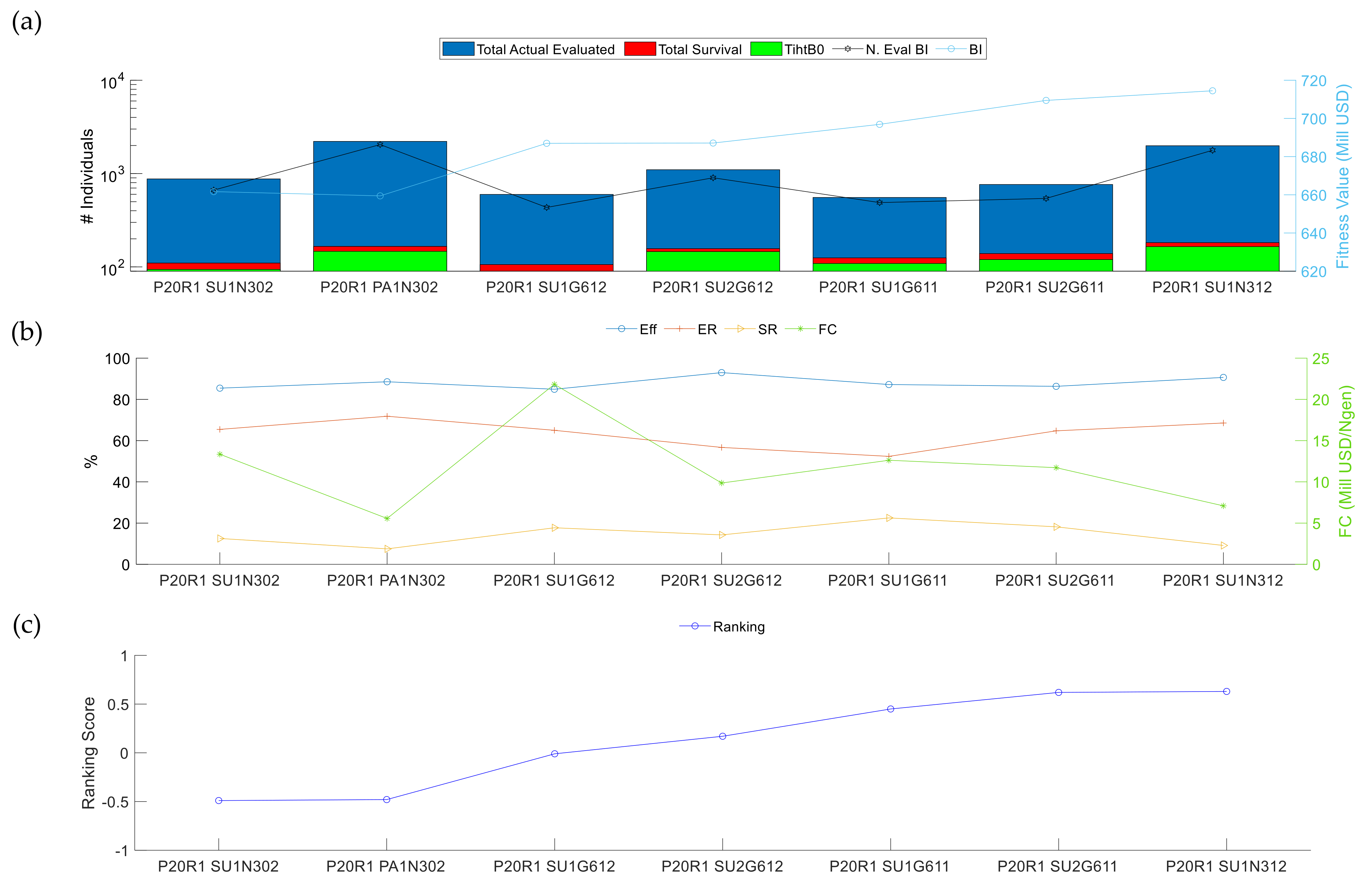
3.2.1. Analysis I: Performance of the Variation Operators
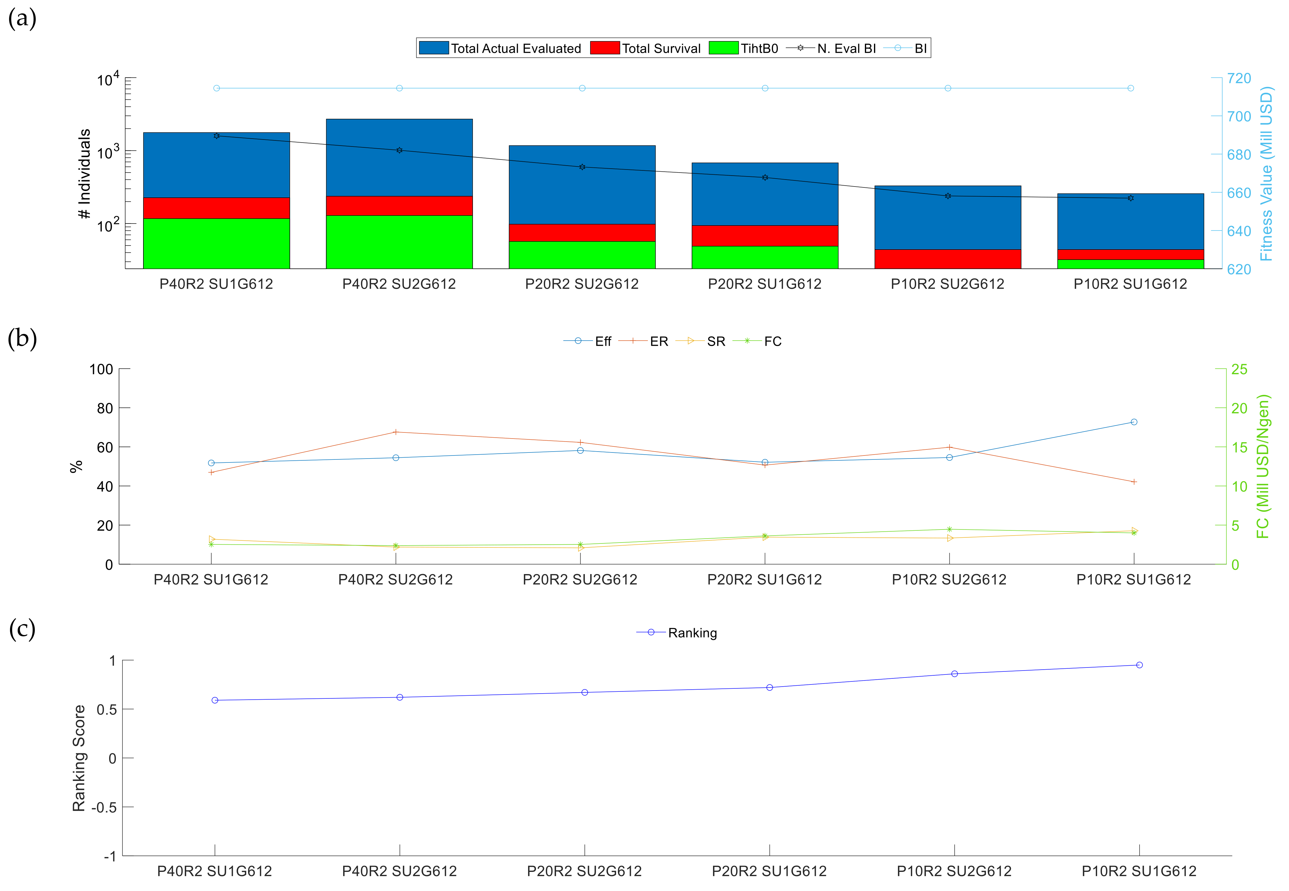
3.2.2. Analysis II: Initial Population Influences
3.2.3. Analysis III: Repeatability of the Results
4. Discussion
Future Works
- Selection mechanisms for population control, considering not only the best individuals but, also, a small number of the worst individuals, as proposed in [49]. Parent selection is performed randomly. Larger population sizes may be required, and therefore, a sensitivity analysis for the population size should be considered.
- Diversity-based adaptive EA [53] not only to prevent a premature convergence to the local optimum but also allow adaptive capabilities for dynamic problems.
5. Conclusions
Author Contributions
Funding
Institutional Review Board Statement
Informed Consent Statement
Data Availability Statement
Acknowledgments
Conflicts of Interest
References
- Diaz, M.J.C.; Stanko, M.; Sangesland, S. Exploring New Concepts in Subsea Field Architecture. In Proceedings of the Offshore Technology Conference, Houston, TX, USA, 30 April–3 May 2018; p. 14. [Google Scholar]
- Diaz, M.J.C.; Sangesland, S.; Stanko, M. The subsea gate box: And alternative subsea filed architecture. First SPE Nor. Mag. 2018, 2, 38. Available online: http://oslo.spe.org/thefirst (accessed on 18 January 2021).
- Diaz, M.; Sangesland, S.; Stanko, M. Enabling Flexible Subsea Architecture for Production Field with Large Heterogeneity among Wells; Internal Report; Norwegian University of Science and Technology: Trondheim, Norway, 2019; Unpublished. [Google Scholar]
- Irmann-Jacobsen, T.B.; Headridge, B. Ultimate Gas Recovery by Use of Full Field Simulations in Concept Selection Phase. In Proceedings of the Offshore Technology Conference-Asia, Kuala Lumpur, Malaysia, 25–28 March 2014; p. 11. [Google Scholar]
- Dianita, S.; Gandi, R.S. Full Field Integrated Modelling throughout Life-Cycle Phases of Field Development: A Subsea Processing Case Study. In Proceedings of theSPE/IATMI Asia Pacific Oil & Gas Conference and Exhibition, Nusa Dua, Bali, Indonesia, 20–22 October 2015; p. 15. [Google Scholar]
- Sauve, R.; Lindvig, T.; Stenhaug, M.; Holyfield, S. Integrated Field Development: Process and Productivity. In Proceedings of the Offshore Technology Conference, Houston, TX, USA, 6–9 May 2019; p. 19. [Google Scholar]
- Narayanan, K.; Cullick, A.S.; Matthew, B. Better Field Development Decisions from Multi-Scenario, Interdependent Reservoir, Well, and Facility Simulations. In Proceedings of the SPE Reservoir Simulation Symposium, Houston, TX, USA, 3–5 February 2003; p. 11. [Google Scholar]
- Smyth, J.; Rusin, P.; Garcia, J.J.; Cullick, S. Rapid Optimization of Development Scenarios for Multiple Exploration Prospects Using Integrated Asset Modeling. In Proceedings of the SPE Latin American and Caribbean Petroleum Engineering Conference, Lima, Peru, 1–3 December 2010; p. 21. [Google Scholar]
- Bouamra, R.; Vielliard, C.; Spilling, K.E.; Nilsen, F.P. Integrated Production Management Solution for Maximized Flow Assurance and Reservoir Recovery. In Proceedings of the OTC Brasil, Offshore Technology Conference, Rio de Janeiro, Brazil, 24–26 October 2017; p. 9. [Google Scholar]
- Saputelli, L.A.; Lujan, L.; Garibaldi, L.; Smyth, J.; Ungredda, A.; Rodriguez, J.; Cullick, S. How Integrated Field Studies Help Asset Teams Make Optimal Field Development Decisions. In Proceedings of the SPE Western Regional and Pacific Section AAPG Joint Meeting, Bakersfield, CA, USA, 29 March–4 April 2008; p. 16. [Google Scholar]
- Ogunyomi, B.A.; Jablonowski, C.J.; Lake, L.W. Field Development Optimization under Uncertainty: Screening-Models for Decision Making. In Proceedings of the SPE Annual Technical Conference and Exhibition, Denver, CO, USA, 30 October–2 November 2011; p. 11. [Google Scholar]
- Mikhin, A.; Salavatullin, K.; Kamartdinov, M. Main Aspects of the Integrated Asset Modeling and Gas Field Development Optimization under Surface Facilities Constraints. In Proceedings of the SPE Russian Petroleum Technology Conference, Moscow, Russia, 15–17 October 2018; p. 13. [Google Scholar]
- Rosa, V.R.; Camponogara, E.; Ferreira Filho, V.J.M. Design optimization of oilfield subsea infrastructures with manifold placement and pipeline layout. Comput. Chem. Eng. 2018, 108, 163–178. [Google Scholar] [CrossRef]
- Wang, Y.; Estefen, S.F.; Lourenço, M.I.; Hong, C. Optimal design and scheduling for offshore oil-field development. Comput. Chem. Eng. 2019, 123, 300–316. [Google Scholar] [CrossRef]
- Teixeira, A.F.; de Campos, M.; Barreto, F.P.; Stender, A.S.; Arraes, F.F.; Rosa, V.R. Model Based Production Optimization Applied to Offshore Fields. In Proceedings of the OTC Brasil, Offshore Technology Conference, Rio de Janeiro, Brazil, 29–31 October 2013; p. 11. [Google Scholar]
- Lin, P.; Bao, X.; Shu, Z.; Wang, X.; Liu, J. Test case generation based on adaptive genetic algorithm. In Proceedings of the 2012 International Conference on Quality, Reliability, Risk, Maintenance, and Safety Engineering, Chengdu, China, 15–18 June 2012. [Google Scholar]
- Khan, R.; Amjad, M. Automatic test case generation for unit software testing using genetic algorithm and mutation analysis. In Proceedings of the 2015 IEEE UP Section Conference on Electrical Computer and Electronics (UPCON), Allahabad, India, 4–6 December 2015. [Google Scholar]
- Mateen, A.; Nazir, M.; Afsar, S. Optimization of Test Case Generation using Genetic Algorithm (GA). Int. J. Comput. Appl. 2016, 151, 6–14. [Google Scholar] [CrossRef]
- Khan, R.; Amjad, M.; Srivastava, A.K. Optimization of Automatic Generated Test Cases for Path Testing Using Genetic Algorithm. In Proceedings of the 2016 Second International Conference on Computational Intelligence & Communication Technology (CICT), Ghaziabad, India, 12–13 February 2016. [Google Scholar]
- Khan, R.; Amjad, M.; Srivastava, A.K. Generation of automatic test cases with mutation analysis and hybrid genetic algorithm. In Proceedings of the 2017 3rd International Conference on Computational Intelligence & Communication Technology (CICT), Ghaziabad, India, 9–10 February 2017. [Google Scholar]
- Altamiranda, E.; Calderón, R.; Morles, E. An Evolutionary Algorithm for Linear System Identification. In Proceedings of the 6th WSEAS International Conference on Signal Processing, Robotics and Automation, Corfu Island, Greece, 16–17 February 2007. [Google Scholar]
- Radatz, H.; Schröder, M.; Becker, C.; Bramsiepe, C.; Schembecker, G. Selection of equipment modules for a flexible modular production plant by a multi-objective evolutionary algorithm. Comput. Chem. Eng. 2019, 123, 196–221. [Google Scholar] [CrossRef]
- Nagaiah, N.R.; Geiger, C.D. Application of evolutionary algorithms to optimize cooling channels. Int. J. Simul. Multidiscip. Des. Optim. 2019, 10, A4. [Google Scholar] [CrossRef]
- Healey, M.; Duff, S.; James, J. Optimization of a Subsea Design using an Evolutionary Algorithm. In Proceedings of the BHR 19th International Conference on Multiphase Production Technology, Cannes, France, 5–7 June 2019; p. 12. [Google Scholar]
- Castiñeira, P.P.; Baioco, J.S.; Couto, P.; Jacob, B.P. Optimal Positioning of Submarine Manifolds through Genetic Algorithms. In Proceedings of the 26th International Ocean and Polar Engineering Conference, Rhodes, Greece, 26 June–1 July 2016; International Society of Offshore and Polar Engineers: Rhodes, Greece; p. 5. [Google Scholar]
- Salam, D.D.; Gunardi, I.; Yasutra, A. Production Optimization Strategy Using Hybrid Genetic Algorithm. In Proceedings of the Abu Dhabi International Petroleum Exhibition and Conference, Abu Dhabi, UAE, 9–12 November 2015; p. 14. [Google Scholar]
- Motie, M.; Moein, P.; Moghadasi, R.; Hadipour, A. Separator Pressure Optimisation and Cost Evaluation of a Multistage Production Unit Using Genetic Algorithm. In Proceedings of the International Petroleum Technology Conference, Beijing, China, 26–28 March 2019; p. 14. [Google Scholar]
- Sambo, C.H.; Hematpour, H.; Danaei, S.; Herman, M.; Ghosh, D.P.; Abass, A.; Elraies, K.A. An Integrated Reservoir Modelling and Evolutionary Algorithm for Optimizing Field Development in a Mature Fractured Reservoir. In Proceedings of the Abu Dhabi International Petroleum Exhibition & Conference, Abu Dhabi, UAE, 7–10 November 2016; p. 10. [Google Scholar]
- Sayyafzadeh, M. A Self-Adaptive Surrogate-Assisted Evolutionary Algorithm for Well Placement Optimization Problems. In Proceedings of the SPE/IATMI Asia Pacific Oil & Gas Conference and Exhibition, Nusa Dua, Bali, Indonesia, 20–22 October 2015; p. 16. [Google Scholar]
- Henao, C.A. A Superstructure Modeling Framework for Process Synthesis Using Surrogate Models. In Chemical Engineering; University of Wisconsin-Madison: Madison, WI, USA, 2012; p. 210. [Google Scholar]
- Quaglia, A. An Integrated Business and Engineering Framework for Synthesis and Design of Processing Networks; Department of Chemical and Biochemical Engineering, Technical University of Denmark: Kongens Lyngby, Denmark, 2013; p. 240. [Google Scholar]
- Bertran, M.O.; Frauzem, R.; Zhang, L.; Gani, R. A Generic Methodology for Superstructure Optimization of Different Processing Networks. In Computer Aided Chemical Engineering; Kravanja, Z., Bogataj, M., Eds.; Elsevier: Amsterdam, The Netherlands, 2016; pp. 685–690. [Google Scholar]
- Khor, C.S.; Elkamel, A. Superstructure Optimization for Oil Refinery Design. Pet. Sci. Technol. 2010, 28, 1457–1465. [Google Scholar] [CrossRef]
- Krogstad, D. Superstructure Optimization of a Subsea Separation System; Department of Chemical Engineering, Norwegian University of Science and Technology: Trondheim, Norway, 2017. [Google Scholar]
- Rahmawati, S.D.; Whitson, C.H.; Foss, B.; Kuntadi, A. Integrated field operation and optimization. J. Pet. Sci. Eng. 2012, 81, 161–170. [Google Scholar] [CrossRef]
- ISO. Petroleum and natural gas industrues. Life-cycle costing. In Guidance on Application of Methodology and Calculations Methods; ISO: Geneva, Switzerland, 2001; p. 36. [Google Scholar]
- QUE$TOR 2019 Q3’s Help File; HIS Markit Inc.: Englewood, CO, USA, 2019.
- Aguilar, J.; Rivas, F. Computación Evolutiva. In Introducción a las Técnicas de Computación Inteligente; Universidad de Los Andes: Mérida, Venezuela, 2001. [Google Scholar]
- Yu, X.; Gen, M. Introduction to Evolutionary Algorithms; Decision Engineering; Springer: London, UK, 2010. [Google Scholar]
- Ackora-Prah, J.; Gyamerah, S.A.; Andam, P.S. A heuristic crossover for portfolio selection. Appl. Math. Sci. 2014, 8, 3215–3227. [Google Scholar] [CrossRef]
- Umbarkar, A.J.; Sheth, P.D. Crossover operators in genetic algorithms: A review. ICTACT J. Soft Comput. 2015, 6, 1083–1092. [Google Scholar]
- Hassanat, A.; Almohammadi, K.; Alkafaween, E.; Abunawas, E.; Hammouri, A.; Prasath, V.B.S. Choosing Mutation and Crossover Ratios for Genetic Algorithms—A Review with a New Dynamic Approach. Information 2019, 10, 390. [Google Scholar] [CrossRef]
- Jiafu, T.; Dingwei, W. A new genetic algorithm for nonlinear programming problems. In Proceedings of the 36th IEEE Conference on Decision and Control: San Diego, CA, USA, 12 December 1997. [Google Scholar]
- Tanaka, S.; Wang, Z.; Dehghani, K.; He, J.; Velusamy, B.; Wen, X.H. Large Scale Field Development Optimization Using High Performance Parallel Simulation and Cloud Computing Technology. In Proceedings of the SPE Annual Technical Conference and Exhibition, Dallas, TX, USA, 24–26 September 2018; p. 22. [Google Scholar]
- Gonzalez, D. Methodologies to Determine Cost-Effective Development Strategies for Offshore Fields during Early-Phase Studies Using Proxy Models and Optimization; Department of Geoscience and Petroleum, Faculty of Engineering, Norwegian University of Science and Technology: Trondheim, Norway, 2020. [Google Scholar]
- Stanko, M. Observations on and use of curves of current dimensionless potential versus recovery factor calculated from models of hydrocarbon production systems. J. Pet. Sci. Eng. 2021, 196, 108014. [Google Scholar] [CrossRef]
- Gobel, D.; Briers, J.; Chin, Y.M. Architecture and Implementation of an Optimization Decision Support System. In Proceedings of the International Petroleum Technology Conference, Beijing, China, 26–28 March 2013; p. 18. [Google Scholar]
- Cadei, L.; Rossi, G.; Montini, M.; Fier, P.; Milana, D.; Corneo, A.; Sophia, G. Machine Learning Advanced Algorithm to Enhance Production Optimization: An ANN Proxy Modelling Approach. In Proceedings of the International Petroleum Technology Conference, Dhahran, Kingdom of Saudi Arabia, 13–15 January 2020; p. 14. [Google Scholar]
- Jamróz, D.; Niedoba, T.; Pięta, P.; Surowiak, A. The Use of Neural Networks in Combination with Evolutionary Algorithms to Optimise the Copper Flotation Enrichment Process. Appl. Sci. 2020, 10, 3119. [Google Scholar] [CrossRef]
- Hickernell, F.J.; Yuan, Y. A simple multistart algorithm for global optimization. OR Trans. 1997, 1, 1–12. [Google Scholar]
- Martí, R.; Resende, M.G.C.; Ribeiro, C.C. Multi-start methods for combinatorial optimization. Eur. J. Oper. Res. 2013, 226, 1–8. [Google Scholar] [CrossRef]
- Tu, W.; Mayne, R. Studies of multi-start clustering for global optimization. Int. J. Numer. Methods Eng. 2002, 53, 2239–2252. [Google Scholar] [CrossRef]
- Gouvea, M.; Ribeiro, A. Diversity-Based Adaptive Evolutionary Algorithms. In New Achievements in Evolutionary Computation; Korosec, P., Ed.; Intech Slovenia: Ljubljana, Slovenia, 2010; p. 318. ISBN 978-953-307-053-7. [Google Scholar]
- Panahli, C.; Kleppe, J.; Bellout, M. Implementation of Particle Swarm Optimization Algorithm within FieldOpt Optimization Framework. Master’s Thesis, NTNU, Trondheim, Norway, 2017. Available online: http://hdl.handle.net/11250/2453090 (accessed on 10 January 2021).
- Onwunalu, J.; Durlofsky, L. Optimization of Field Development Using Particle Swarm Optimization and New Well Pattern Descriptions. Ph.D. Thesis, Stanford University, Stanford, CA, USA, 2010. Available online: http://purl.stanford.edu/tx862dq9251 (accessed on 10 January 2021).
- Windisch, A.; Wappler, S.; Wegner, J. Applying Particle Swarm Optimization to Software Testing. In Proceedings of the 9th Annual Conference on Genetic and Evolutionary Computation, London, UK, 7–11 July 2007. [Google Scholar]
- Adibifard, M.; Bashiri, G.; Roayaei, E.; Emad, M.A. Using Particle Swarm Optimization (PSO) Algorithm in Nonlinear Regression Well Test Analysis and Its Comparison with Levenberg-Marquardt Algorithm. Int. J. Appl. Metaheuristic Comput. 2016, 7, 1–23. [Google Scholar] [CrossRef]
- Suwannarongsri, S. Optimal Sizing of Hybrid Renewable Energy System via Flower Pollination Algorithm. WSEAS Trans. Environ. Dev. 2019, 15, 240–249. [Google Scholar]
- Yang, X.S. Flower Pollination Algorithm for Global Optimization. In Unconventional Computation and Natural Computation; Durand-Lose, J., Jonoska, N., Eds.; Springer: Berlin/Heidelberg, Germany, 2012; Volume 7445. [Google Scholar] [CrossRef]














| CAPEX | “Cover the relevant initial investment outlay Io, from discovery through appraisal, engineering, construction, and commissioning including modifications until normal operations are achieved.” |
| OPEX | “Cover the relevant costs over the lifetime of operating and maintaining the asset.” |
| Revenue impact | “Cover the relevant impact on the revenue stream from failures leading to production shutdowns, planned shutdowns, and penalties.” |
| Disposal/decommissioning | “Cover relevant costs of abandonment of the asset, if there will be a cost difference between alternatives evaluated.” |
| Date (dd/mm/yyyy) | Time Step in Resolve Simulations. Starting Time = Production Startup |
|---|---|
| # days | Cumulative number of days at each time step. This corresponds to the time step into the future (t) in Equation (1). Starting time = two years prior to production startup. |
| Base Case Qo (MSm3) | Cumulative Oil/Gas production at each time step for the base case scenario. The base case scenario is the original field without subsea processing or subsea gate boxes. |
| Base Case Qg (MSm3) | |
| Current Case Qo (MSm3) | Cumulative Oil/Gas production at each time step for the evaluated case. The evaluated case is one case among all possible SGB configurations. |
| Current Case Qg (MSm3) | |
| Extra Qo (m3) | Extra Oil/Gas production due to the modifications implemented in the evaluated case. This is the difference between the cumulative production of the evaluated case and the base case. |
| Extra Qg (Sm3) | |
| Energy (MWh) | Power consumption of pumps and compressors of the different SGB. |
| Extra Qo (USD) | Incomes of the extra Oil/Gas sells. Oil price (50 USD). |
| Extra Qg (USD) | |
| Energy (USD) | Expenditure for the energy consumption of the pumps and compressors of the different SGB (32 USD/MWH). |
| CAPEX (USD) | Capital expenditure according to the items in Table 3. The CAPEX is uniformly distributed during the two years prior to the first oil. |
| OPEX (USD) | Operational expenditure according to the items in Table 4. |
| Incomes (USD) | Sum of the incomes for the extra oil and gas. |
| Costs (USD) | Sum of the expenditure associated with the SGB. |
| (USD) | Net balance at the end of the time step. |
| FF (USD) | Equation (1) (discount rate = 10%). |
| Level | WBS ID | Project WBS Item Description |
| Level 0 | 0 | X Project Development |
| Level 1 | 1 | Facilities |
| Level 2 | 101 | Subsea |
| Level 3 | 10101 | SGB |
| Level 4 | 1010101 | Equipment |
| Level 5 | 101010101 | Multiphase Boosting |
| Level 5 | 101010102 | Oil Boosting |
| Level 5 | 101010103 | Water Boosting |
| Level 5 | 101010104 | Gas Boosting |
| Level 5 | 101010105 | Gas–Liquid Separation |
| Level 5 | 101010106 | Oil–Water Separation |
| Level 5 | 101010107 | Heater |
| Level 5 | 101010108 | Interconnection Module |
| Level 6 | 10101010801 | Structure |
| Level 6 | 10101010802 | Piles |
| Level 6 | 10101010803 | Manifold |
| Level 6 | 10101010804 | Subsea Distribution Unit |
| Level 6 | 10101010805 | Subsea Control Unit |
| Level 6 | 10101010806 | Internal Connectors |
| Level 5 | 101010109 | Equipment Freight |
| Level 3 | 10102 | Subsea Network |
| Level 4 | 1010201 | Equipment |
| Level 5 | 101020101 | Umbilical Connector Type 1 |
| Level 5 | 101020102 | Umbilical Connector Type 2 |
| Level 5 | 101020103 | Subsea Distribution Unit * |
| Level 5 | 101020104 | Equipment Freight |
| Level 4 | 1010202 | Material |
| Level 5 | 101020207 | PLET (Pipeline End Termination) |
| Level 5 | 101020208 | Flowline |
| Level 5 | 101020209 | Power cable Static-Umbilical |
| Level 5 | 101020210 | Power cable Dynamic Umbilical |
| Level 5 | 101020211 | Riser |
| Level 5 | 101020212 | Material Freight |
| Level 2 | 102 | Topside |
| Level 3 | 10201 | Power Generation |
| Level 3 | 10202 | Topside VSds (Variable Speed Drives) * |
| DSV For Inspection (days) | 0 |
| MSV For Repair (days) | f (Number of equipment) |
| Spares Costs (% CAPEX) | 1% |
| Reconditioning Cost (%Equipment without Freight) | 2% |
| Insurance OPEX (%CAPEX) | 0.5% |
| Item | Quantity | Unit Price | ||
|---|---|---|---|---|
| Pump station steel frame | F1(Tkw) | te | fix | USD |
| Pumps and motors | 1 | und | F2(Tkw) | USD |
| Subsea control module | 1 | und | fix | USD |
| Subsea step-down transformer | 0 | und | F3(Tkw) | USD |
| Subsea variable speed drive | 0 | und | F4(Tkw) | USD |
| Multiphase pumping process control module weight | F5(Tkw) | te | G1(F5(Tkw)) | USD |
| Design Parameters | Solution | ||
|---|---|---|---|
| Number of simultaneous SGB within the field | 3 SGB | ||
| Location of the SGB within the field | L1 | L3 | L4 |
| Number of process modules in a SGB | 2 | 2 | 1 |
| Process train sequence in a SGB | 1. Gas–Liquid separator 2. Liquid booster | 1. Gas–Liquid separator 2. Liquid booster | 1. Three-phase separator |
| Sensitivity Variable | Variable Value | Codification |
|---|---|---|
| Population size | Population size (P) given by XX and population group (R) given by Y | PXXRY |
| Crossover type | Parametric Average/Intermediate | PI |
| Structural Segmented | SS | |
| Parametric—Heuristic | PH | |
| Parametric—Arithmetic | PA | |
| Structural Uniform random | SR | |
| Structural Uniform | SU | |
| Parent Selection Method | Direct fitness rank-based | 1 |
| Direct fitness + gradient rank based | 2 | |
| Mutation type | Gradient +Boundary | G |
| Normal +Boundary | N | |
| Mutation Parameters Normal (µ, σ), Gradient (δ, β) | σ = 1, µ = 0 | 2 |
| σ = U (1–9), µ = 0 | 3 | |
| σ = U (1–5), µ = 0 | 4 | |
| Random: δ U (0.01–0.1); β U (0.1–1) | 5 | |
| Calculated δ Equation (26) β Equation (27) | 6 | |
| Random: δ = U (0.1–0.5); β Equation (27) | 7 | |
| Chromosome Mutation Rate | 100% | 0 |
| Random U (0–1) | 1 | |
| Population Mutation Rate | Mutation over children | 1 |
| Mutation over parents and children | 2 |
| Criteria | Weighting |
|---|---|
| Value of the best individual (BI) | 35% |
| Inverse of the number of evaluations performed before finding the best individual (1/N. Eval BI) | 25% |
| Effectiveness (Eff) | 25% |
| Fitness Change of the best individual (FC) | 5% |
| Survival rate (SR) | 4% |
| Evaluation rate (ER) | 3% |
| Inverse of Total Number of Evaluations (1/TE) | 3% |
| Total | 100% |
| Section/Case | Variable Parameters | Constant Parameters | Case Tag |
|---|---|---|---|
| Section 1 | Parametric crossover type | Boundary + Normal mutation type | P20R0 PI1N202 P20R0 PH1N201 P20R0 PH1N202 P20R0 PA1N202 P20R0 PA1N302 |
| Section 2 | Structural crossover type | Boundary + Normal mutation type | P20R0 SS1N202 P20R0 SR1N202 P20R0 SU1N402 P20R0 SU1N302 P20R0 SU1N202 P20R0 SU1N312 |
| Section 3 | Boundary + Gradient mutation type | Best Crossover from Section 1 and 2 | P20R0 PA1G611 P20R0 PH1G501 P20R0 PA1G612 P20R0 PH1G701 P20R0 PH2G701 P20R0 PH2G702 P20R0 SU1G612 P20R0 SU2G611 P20R0 SU2G612 P20R0 SU1G601 P20R0 SU1G611 |
| Codification | Description | Initial Best Individual (Mill USD) |
|---|---|---|
| P20R0 | Randomly generated population of 20 individuals | 641.45 |
| P20R1 | Randomly generated population of 20 individuals | 381.42 |
| P20R2 | Randomly generated population of 100 individuals and selecting the 20 best individuals for the evolution. | 638.46 |
| P20R3 | Randomly generated population of 100 individuals and selecting the 20 best individuals for the evolution | 573.17 |
| P20R4 | Randomly generated population of 100 individuals and selecting the best individual and 19 random individuals for the evolution | 573.17 |
| Fitness Value (Mill USD) | Genotype | Phenotype |
|---|---|---|
| 714.49 | [11,0,11,3,0,0] | |
| 714.20 | [11,0,11,1,0,0] |
| P20R0 SU2G612 | P20R0 SU1G612 | ||||
|---|---|---|---|---|---|
| µ | σ | µ | σ | ||
| Total actual evaluations (number of evaluations) | 16.1% | 971.80 | 187.02 | 819.00 | 59.79 |
| Total survivors (number of individuals) | 8.6% | 124.60 | 10.71 | 118.40 | 2.51 |
| TihtB0 (number of individuals) | 24.0% | 57.40 | 14.01 | 46.40 | 6.88 |
| Ngen (number of generations) | 16.1% | 25.20 | 4.87 | 23.60 | 2.41 |
| N. eval BI (number of evaluations) | 23.0% | 674.40 | 173.35 | 604.20 | 72.21 |
| BI (mill USD) | 0.3% | 711.56 | 4.36 | 708.13 | 7.21 |
Publisher’s Note: MDPI stays neutral with regard to jurisdictional claims in published maps and institutional affiliations. |
© 2021 by the authors. Licensee MDPI, Basel, Switzerland. This article is an open access article distributed under the terms and conditions of the Creative Commons Attribution (CC BY) license (http://creativecommons.org/licenses/by/4.0/).
Share and Cite
Díaz Arias, M.J.C.; dos Santos, A.M.; Altamiranda, E. Evolutionary Algorithm to Support Field Architecture Scenario Screening Automation and Optimization Using Decentralized Subsea Processing Modules. Processes 2021, 9, 184. https://doi.org/10.3390/pr9010184
Díaz Arias MJC, dos Santos AM, Altamiranda E. Evolutionary Algorithm to Support Field Architecture Scenario Screening Automation and Optimization Using Decentralized Subsea Processing Modules. Processes. 2021; 9(1):184. https://doi.org/10.3390/pr9010184
Chicago/Turabian StyleDíaz Arias, Mariana J. C., Allyne M. dos Santos, and Edmary Altamiranda. 2021. "Evolutionary Algorithm to Support Field Architecture Scenario Screening Automation and Optimization Using Decentralized Subsea Processing Modules" Processes 9, no. 1: 184. https://doi.org/10.3390/pr9010184
APA StyleDíaz Arias, M. J. C., dos Santos, A. M., & Altamiranda, E. (2021). Evolutionary Algorithm to Support Field Architecture Scenario Screening Automation and Optimization Using Decentralized Subsea Processing Modules. Processes, 9(1), 184. https://doi.org/10.3390/pr9010184


