Article

Multi-Objective Coordinated Optimal Allocation of DG and EVCSs Based on the V2G Mode

1
Department of Electrical Engineering and Automation, Fuzhou University, Fuzhou 350108, China
2
State Grid Quanzhou Power Supply Company, Quanzhou 362018, China
3
Department of Electrical and Computer Engineering, University of Michigan-Dearborn, Dearborn, MI 48128, USA
*
Author to whom correspondence should be addressed.
Processes 2021, 9(1), 18; https://doi.org/10.3390/pr9010018
Submission received: 4 December 2020 / Revised: 17 December 2020 / Accepted: 17 December 2020 / Published: 23 December 2020
(This article belongs to the Special Issue Multi-Period Optimization of Sustainable Energy Systems)

Abstract

:
With the vigorous promotion of new energy sources and the development of vehicle-to-grid (V2G) technology, the influence of the V2G mode should be considered in the joint optimal allocation of Distributed Generation (DG) and electric vehicle charging stations (EVCSs). The timing characteristics of the intermittent output of DG, conventional demand for load, and charging load of the electric vehicle (EV) are considered, as is its participation in grid interaction to examine the construction of typical scenarios and the EV cluster dispatching strategy. From the perspective of comprehensively planning the coordination of the distribution network, a DG-EVCSs bi-level joint planning model is established under the peak and valley price mechanism, with the sub-objectives of obtaining a comprehensive profit and high quality of voltage, curbing system load fluctuations, and satisfactorily charging the EV. An improved harmony particle swarm optimization algorithm is proposed to solve the bi-level model. The proposed method was tested on the IEEE-33 and the PG&E-69 (Pacific Gas and Electric Company) bus distribution systems, and the results show that the optimized configuration model that considers the V2G mode can improve the overall performance of the planning scheme, promote the use of clean energy, smoothen the load fluctuations of the system, and improve the quality of voltage and charging satisfaction of EV users.

1. Introduction

With increasing concerns about environmental pollution and the use of fossil fuels for energy, a growing number of applications are being proposed for distributed generation (DG) and electric vehicles (EV) [1,2,3,4]. The interconnection between large-scale distributed generation and electric vehicle charging stations (EVCSs) is expected to have an impact on the security and reliability of the distribution network. Therefore, the optimal allocation of DG and EVCSs has received extensive research attention in recent years.
The authors of [5] proposed a mixed-integer linear programming model to solve the problems of planning electrical distribution systems and allocating EVCSs, and proposed a robust optimal allocation scheme for the latter. An analytical expression was proposed in [6] for the evaluation of DG site selection schemes and involved transforming the random mixed-integer nonlinear programming problem into a deterministic integer problem to solve the DG programming problem. The work in [7] proposed an optimal allocation model of EVCSs, with the goal of minimizing the total annual cost of the charging system. In view of the complexity of the optimization model, a two-step equivalence method was proposed to transform the optimization model into a mixed-integer second-order cone programming problem through equivalence and precision relaxation. The capacity of the EVCSs was determined by considering the impact of traffic flow in [8], and the charging requirements of the infrastructure were integrated into the model to evaluate the economics of candidate schemes.
The above research originated in the separate planning of DG and EVCSs, without considering the coordination between them. The joint planning of DG and EVCSs is conducive to promoting the complementarity between the time-series characteristics of the output of DG and the charging load, to realize the on-site consumption of DG by EVs and improve the permeability of DG. Based on this, the authors of [9] designed a regional EVCSs system using wind power, photovoltaic, and energy storage systems. The minimum operational cost was taken as the objective function, and support vector regression was used to predict the on-grid price and the electricity market price. A two-stage stochastic programming model of EVCSs and photovoltaics was established in [10], and a generalized Benders decomposition algorithm was proposed to solve it. The work in [11] developed a grasshopper optimization algorithm to optimize the allocation of DG and EVCSs to reduce energy loss and improve the coefficient of voltage stability of the system.
With the development of vehicle-to-grid (V2G) technology, EVs will be connected to the grid as a controllable load and a mobile energy storage device and will participate in the dispatching of the power grid. The V2G mode will have an impact on power flow, network loss, the voltage quality. However, the research in [9,10,11] did not consider the influence of the V2G mode on distribution network planning, where this is important for engineering applications [12,13].
In this paper, a bi-level optimal allocation model for DG-EVCSs is established, considering the interaction between electric vehicles and the distribution network. The k-means++ clustering algorithm is used to establish typical daily scenarios of the wind-photovoltaic load. Based on the charging model for the electric vehicle, the bi-level optimal allocation model of DG-EVCSs is established by considering the peak and valley prices. At the upper planning level, an objective function is established based on comprehensive profit, voltage quality, the fluctuation in system load, and EV charging satisfaction. At the lower EV cluster scheduling level, the power flow is optimized in each typical scenario through the orderly management of the charging and discharging of the EV. The improved harmony particle swarm optimization (I-HSPSO) algorithm is proposed to solve the bi-level programming model. Finally, simulations based on the IEEE-33 bus distribution network and the PG and E-69bus distribution network are used to verify the effectiveness of the proposed model and its solution.

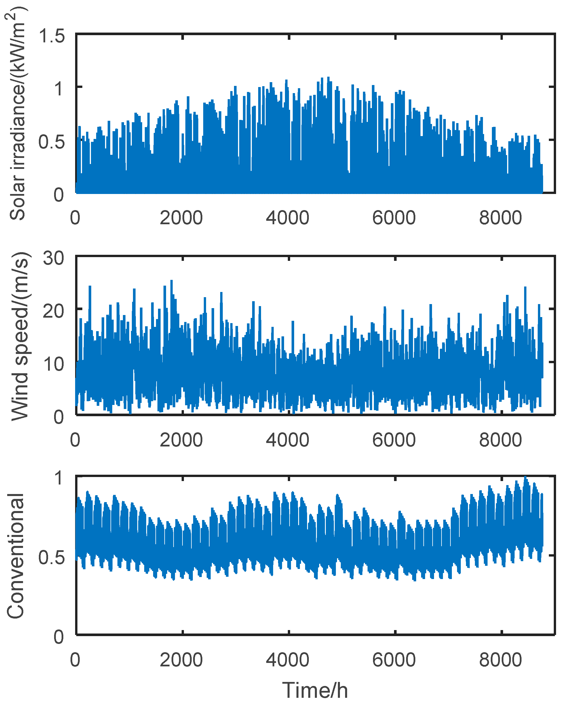
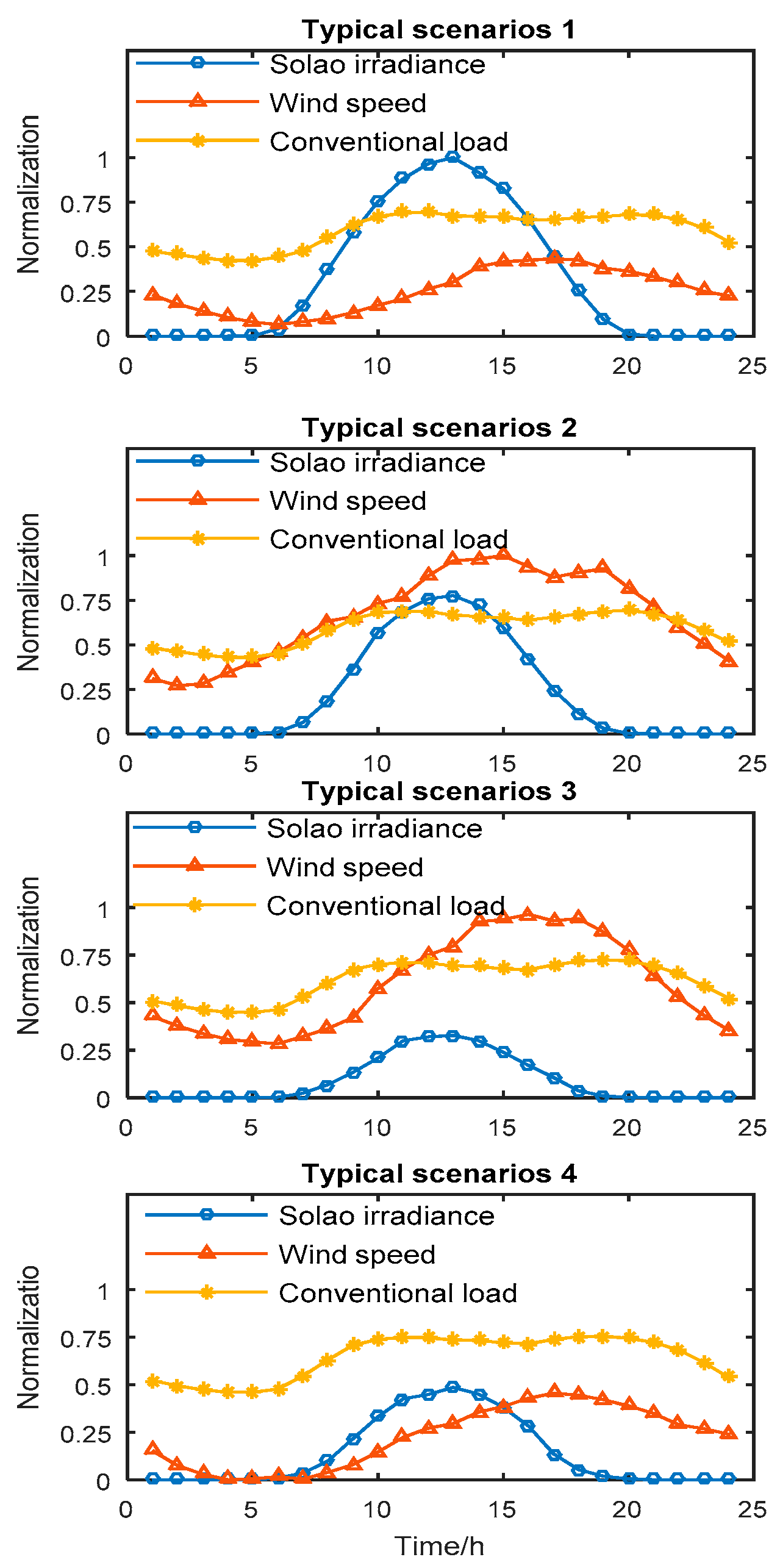
2. Construction of Typical Wind-Photovoltaic Load Scenarios

Distributed wind generation (DWG), photovoltaic generation (PVG), and load feature high uncertainty. The outputs of DWG and PVG are mainly affected by natural factors, such as wind speed and solar irradiance. The sampling period of wind speed is 15 s, but the period of photovoltaic and load data can only be 1 h, so all the data frequency is taken as 1 h. The wind speed, solar irradiance, and conventional demand for load for 8760 h a year in the planning area are presented in Figure 1.
It is clear from Figure 1 that the wind speed is high, and fluctuates significantly in spring and winter, and the solar irradiance in summer is clearly stronger than that in the other seasons. The conventional demand for load is higher in summer and winter. Therefore, it is necessary to consider the sequential temporal fluctuation in typical wind-photovoltaic load scenarios when planning the distribution network.
To avoid excessive calculations in the model, we use the k-means++ clustering algorithm [14] to optimize the scenario based on historical data for the planning area. Representative typical scenarios are thus extracted, and the validity of the results of clustering was verified based on the pseudo F-statistic (PFS) [15] to improve the computational efficiency of the model, while ensuring the distribution characteristics of the original scenarios.
The outputs of photovoltaic and wind power are closely related to wind speed and solar irradiance, respectively, and can be expressed as follows [16]:
P PV = { P P h h s h h s P P h > h s ,
where PPV indicates the output power of PVG, PP indicates the rated output of photovoltaic power, h and hs, respectively, indicate the actual solar irradiance and the rated solar irradiance.
P DW = { 0 0 v < v i   or   v o v P D v v i v s v i v i v < v s P D v s v < v o ,
where PDW indicates the output power of DWG, PD indicates the rated output of wind power, v indicates the actual wind speed, vi indicates the cut-in wind speed, v0 indicates the cut-off wind speed, and vs indicates the rated wind speed.

3. Charging and Discharging Model of EV in V2G Mode

There are four common types of EVs: buses, taxis, commercial cars, and private cars. According to the forecasts of vehicle ownership in 2020, there were a between 784,600 to 959,900 buses, 18,776 to 2,294,800 taxis, 8,022,000 to 9,805,200 business cars, and 74,687,400 to 91,284,600 private cars in China [17].Assuming that the ratio of the number of private electric cars to the total number of private cars is 10%, and the ratio of the number of each of other types of electric vehicles to the total number of respective vehicles in their categories is 15%, we can estimate that the ratio of number of electric buses, electric taxis, electric business cars, and electric private cars is 1: 2.4: 10.2: 63.5.
The charging mode of the EV is influenced by the initial state of charge (SOC), charging mode, charging power, and charging time. In addition, the demands for charging different types of EV are different. For example, the power consumption per 100 km of private electric vehicles is 20~30 kW·h and the battery capacity is 32 kW·h. The rechargeable period for private electric vehicles can be divided into a rest period at night and a work period during the day, namely 18:00~7:00 h and 8:00~17:00 h, respectively, and the charging power is 7 kW. The initial durations of charging for the two periods respectively satisfy the normal distributions N (9, 0.52) and N (19, 1.52). The modes and parameters of charging of the other types of electric vehicles are provided in [17].
In this paper, the Monte Carlo simulation was used to calculate the required duration of charging of the EV, which is expressed as Tf:
T f = ( S O C e S O C 0 ) η P e E e 60 ,
where SOCe indicates the percentage of batter capacity after charging, SOC0 indicates the percentage before charging, η indicates the charging efficiency, Pe indicates the charging power, and Ee indicates the battery capacity.
The EV charging limit time Tlim is determined according to the chargeable period of each type of EV, and the actual EV charging time is Tcd = min (Tf, Tlim).
With large-scale EVs in parallel in the grid, grouping electric vehicles into clusters and using cluster scheduling can help reduce the difficulty of system scheduling. For large-scale EVs, the daily charging mode has a certain rule of distribution. We thus developed a cluster scheduling strategy based on the EV charging model.
To participate in the V2G process, a number of complex factors need to be considered for buses, taxis, and official vehicles including operational needs and corporate willingness, while the participation of private cars depends on the willingness of their owners. Therefore, we used private electric cars as the object of scheduling of V2G to participate in EV cluster scheduling. The other three types of electric vehicles still used the plug-and-charge disorder charging mode.
The grid-connected time of the EV Tstar, required charging time Te, and off-grid time Tend are selected as the discriminant bases for EV cluster division, and the process consists of three steps:
(1)
According to the willingness of the users, EVs can be divided into two categories: owners willing to participate in V2G and owners unwilling to participate in V2G.
(2)
The required charging time of the EV Tf for the willing-to-participate group is calculated. If Tf is less than the charging time limit Tlim, the given of EV is classed in the same cluster as the unwilling-to-participate group owing to its lack of V2G capabilities.
(3)
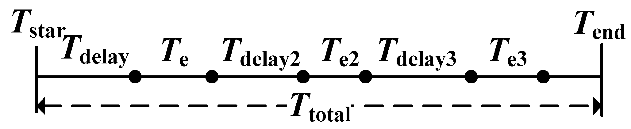
We cluster EVs the owners of which were willing and able to participate in V2G according to Tstar, Te, and Tend. For example, when an EV was connected to the grid from 18:00~19:00 h, the charging time was three to four h, and the off-grid time was 7:00 h the next day. Such EVs were placed in the same cluster.
The total grid-connection time of the EV is set to Ttotal. To avoid the loss of battery owning to frequent charging and discharging, the maximum daily discharge frequency of EVs under the V2G mode was set to one. The discharge operation was not allowed until the initial charging of the EVs was complete, and the discharge was terminated before reaching the maximum allowable discharge level. Then, secondary charging was performed according to the scheduling instructions until charging was terminated. The charging and discharging time distributions of the EV are shown in Figure 2. Tdelay indicates the first delay in charging, Tdelay2 indicates the delay, Tdelay3 indicates the second delay, Te and Te2, respectively, indicate the charging and discharging times, Te3 indicates the second charging time, and Tend indicates the off-grid time of the EV.
For different clusters of the EV, the EV cluster scheduling strategy can be formulated by setting Tdelay, Tdelay2, Tdelay3, Te2, and Te3.

4. Bi-Level Optimization Model

The bi-level model is a hierarchical system optimization model, in which the upper and low levels have their own mathematical models. We use programming as the upper level and EV cluster scheduling as the lower level to build a multi-objective optimization model of DG and EV charging stations.

4.1. Mathematical Model of the Upper Level

The decision variables of the upper level planning problem are the locations and capacity of DG and EVCSs. A multi-objective optimization model is established with the objective of obtaining the maximum overall profit, optimal voltage quality, minimum fluctuations in system load, and the maximum charging satisfaction of the EV.
Comprehensive profit F1
max F 1 = C SS + C B C inv C OM C loss + C env ,
where CSS indicates the profit of the distribution company, CB indicates the subsidy from the government for renewable energy sources, Cinv indicates the investment on intermittent DG and EVCSs, COM indicates the maintenance fee for DG and EVCSs, Closs indicates the cost of network loss, and Cenv indicates the environmental profit due to the use of clean energy.
C SS = l = 1 k s T l t = 1 24 ( c o ( t ) P l , t , L c i ( t ) ( P l , t , L P l , t , DWG P l , t , PV + P l , t , EV c P l , t , EV d ) + ( c e ( t ) P l , t , EV c c f ( t ) P l , t , EV d c b P l , t , EV d ) ) ,
where co(t), ci(t), ce(t), and cf(t), respectively, indicate the sale price of electricity charged by the distribution company, the price it pays, the unit charging cost of EVCSs, and the discharge compensation coefficient at time t. ks indicates the number of typical scenarios, Tl indicates the probability for lth typical scenario obtaining, Pl,t,L, Pl,t,DWG and Pl,t,PV, respectively, indicate the load demand, output power of DWG, and output power of PV at time t, Pcl,t,EV and Pdl,t,EV, respectively, indicate the charging and discharging powers of the EV at time t, and cb indicates the compensation coefficient of battery loss.
C B = l = 1 k s T l t = 1 24 ( c b , DWG P l , t , DWG + c b , PV P l , t , PV ) ,
where cb,DWG and cb,PV respectively indicate unit subsidies from the government for DWG and PV.
C inv = ( j = 1 n DWG c t 1 P j , DWG + j = 1 n PV c t 2 P j , PV + j = 1 n EV ( c g + c t 3 P j , E V ) ) r ( 1 + r ) n 1 ( 1 + r ) n 1 1 ,
where nDWG, nPV, and nEV, respectively, indicate the number of candidate nodes for DWG, PVG, and EVCSs, Pj,DWG, Pj,PV, and Pj,EV, respectively, indicate the capacity for DWG, PVG, and EVCSs at node j, ct1, ct2, and ct3, respectively, indicate the costs of construction of unit capacity of the DWG, PVG, and EVCSs, cg indicates the fixed investment cost of EVCSs, r indicates the discount rate, and n1 indicates the service life of the equipment.
C OM = l = 1 k s T l t = 1 24 ( c om 1 P l , t , DWG + c om 2 P l , t , PV ) + j = 1 n EV ( c om 3 P j , EV ) ,
where com1 and com2 respectively indicate the unit maintenance fees for DWG and PVG, and com3 indicates the amortized unit maintenance fee for EVCSs.
C loss = l = 1 k s T l t = 1 24 c o P l , t , loss ,
where Pl,t,loss indicates the system loss at time t.
C env = l = 1 k s T l t = 1 24 ( ( P l , t , DWG + P l , t , PV ) s = 1 N env x s ( a s + b s ) + P l , t , EV e EV c co 2 Δ ) ,
where Cenv indicates the social welfare of renewable energy sources and reduced emissions due to EVs, Nenv indicates the types of pollutant gases, xs, as, and bs, respectively, indicate the emission levels of the sth kind of pollution gas, eEV indicates the energy consumed by an EV over 100 miles, cco2 indicates the CO2 trading tax fee in the international market, and Δ indicates the difference between EVs and conventional vehicles.
Voltage quality F2
max F 2 = l = 1 k s T l 365 24 i = 1 Z t = 1 24 ( U i ( t ) U i min ) ( U i r U i min ) ( U i max U i ( t ) ) | P i ( t ) | ( U i max U i r ) j = 1 Z | P j ( t ) | ,
where Z indicates the number of system nodes, Uir indicates the voltage rating at node i, Pi(t) indicates the injected active power at the i-th node at time t, Ui(t) indicates the voltage of the i-th node at time t, and Uimax and Uimin, respectively, indicate the upper and lower limits of voltage at the i-th node.
System load fluctuation F3
min F 3 = l = 1 k s T l 365 t = 1 24 ( P l , t , e P l , ave ) 2 24 ,
P l , t , e = P l , t , L + P l , t , EV P l , t , DG ,
where Pl,t,e indicates the equivalent load of the system at time t under scenario l, and Pl,ave indicates its average load under scenario l.
Charging satisfaction of EVF4
max F 4 = l = 1 k s T l 365 ( α 1 c l , wcd + α 2 1 c l , cb ) ,
where cl,wcd indicates the completion of charging of the EV cluster under scenario l, cl,cb indicates the unit charging cost of the EV cluster under scenario l, and α1 and α2 respectively indicate the weight of complete charging and unit charging cost satisfaction.
The above four objective functions are normalized as follows:
f i * = { F i / F i max i = 1 , 2 , 4 F i min / F i i = 3 ,
where f i * indicates the normalized value of the sub-objective function Fi, and F i max and F i min indicate the optimal values of the subobjective function in the optimization process.
The multiple objective functions were aggregated into comprehensive evaluation indices maxfU by linear weighting:
max f U = i = 1 4 w i f i * ,
where wi indicates the weight of the sub-objective function f i * . In this paper, the weight coefficient of the sub-objective function is determined based on the Analytic Hierarchy Process (AHP) [18].
The constraints on the upper-level optimization model are:
P DG i P DG i max ,
P DG i P DG max ,
P EV i min P EV i P EV i max ,
where PDGi indicates the installed capacity of DG at node i, P DG i max indicates the installed capacity limit of DG at node i, P DG max indicates the limit of the total installed capacity of DG in the system, PEVi indicates the installed capacity of the EVCSs at node i, and P EV i max and P EV i min , respectively, indicate the upper and lower limits of the installed capacity of the EVCSs at node i.

4.2. Mathematical Model of the Lower Level

Based on DG and the EVCSs planning scheme determined by the upper level, the lower layer formulates the cluster scheduling strategy for the EVs, and manages their charging and discharging in an orderly manner to achieves the optimal overall operation of the system. The objective function of the lower level can be expressed as:
max f L = w 1 f l , 1 * + w 2 f l , 2 * + w 3 f l , 3 * + w 4 f l , 4 * ,
F l , 1 = C l , S + C l , B C l , OM C l , loss + C l , env ,
F l , 2 = 1 24 i = 1 Z t = 1 24 ( U i ( t ) U i min ) ( U i r U i min ) ( U i max U i ( t ) ) | P i ( t ) | ( U i max U i r ) j = 1 Z | P j ( t ) | ,
F l , 3 = t = 1 24 ( P l , t , e P l , ave ) 2 / 24 ,
F l , 4 = α 1 c l , wcd + α 2 / c l , cb ,
where f l , 1 * , f l , 2 * , f l , 3 * , and f l , 4 * , respectively, indicate the normalized values of the comprehensive profit index Fl,1, the voltage quality index Fl,2, the system load fluctuation index Fl,3, and the EV charging satisfaction index Fl,4.
The constraints on the lower-level optimization model are:
{ P i U i j i U j ( G i j cos θ i j + B i j sin θ i j ) = 0 Q i U i j i U j ( G i j sin θ i j B i j cos θ i j ) = 0 ,
U i min U i U i max ,
I i j I i j max ,
S O C min S O C S O C max ,
S O C end S O C ex ,
T delay + T e + T delay 2 + T e 2 + T delay 3 + T e 3 T total ,
where Pi and Qi, respectively, indicate the injected active power and the injected reactive power at the i-th node, Ui and Uj, respectively, indicate the voltage at the i-th node and the j-th node, Gij, and Bij, respectively, indicate the conductance and susceptance between the i-th and the j-th nodes, θij indicates the difference in voltage angle between the i-th and the j-th nodes; Uimax and Uimin, respectively, indicate the upper and lower limits of voltage at the i-th node, Iij indicates the actual current through the branch ij, Imaxij indicates the maximum current through the branch ij, SOCmax and SOCmin, respectively, indicate the upper and lower limits of battery capacity, SOCex indicates the expected value of SOC at the end of charging, and SOCend indicates the actual value of SOC when the EV is off the grid.

5. Optimal Solution of the Proposed Bi-Level Model

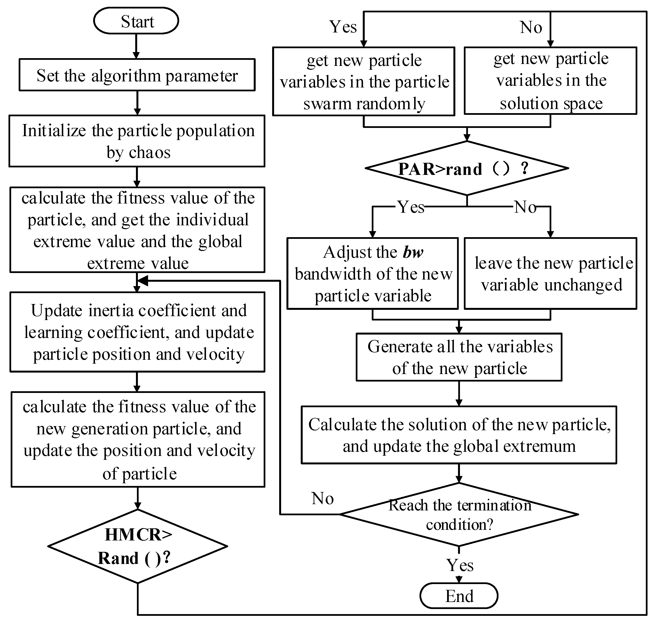
5.1. Improved Harmonic Particle Swarm Optimization

Particle swarm optimization (PSO) simulates the principle of foraging by a swarm of birds and has the advantages of simple calculation and strong directionality [19]. However, the global search ability of the PSO algorithm is poor, and it can easily fall into the local optimum in the later stage. Therefore, this paper optimizes the PSO algorithm to improve its convergence-related.
Chaos is a kind of irregular state of motion with strong nonlinearity. The initialization of the particle swarm by introducing a chaos variable is beneficial for generating a more uniform initial particle swarm. To improve the ergodic property of the initial particle in the search space, chaotic initialization is carried out on the particle swarm:
x i , j = x j min + ( x j max x j min ) χ i , j ,
χ i , j + 1 = λ χ i , j ( 1 χ i , j ) ,
where xi,j indicates the j-dimension value of particle i, x j max and x j min , respectively, indicate the upper and lower limits, xi,j indicates the sequences of chaotic variables generated by the logistic model, the chaotic parameters λ is set to four.
Of the PSO parameters, the optimization of the inertial coefficient ω is beneficial for balancing the global and the local search capabilities of the PSO algorithm. The optimization is expressed as follows:
ω = ω max ω min 2 cos ( π t / T PSO ) + ω max + ω min 2 ,
where ωmax and ωmin, respectively, indicate the upper and lower limits of the inertial coefficient, t indicates the number of iterations at the given time, and TPSO indicates the maximum number of iterations.
The learning coefficients c1 and c2, respectively, reflect the self-cognition ability and social cognition ability of the particle. The optimization of the learning coefficient can strengthen the self-learning ability of the particle swarm in the initial stage to avoid falling into the local optimum, and improves its ability to learn from the optimal solution for the group to find the optimal solution:
{ c 1 = c 1 max + t ( c 1 min c 1 max ) / T PSO c 2 = c 2 min + t ( c 2 max c 2 min ) / T PSO ,
The harmony search (HS) principle is introduced in this paper. Although the directivity of the HS algorithm is not strong, it has the characteristic of expanding the search range in the later stage of execution. Therefore, a novel combination harmony principle of the HS algorithm is introduced to the particle optimization process of the PSO algorithm, and the optimal particle is found within the search space with a certain probability in each iteration to improve the performance of the algorithm in terms of global search.
The flow of calculation of the improved harmony search particle swarm optimization (I-HSPSO) is shown in Figure 3.

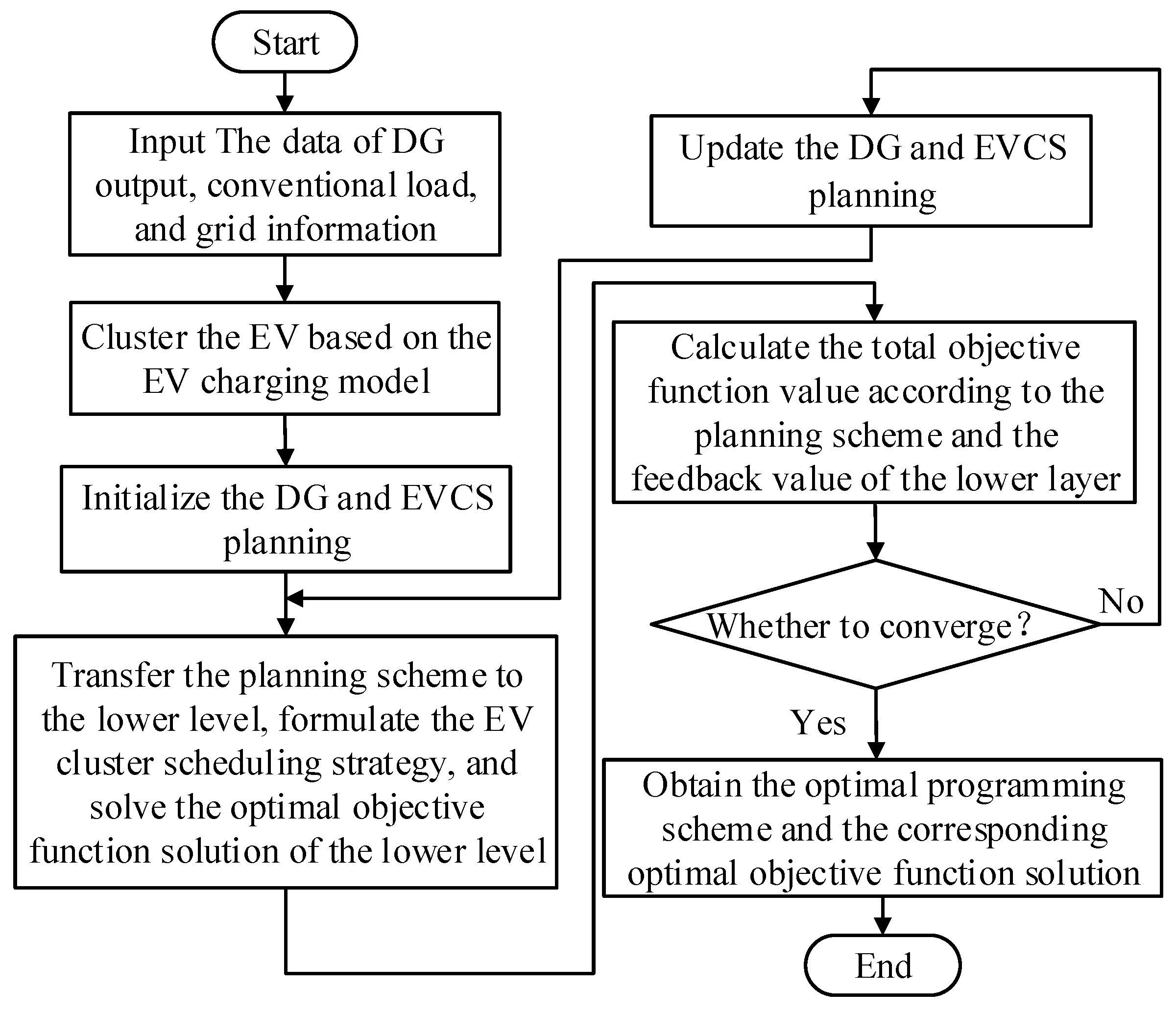
5.2. Flowchart of Bi-Level Programming Model

The flow of the bi-level optimization model established in this paper is shown in Figure 4.
The bi-level optimization model is solved based on the I-HSPSO algorithm, where the upper level makes decisions on site selection and capacity determination of DG and the EVCSs, and the lower level formulates the scheduling strategy for each EV cluster. At the lower level, the charging and discharging of the EV are managed in an orderly manner to optimize power flow in each typical scenario, and the optimal solution maxfL is fed back to the upper level, where the optimal solution maxfU of the overall objective function is calculated according to the scheme and maxfL to obtain the optimal scheme for DG and the EVCSs.

6. Case Study

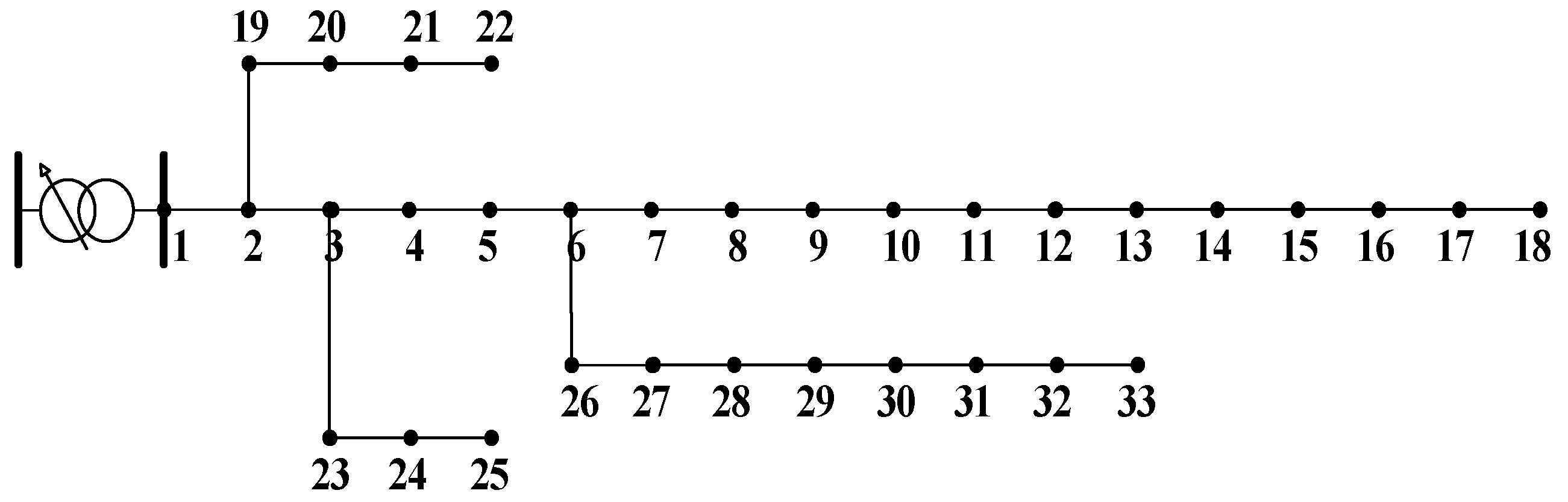
6.1. Parameters of the IEEE-33 Bus Test System

In this paper, the IEEE-33 bus test system was used for a simulation analysis of the proposed DG-EVCSs planning, and is shown in Figure 5. The system parameters are described in [20].
It was assumed that the number of EVs in the planning area was 900, and that they were evenly distributed among sub-stations. According to the ratio of each type of EV, the number of private electric vehicles was 740. It was assumed that the ratio of EV users willing to participate in the V2G mode was 90%, efficiency of charging and discharging efficiency was 90%, charging and discharging power was 7 kW, and the compensation coefficient of battery loss was 0.854 CNY/kWh. The peak and valley prices were used to calculate the prices of electricity for the distribution network and the EVCSs, and the values are shown in Table 1.
For the IEEE-33 bus test system, the DWG candidate nodes were nodes 13, 23, and 31, the PV candidate nodes were nodes 7, 21, and 28, and the EVCSs candidate nodes were nodes 4, 8, 14, 20, and 29. The weights of the completion of charging and unit charging cost satisfaction α1 and α2 were 0.4 and 0.6, respectively. The weight coefficients of the sub-objective function w1, w2, w3, and w4 are 0.375, 0.125, 0.125, and 0.375, respectively. The rated power for DG was 100 kW, the cut-in wind speed, rated wind speed, and cut-off wind speed of DWG were 13.5 m/s, 3 m/s, and 20 m/s, respectively, and the rated solar irradiance of PV was 1 kW/m2. The government subsidy cb,DWG was 0.1 CNY/kWh and cb,PV was 0.36 CNY/kWh. The capacity construction costs ct1, ct2, and ct3 were 5381 CNY/kWh, 4735 CNY/kWh, and 6000 CNY/kWh, respectively. The fixed investment cost of the EVCSs is 3,000,000 CNY. The service life of the equipment n1 was 20 years, and the discount rate was 8%. The unit maintenance fees were com1 = 0.0296 CNY/kWh and com2 = 0.0096 CNY/kWh, and the amortized unit maintenance fee for the EVCSs was 100 CNY/kWh. The energy consumed by an EV over 100 miles was 21.5 kWh, the CO2 trading tax fee in the international market was 80 CNY/ton, and the difference between the EVs and conventional vehicles over 100 miles Δ was 7 kg. The cost parameters of environmental pollution are shown in Table 2.
The four typical scenarios of wind speed, solar irradiance, and conventional demand for load, obtained based on the maximum principle of the pseudo F-statistic (PFS), are shown in Figure 6. Based on the uncertainty of wind power and light, four typical scenarios constructed in this paper represent the fluctuations of wind speed and light throughout the year.

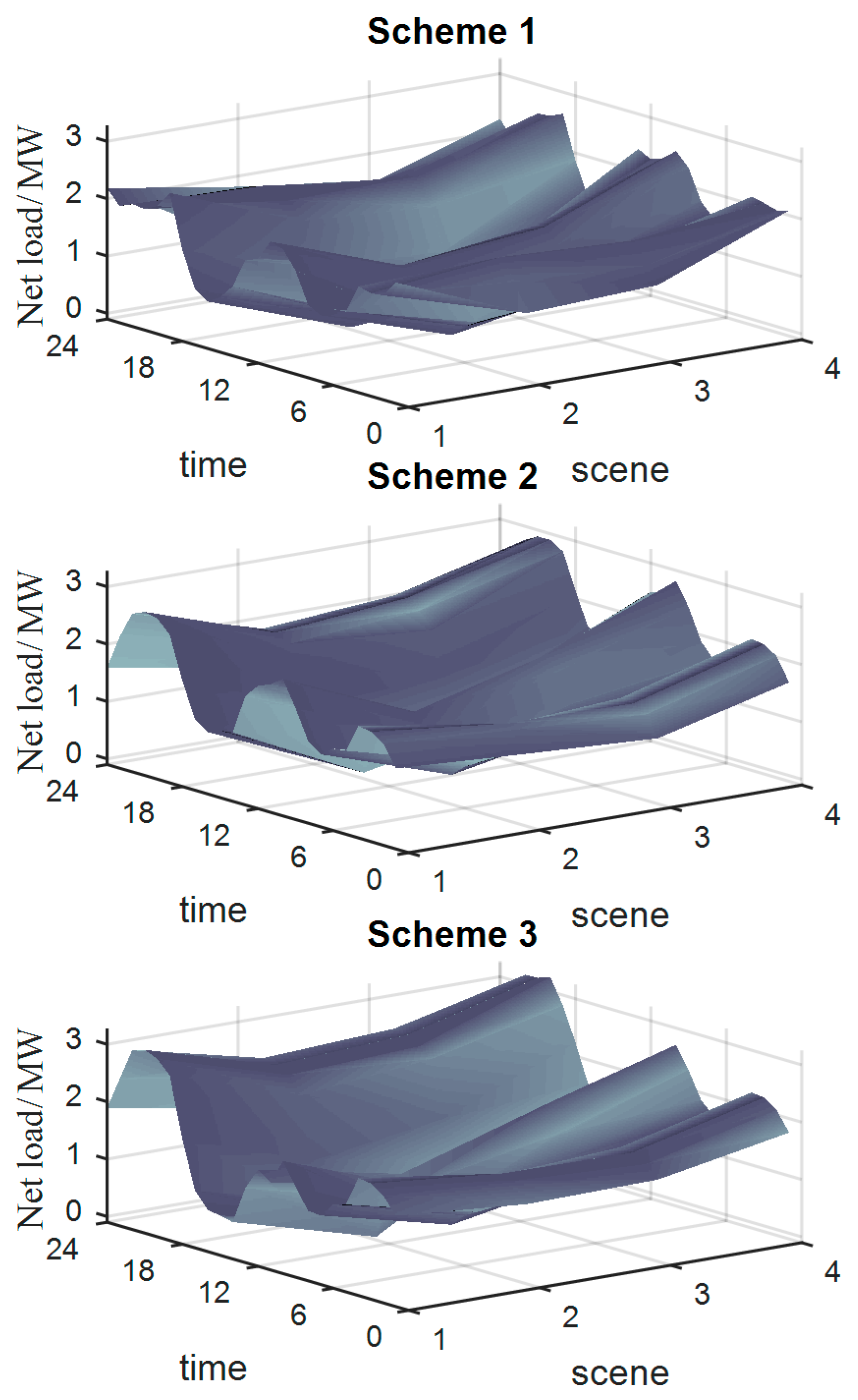
6.2. Analysis of Results

The following three schemes were used for the optimization for DG and the EVCSs.
Scheme 1: Multi-objective planning model of the DG-EVCSs in V2G mode.
Scheme 2: Multi-objective planning model of the DG-EVCSs in the plug-and-charge charging mode.
Scheme 3: Planning model of the DG-EVCSs in V2G mode maximize comprehensive profit.
The results of the optimization of the DG-EVCSs, based on the above three schemes, are shown in Table 3. It lists the optimal planning schemes determined using the time frame of year, including the four scenarios shown in Figure 6. The corresponding DG consumption and charging load acceptance under the three schemes are shown in Table 3.
In the DG planning scheme, 13(10) indicates that 10 distributed generators were installed in node 13, and in the EVCSs planning scheme, 20(309) indicates that the capacity of the charging station at node 20 was 309 kW.
The comprehensive evaluation indices of the three schemes are shown in Table 4.
According to the data in the table, the comprehensive evaluation of Scheme 1 was the best, while that of Scheme 2 was similar to the evaluation of Scheme 3.
The specific indicators of the comprehensive benefits of the three schemes are shown in Table 5, and those of EV charging satisfaction are shown in Table 6.
Compared with Scheme 2, Scheme 1 took into account the V2G effect of the EVs, which helped manage their charging and discharging in an orderly manner, optimize power flow, and improve the consumption capacity of the distribution network to DG. The clean energy consumption of the three schemes is shown in Table 7. Compared with Scheme 2, the planning capacity of Scheme 1 increased by 500 kW, and the consumption of DG increased by 1530 MWh. The increase in DG consumption increased the costs of investment, construction, and maintenance of Scheme 1, but also increased income from government subsidies income and reduces the cost of power from the distribution company owing to the superior power grid.
When the capacities of the EVCSs of the two schemes were compared, the planned capacity of Scheme 1 was found to be higher than that of Scheme 2. Compared with the plug-and-charge charging mode, the V2G mode was more conducive to promoting the acceptance of charging load. Therefore, the EV charging completion of Scheme 1 was 6.023% higher than that of Scheme 2, and its charging load acceptance increased by 392 MWh.
In terms of environmental benefits, Table 7 shows that the scheme considering the V2G mode was conducive to promoting the consumption of DG and the charging load and improving the consumption of clean energy in the distribution network.
In terms of the cost of network loss, compared with Scheme 2, the cost of Scheme 1 was reduced by 3.89%, which indicates that appropriate management of charging and discharging can optimize the power flow and reduce network loss.
In terms of EV charging satisfaction, Scheme 2 used the plug-and-charge charging mode, and thus its unit charging cost was high. Scheme 1 responded to the peak and valley prices by scheduling the charging and discharging loads of the EV; its unit charging cost was thus 8.23% lower than that of Scheme 2. The reduction in unit charging cost and the increase in EV charging completion resulted in a 7.1% increase in EV charging satisfaction in Scheme 1.
Compared with Scheme 1, Scheme 3 considered only the comprehensive benefits, and mainly increased them by expanding the acceptance of EV charging load while ignoring voltage quality and load fluctuation. Because Scheme 3 did not take into account EV charging satisfaction, the demand or it by EV users could not be guaranteed, and the unit charging cost was relatively high. Although the comprehensive benefits increased by 524,370 CNY, the higher charging cost led to a decrease in the willingness of EV users to participate in V2G.
In terms of the system load fluctuation index, the net load fluctuation surfaces of the three schemes are shown in Figure 7.
As shown in Figure 7, the surface of the net load fluctuation of Scheme 1 was the smoothest, and its load fluctuation index was 4.99% lower than that of Scheme 2, which indicates that load fluctuation was suppressed in the V2G mode. In Scheme 3, the excessive acceptance of charging load led to the most serious fluctuation in net load. The load fluctuation index of Scheme 3 reached 662.976 kW, an increase of 31.54% compared with Scheme 1. The voltage quality of Scheme 1 was the highest, whereas the disordered access of charging loads in Scheme 3 not only aggravated the fluctuation of system load, but also causes further deterioration in voltage quality.

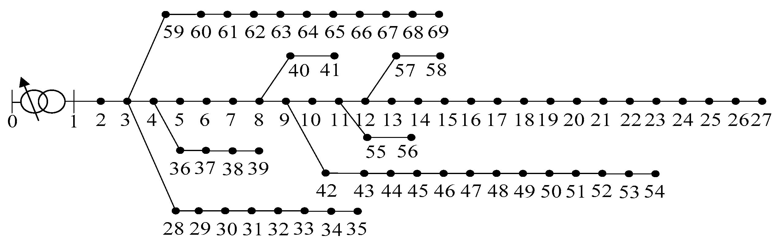
6.3. Case Study Using PG and E-69 Bus Test System

To further verify the effectiveness of the optimization model proposed in this paper, the PG and E-69 bus test system, shown in Figure 8, was used. The system parameters are described in [21].
For the PG and E-69 bus test system, the DWG candidate nodes were nodes 10, 33, and 38, the PV candidate nodes were nodes 21, 50, and 66, and the EVCSs candidate nodes were nodes 14, 32, 40, 45, and 61. The results of optimization of DG and the EVCSs of the three schemes are shown in Table 8, and the corresponding objective functions are shown in Table 9.
According to the data in the table, the comparative advantages and disadvantages of the three schemes were similar to the results of optimization of the IEEE-33 bus test system, and Scheme 1 was the optimal scheme. Based on the results of the PG and E-69 bus test system, the validity of the model proposed in this paper was verified again. The difference between different regions or countries is mainly reflected in the peak or valley electricity prices, which does not affect the overall applicability of the model.

6.4. Comparison of Algorithm Performance

In this paper, the proposed I-HSPSO algorithm and PSO algorithm were tested by using the test functions f1(x)~f4(x), and the optimal value of the four test functions was zero.
f 1 ( x ) = i = 1 n x i 2 ,
f 2 ( x ) = i = 1 n | x i | + i = 1 n | x i | ,
f 3 ( x ) = 0.5 + sin 2 x 1 2 + x 2 2 0.5 [ 1 + 0.001 ( x 1 2 + x 2 2 ) ] 2 ,
f 4 ( x ) = i = 1 n [ x i 2 10 cos ( 2 π x i ) + 10 ] ,
MATLAB was used for programming, the particle swarm size of the algorithm was 50, the number of iterations was 1000, and each algorithm was run independently 100 times. The results of the two algorithms are shown in Table 10.
According to the results for the f1(x) function, the I-HPSO algorithm was superior to the PSO algorithm in terms of searching for single-peak convex functions. The function f2(x) had local extrema around the global optimal value. For such functions with local extremum, compared with the PSO algorithm, the I-HSPSO had stronger global optimization ability. Therefore, all indices in the results of its simulation improved significantly. The function f3(x) had numerous minima and oscillated strongly. The function f4(x) was a nonlinear multi-modal function with jumping peaks, which made it difficult to find the global optimal solution. For such functions as f3(x) and f4(x), which struggled to find the global extremum, the results show that I-HSPSO had a stronger searching ability. Thus, the I-HSPSO algorithm proposed in this paper significantly improved algorithm performance.

7. Conclusions

In this paper, a multi-objective optimization model of the DG-EVCSs was established by considering the V2G technology of EVs. Based on the I-HSPSO algorithm, a bi-level programming model was solved. The conclusions of this study are as follows:
  • Considering the planning of DG and EVCSs in the V2G mode is conducive to improving the consumption of clean energy and optimizing power flow. In this way, network loss and load fluctuations can be reduced, the quality of voltage can be improved, and a scheme with better overall performance can be obtained.
  • In the distribution network with peak and valley prices, the V2G mode can reduce the unit charging cost for EV users, improve EV charging satisfaction, and satisfy the interests of both the distribution company and EV users.
  • The objective here was the comprehensive optimization of four indices such as comprehensive profit, voltage quality, system load fluctuation, and EV charging satisfaction so that the objective function of the planning model was complex, which is conducive to considering multiple demands and improving the comprehensive performance of the planning scheme.
  • The proposed I-HSPSO algorithm converged quickly, and had a strong global optimization ability, because of which it did not easily to fall into the local optimum. Its performance thus improved.

Author Contributions

L.L.: supervision, methodology, original draft; F.X.: formal analysis; Z.H.: methodology; M.W.: review and editing. All authors have read and agreed to the published version of the manuscript.

Funding

This work was supported by Fujian Scholarship to Study Abroad of 2018.

Institutional Review Board Statement

Not applicable.

Informed Consent Statement

Not applicable.

Data Availability Statement

We agree to share our research data, and the data presented in this study are available in this article.

Conflicts of Interest

The authors declare no conflict of interest.

References

  1. Zhao, J.; Xu, Z.; Wang, J.; Wang, C.; Li, J. Robust Distributed Generation Investment Accommodating Electric Vehicle Charging in a Distribution Network. IEEE Trans. Power Syst. 2018, 33, 4654–4666. [Google Scholar] [CrossRef]
  2. Wang, L.; Sharkh, S.; Chipperfield, A. Optimal decentralized coordination of electric vehicles and renewable generators in a distribution network using A∗ search. Int. J. Electr. Power 2018, 98, 474–487. [Google Scholar] [CrossRef]
  3. Erdinc, O.; Tascikaraoglu, A.; Paterakis, N.G.; Dursun, I.; Sinim, M.C.; Catalao, J.P.S. Comprehensive Optimization Model for Sizing and Siting of DG Units, EV Charging Stations, and Energy Storage Systems. IEEE Trans. Smart Grid 2018, 9, 3871–3882. [Google Scholar] [CrossRef]
  4. Yang, H.; Pan, H.; Luo, F.; Qiu, J.; Deng, Y.; Lai, M.; Dong, Z.Y. Operational Planning of Electric Vehicles for Balancing Wind Power and Load Fluctuations in a Microgrid. IEEE Trans. Sustain. Energy 2017, 8, 592–604. [Google Scholar] [CrossRef]
  5. Banol Arias, N.; Tabares, A.; Franco, J.F.; Lavorato, M.; Romero, R. Robust Joint Expansion Planning of Electrical Distribution Systems and EV Charging Stations. IEEE Trans. Sustain. Energy 2018, 9, 884–894. [Google Scholar] [CrossRef] [Green Version]
  6. Zhang, C.; Li, J.; Zhang, Y.J.; Xu, Z. Optimal Location Planning of Renewable Distributed Generation Units in Distribution Networks: An Analytical Approach. IEEE Trans. Power Syst. 2018, 33, 2742–2753. [Google Scholar] [CrossRef]
  7. Luo, L.; Gu, W.; Zhou, S.; Huang, H.; Gao, S.; Han, J.; Wu, Z.; Dou, X. Optimal planning of electric vehicle charging stations comprising multi-types of charging facilities. Appl. Energy 2018, 226, 1087–1099. [Google Scholar] [CrossRef]
  8. Xiang, Y.; Liu, J.; Li, R.; Li, F.; Gu, C.; Tang, S. Economic planning of electric vehicle charging stations considering traffic constraints and load profile templates. Appl. Energy 2016, 178, 647–659. [Google Scholar] [CrossRef] [Green Version]
  9. Sarikprueck, P.; Lee, W.; Kulvanitchaiyanunt, A.; Chen, V.C.P.; Rosenberger, J.M. Bounds for Optimal Control of a Regional Plug-in Electric Vehicle Charging Station System. IEEE Trans. Ind. Appl. 2018, 54, 977–986. [Google Scholar] [CrossRef]
  10. Zhang, H.; Moura, S.J.; Hu, Z.; Qi, W.; Song, Y. Joint PEV Charging Network and Distributed PV Generation Planning Based on Accelerated Generalized Benders Decomposition. IEEE Trans. Transp. Electrif. 2018, 4, 789–803. [Google Scholar] [CrossRef]
  11. Sultana, U.; Khairuddin, A.B.; Sultana, B.; Rasheed, N.; Qazi, S.H.; Malik, N.R. Placement and sizing of multiple distributed generation and battery swapping stations using grasshopper optimizer algorithm. Energy 2018, 165, 408–421. [Google Scholar] [CrossRef]
  12. Buja, G.; Bertoluzzo, M.; Fontana, C. Reactive Power Compensation Capabilities of V2G-Enabled Electric Vehicles. IEEE Trans. Power Electr. 2017, 32, 9447–9459. [Google Scholar] [CrossRef]
  13. Mortaz, E.; Valenzuela, J. Optimizing the size of a V2G parking deck in a microgrid. Int. J. Electr. Power 2018, 97, 28–39. [Google Scholar] [CrossRef]
  14. Zhang, Y.; Hepner, G.F. The Dynamic-Time-Warping-based k-means++ clustering and its application in phenoregion delineation. Int. J. Remote Sens. 2017, 38, 1720–1736. [Google Scholar] [CrossRef]
  15. Vogel, M.A.; Wong, A.K. PFS Clustering Method. IEEE Trans. Pattern Anal. Mach. Intell. 1979, 1, 237–245. [Google Scholar] [CrossRef]
  16. Evangelopoulos, V.A.; Georgilakis, P.S. Optimal distributed generation placement under uncertainties based on point estimate method embedded genetic algorithm. IET Gener. Transm. Distrib. 2014, 8, 389–400. [Google Scholar] [CrossRef] [Green Version]
  17. Luo, Z.; Hu, Z.; Song, Y.; Yang, X.; Wu, J. Study on Plug-in Electric Vehicles Charging Load Calculating. Autom. Electr. Power Syst. 2011, 14, 36–42. [Google Scholar]
  18. Han, X.; Zhao, S.; Wei, Z.; Bai, W. Planning and Overall Economic Evaluation of Photovoltaic-Energy Storage Station Based on Game Theory and Analytic Hierarchy Process. IEEE Access 2019, 7, 110972–110981. [Google Scholar] [CrossRef]
  19. Collotta, M.; Pau, G.; Maniscalco, V. A Fuzzy Logic Approach by Using Particle Swarm Optimization for Effective Energy Management in IWSNs. IEEE Trans. Ind. Electron. 2017, 64, 9496–9506. [Google Scholar] [CrossRef]
  20. Baran, M.E.; Wu, F.F. Network reconfiguration in distribution systems for loss reduction and load balancing. IEEE Trans. Power Deliv. 1989, 4, 1401–1407. [Google Scholar] [CrossRef]
  21. Baran, M.E.; Wu, F.F. Optimal capacitor placement on radial distribution systems. IEEE Trans. Power Deliv. 2002, 4, 725–734. [Google Scholar] [CrossRef]
Figure 1. Curves of wind speed, light intensity, and demand for load.
Processes 09 00018 g001
Figure 2. The charging and discharging time distribution of EV.
Processes 09 00018 g002
Figure 3. Algorithm flow of I-HSPSO.
Processes 09 00018 g003
Figure 4. Flowchart of bi-level programming model.
Processes 09 00018 g004
Figure 5. IEEE 33-bus distribution network.
Processes 09 00018 g005
Figure 6. Wind speed, light intensity and load scenarios.
Processes 09 00018 g006
Figure 7. Multi-scenario net load fluctuation surfaces.
Processes 09 00018 g007
Figure 8. PG and E 69 bus test system.
Processes 09 00018 g008
Table 1. Peak and valley price.
Electricity Cost Price/(CNY/kWh)Electricity Sale Price/(CNY/kWh)Charging Cost of EV/(CNY/kWh)Discharge Compensation Coefficient/(CNY/kWh)
Peak time0.61291.111.52.20
Normal time0.44300.681.01.23
Valley time0.21890.350.750.35
Table 2. Cost parameters of environmental pollution.
Contaminantxs/(kg/MWh)as/(CNY/kg)bs/(CNY/kg)
CO2639.20.010.02
SO23.5871.006.00
NOx1.5442.008.00
Table 3. Optimal results of allocation of different schemes.
SchemeOptimal Allocation ResultsCapacity/kW
Scheme 1DG13(10).23(8).31(10).7(7)3500
EVCSs20(309).4(254).8(288).14(211).29(296)1358
Scheme 2DG13(10).23(6).31(7).28(7)3000
EVCSs20(290).4(150).8(387).14(248).29(173)1248
Scheme 3DG13(8).23(3).31(9).7(1).21(9).28(7)3700
EVCSs20(327).4(293).8(348).14(202).29(291)1461
Table 4. Comprehensive evaluation indices of the three schemes.
SchemeScheme 1Scheme 2Scheme 3
Comprehensive profit/10,000 CNY1199.2381204.6781251.675
Voltage quality/pu0.8450.8310.823
System load fluctuation/kW504.026530.489662.976
Charging satisfaction of EV/%0.9110.8400.866
Comprehensive evaluation indices/pu0.9330.8970.899
Table 5. Specific indicators of comprehensive benefits.
SchemeScheme 1Scheme 2Scheme 3
Electricity sale benefits/10,000 CNY1514.4171514.4171514.417
Charging station sales revenue/10,000 CNY550.484603.089668.442
Electricity purchasing cost/10,000 CNY587.752648.469658.807
Investment and construction cost/10,000 CNY422.985388.860433.661
Maintenance cost/10,000 CNY47.44241.75641.501
Government subsidy benefits/10,000 CNY144.806130.280167.040
System network loss cost/10,000 CNY38.97940.55642.882
Environmental benefits/10,000 CNY86.68976.53378.627
Table 6. Specific indicators of EV charging satisfaction.
SchemeScheme 1Scheme 2Scheme 3
Charging completion of EV/%86.16280.13988.299
Unit charging cost of EV/(CNY/kWh)1.0601.1551.171
Table 7. Clean energy consumption.
SchemeScheme 1Scheme 2Scheme 3
Consumption of DG/MWh12,06710,53710,656
Total acceptance of charging load/MWh561252205751
Table 8. Optimization results.
SchemeOptimal Allocation ResultsCapacity/kW
Scheme 1DG10(9).33(2).38(10).21(1).50(5).66(4)3100
EVCSs14(259).31(237).40(257).45(258).61(299)1310
Scheme 2DG10(6).33(2).38(10).21(3).50(10)3100
EVCSs14(232).31(187).40(245).45(150).61(242)1056
Scheme 3DG33(7).38(10).21(8).50(10).66(10)4500
EVCSs14(442).31(439).40(331).45(308).61(389)1909
Table 9. Comprehensive evaluation index.
SchemeScheme 1Scheme 2Scheme 3
Comprehensive profit/10,000 CNY1147.3661202.4221320.579
Voltage quality/pu0.9900.9890.987
System load fluctuation/kW492.478524.166866.618
Charging satisfaction of EV/%0.9040.8290.870
Comprehensive evaluation indices/pu0.9050.8800.886
Table 10. Results of algorithm simulation.
FunctionAlgorithmBest ValueWorst ValueMean Value
f1PSO3.832 × 10−232.194 × 10−52.577 × 10−7
I−HSPSO9.001 × 10−249.168 × 10−84.258 × 10−9
f2PSO0.1795143.27414.165
I−HSPSO3.745 × 10−41.992 × 10−11.849 × 10−2
f3PSO9.368 × 10−130.0090.004
I−HSPSO00.0096.802 × 10−4
f4PSO3.98029.84912.696
I−HSPSO3.836 × 10−249.9493.872
Publisher’s Note: MDPI stays neutral with regard to jurisdictional claims in published maps and institutional affiliations.

