PID Tuning Method Based on IMC for Inverse-Response Second-Order Plus Dead Time Processes

Abstract

This work addresses a set of tuning rules for PID controllers based on Internal Model Control (IMC) for inverse-response second-order systems with dead time. The transfer function, and some time-response characteristics for such systems are first described. Then, the IMC-based methodology is developed by using an optimization objective function that mixes performance and robustness. A correlation that minimizes the objective function and that allows the user to compute the controller’s tuning parameter is found. The obtained expressions are mathematically simple, which facilitate their application in a ten-step systematic methodology. Finally, the proposed tuning method is compared to other well-known tuning rules that have been reported in literature, for a wide range of parameters of the process. The performance achieved with the proposed method is very good not only for disturbance rejection but for set-point tracking, when considering a wide-range of parameters of the process’ transfer function.

1. Introduction

Inverse response or non-minimum-phase systems have at least one zero located at the right-hand side of the complex plane [1]. Their time response to a step input goes, at the beginning, towards the opposite direction of the steady-state value [2]. Such behavior appears due to the combination of two opposite-dynamics phenomena: A small-gain fast-dynamics responsible for the inverse response, and a slow-dynamics with higher gain, which dominates the transient response [3,4,5].

Since the inverse response phenomenon presents some similar characteristics to those in dead-time systems, it is usual to find tuning techniques with Smith predictor-like structures [6,7]. Other tuning techniques present the model of the non-minimum-phase zero as dead time, which allows one to use traditional tuning techniques developed for time-delayed systems [8]; conservative controllers are obtained with such an approximation [9,10,11]. Another traditional way to deal with inverse response dynamics is to reduce the order of the system and get a first-order model, which allows one to obtain PI controllers; however, these controllers can cause slower transient responses than the aforementioned techniques [12].

The development of Proportional-Integral (PI) and Proportional-Integral-Derivative (PID) controllers for inverse response processes started around the 1970s. Waller and Nygardas [13] compared lead-lag compensators to the conventional PID tuning proposed by Ziegler and Nichols [14]. Then, Scali and Rachid [15], Luyben [16], Chien et al. [17], and Sree and Chidambaram [18], among others, reported different tuning techniques for PI/PID controllers used for inverse-response systems by considering, in general, set-point changes. One can find some references, such as Chen and Seborg [19], Shamsuzzoha and Lee [20], and Pai et al. [9] that developed tuning equations for disturbance rejection. More recently, several PID tuning or controller design methods for processes whose dynamics include inverse-response, time-delay, and integrating characteristics have been developed [21,22,23,24,25,26]. Other authors gone beyond the PID controller and proposed the use of fractional control for non-minimum phase plus dead time systems [27], and Sliding Mode Controllers applied to high-order long dead-time inverse-response processes [28].

Other PID design methods based on frequency response techniques have been developed. For instance, Luyben [29] presented a PI controller tuning procedure for an inverse-response integrating process; the author states that the controller tuning process for this kind of complex dynamics is not a trivial task. Chen and Seborg [19] developed a design method for PID controllers based on direct synthesis; they demonstrated that the design method works very good for several processes, including those with non-minimum phase characteristics that appear when Pade’s approximation is used for systems with dead time. Such approximation induces an additional modeling error, which implies a decrease in the system’s bandwidth [30]. Alfaro et al. [31] used a nondimensional version of equations proposed by Chen and Seborg [19] and found expressions in order to compute the minimum value of the tuning parameter, ${\tau }_c$, which bounds the maximum sensitivity.

Internal Model Control (IMC) has been used as an alternative for designing and tuning PID controllers since 1980s [30]. It has resulted to be of particular interest in industry together with the PID algorithm [32], since the equations for the controller’s parameters can be obtained from the transfer function of the process and the desired behavior of the closed-loop response; in most cases, only the closed-loop time constant is required as the user-defined tuning parameter, considering an appropriate trade-off between performance and robustness [20,33,34,35,36,37]. Additional works, regarding IMC, that have been developed more recently can be found in [38,39,40,41,42,43,44].

This work addresses the design of a tuning methodology for PID controllers, for inverse-response second-order plus dead time processes, extending the work of Chien and Fruehauf [45], which has been recently studied in [46], by using dimensional analysis and experimental design. The development of the tuning technique considers the optimization of an objective function that combines performance and robustness indexes: the Integral of the Absolute Value of the Error (IAE) and the Integral of the change in the Manipulated Variable (IMV). The obtained expressions are simple and can be applied by using the proposed ten-step methodology. The performance of a controller tuned with this method excels the performance offered by other well-known techniques for a wide range of parameters of the process.

The first section contains a description of process’ time response. Then, the design process of the tuning rules is addressed, by using dimensional analysis and experimental design. The third section contains the application methodology and the performance comparison for a controller tuned with the new rules and other tuning methods. Then, the robustness analysis for the variability of parameters is performed. Finally, the conclusions are presented.

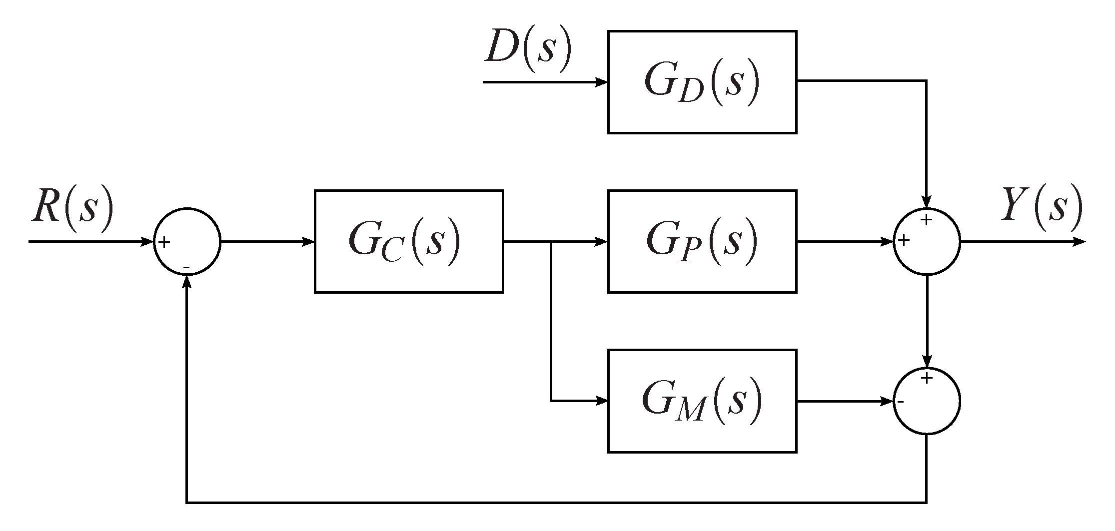
2. Inverse Response Second Order Plus Dead Time System Model

The transfer function of an inverse-response second-order system, with total time delay $\theta$, can be written as

$$G\left(s\right)=[G_1\left(s\right)+G_2\left(s\right)]e^{-\theta s};$$

(1)

where

$$G_1\left(s\right)={\displaystyle \frac{K_1}{{\tau }_{1}s+1}},$$

(2)

$$G_2\left(s\right)={\displaystyle \frac{-K_2}{{\tau }_{2}s+1}},$$

(3)

are the transfer functions of two opposite-dynamics phenomena: A small-gain fast-dynamics part (3), and a slow-dynamics part with higher gain (2). $K_1$ and $K_2$ are the gains, and ${\tau }_1$ and ${\tau }_2$ are the time constants. Substituting (2) and (3) into (1) yields

$$G\left(s\right)=\frac{(K_1{\tau }_2-K_2{\tau }_1)s+(K_1-K_2)}{({\tau }_{1}s+1)({\tau }_{2}s+1)}{e}^{-\theta s}.$$

(4)

As it can be seen in (4), the process’ transfer function only considers the case with real different poles because the dynamics comes from parallel balances [47]; this is a common case in industrial processes containing boilers, heat exchangers, tanks, distillation columns, chemical reactors, waste incinerators, among others [2,47].

Operating expressions in (4) yields the transfer function of the process which is given by

$$G\left(s\right)=K\frac{(1-\eta s)}{({\tau }_{1}s+1)({\tau }_{2}s+1)}{e}^{-\theta s},$$

(5)

where $K=K_1-K_2$, and $\eta ={\displaystyle \frac{(K_2{\tau }_1-K_1{\tau }_2)}{(K_1-K_2)}}$, $\eta >0$.

For this process, at the beginning, the time response slope’s sign is opposite to the sign of the gain, and as $\eta$ increases, so does the inverse-response behaviour; then, control issues arise due to the fact that the non-minimum phase zero is closer to the imaginary axis [4,15,48,49]. Adding a left-hand side pole into (5) decreases this inverse-response effect, but the settling time increases. When there are multiple non-minimum phase zeros, multiple inversions appear; however, such a system is not commonly found.

3. Design of Tuning Rules

3.1. Internal Model Control

Internal Model Control (IMC) is a technique that uses a simulation of the process, running in parallel [30], as depicted in Figure 1; where: $R\left(s\right)$ is the input reference, $D\left(s\right)$ is the disturbance signal, $Y\left(s\right)$ is the output of the system, $G_P\left(s\right)$ is the process transfer function, $G_D\left(s\right)$ is the transfer function that relates the output and the disturbance, $G_C\left(s\right)$ is the controller transfer function, and $G_M\left(s\right)$ is the model of the process that is simulated in parallel. The IMC methodology requires the transfer function of the model of the process be written as:

$$G_M\left(s\right)=G_{M^{+}}\left(s\right)G_{M^{-}}\left(s\right),$$

(6)

where $G_{M^{+}}\left(s\right)$ is a transfer function containing all the non-minimum phase zeros and dead time, and $G_{M^{-}}\left(s\right)$ contains the minimum-phase elements of the system. Then, the IMC controller can be defined in terms of the invertible part of the transfer function and a user-specified low-pass filter $f\left(s\right)$, as follows

$$G_{IMC}=G_{M^{-}}^{-1}\left(s\right)f\left(s\right).$$

(7)

The IMC controller’s structure can be reduced to a classical PI/PID control structure. For this purpose, Chien and Fruehauf [45] defined the filter’s function, for first and second-order systems (without integrator), as follows

$$f\left(s\right)={\displaystyle \frac{1}{{\tau }_{c}s+1}}.$$

(8)

They used a parallel PID controller structure which is given by

$$G_C\left(s\right)=K_c\left(1+{\displaystyle \frac{1}{T_{i}s}}+T_{d}s\right).$$

(9)

These authors obtained equations for the tuning parameters, which are given for an inverse response second order plus dead time system by [45]

$$\begin{array}{cc}\hfill K_c& ={\displaystyle \frac{{\tau }_1+{\tau }_2+{\displaystyle \frac{\eta \theta }{{\tau }_c+\eta +\theta }}}{K({\tau }_c+\eta +\theta )}},\hfill \end{array}$$

(10)

$$\begin{array}{cc}\hfill T_i& ={\tau }_1+{\tau }_2+{\displaystyle \frac{\eta \theta }{{\tau }_c+\eta +\theta }},\hfill \end{array}$$

(11)

$$\begin{array}{cc}\hfill T_d& ={\displaystyle \frac{\eta \theta }{{\tau }_c+\eta +\theta }}+{\displaystyle \frac{{\tau }_1{\tau }_2}{{\tau }_1+{\tau }_2+{\displaystyle \frac{\eta \theta }{{\tau }_c+\eta +\theta }}}},\hfill \end{array}$$

(12)

where ${\tau }_c$ is the tuning parameter.

3.2. Optimization Objective Function

In this work, we use the optimization of a performance index that combines the Integral of the Absolute Value of the Error (IAE) and the Integral of the change in the Manipulated Variable (IMV). The controller’s main operation in this case favors disturbance rejection (load regulation); however, reference tracking performance is also evaluated. The objective function is then given by

$$OF={\int }_0^{\infty }\left|e\left(t\right)\right|dt+\gamma {\int }_0^{\infty }\left|{\displaystyle \frac{dMV\left(t\right)}{dt}}\right|dt.$$

(13)

The first term in (13) is the IAE, and the second term is the IMV multiplied by a suppression factor $\gamma$. Increasing or decreasing $\gamma$ allows one to modify the weight on the manipulated variable; for instance, when $\gamma =1$, both, the IAE and IMV are of the same importance, and when $\gamma =0$ only the IAE is considered. Several authors have used this type of objective function in order to measure the performance of different control strategies [50,51]; typical values of the suppression factor are $0\le \gamma \le 8$ [52,53].

3.3. Scaling and Nondimensionalization

In order to reduce the amount of parameters to be optimized, Equations (5), (10)–(12) are scaled using dimensional analysis techniques, allowing us to go from the 4 parameters contained in (5) to the 3 parameters found in Equations (18)–(20); this reduces the number of simulation runs and computation time. Nondimensional equations are written in the form proposed in [49,54] and given by

$$\begin{array}{cc}\hfill \widehat{G}\left(\widehat{s}\right)& ={\displaystyle \frac{(-\widehat{\eta }\widehat{s}+1)e^{-\widehat{\theta }\widehat{s}}}{(\widehat{s}+1)({\widehat{\tau }}_2\widehat{s}+1)}},\hfill \end{array}$$

(14)

$$\begin{array}{cc}\hfill K_{c}K& ={\displaystyle \frac{(1+{\widehat{\tau }}_2)({\widehat{\tau }}_c+\widehat{\eta }+\widehat{\theta })+\widehat{\eta }\widehat{\theta }}{{({\widehat{\tau }}_c+\widehat{\eta }+\widehat{\theta })}^2}},\hfill \end{array}$$

(15)

$$\begin{array}{cc}\hfill {\widehat{T}}_i& ={\displaystyle \frac{(1+{\widehat{\tau }}_2)({\widehat{\tau }}_c+\widehat{\eta }+\widehat{\theta })+\widehat{\eta }\widehat{\theta }}{({\widehat{\tau }}_c+\widehat{\eta }+\widehat{\theta })}},\hfill \end{array}$$

(16)

$$\begin{array}{cc}\hfill {\widehat{T}}_d& ={\displaystyle \frac{\widehat{\eta }\widehat{\theta }}{({\widehat{\tau }}_c+\widehat{\eta }+\widehat{\theta })}}+{\displaystyle \frac{{\widehat{\tau }}_2({\widehat{\tau }}_c+\widehat{\eta }+\widehat{\theta })}{(1+{\widehat{\tau }}_2)({\widehat{\tau }}_c+\widehat{\eta }+\widehat{\theta })}},\hfill \end{array}$$

(17)

where:

$$\begin{array}{cc}\hfill \widehat{\eta }& =\frac{\eta }{{\tau }_1},\hfill \end{array}$$

(18)

$$\begin{array}{cc}\hfill {\widehat{\tau }}_2& =\frac{{\tau }_2}{{\tau }_1},\hfill \end{array}$$

(19)

$$\begin{array}{cc}\hfill \widehat{\theta }& =\frac{\theta }{{\tau }_1},\hfill \end{array}$$

(20)

$$\begin{array}{cc}\hfill \widehat{s}& ={\tau }_{1}s.\hfill \end{array}$$

(21)

This can be interpreted as scaling in time or frequency domains. The typical values for the ratios between the parameters can be found in literature and are given by [9,49]

$$\begin{array}{c}\hfill 0.1\le {\displaystyle \frac{{\tau }_2}{{\tau }_1}}\le 0.9,\end{array}$$

(22)

$$\begin{array}{c}\hfill 0.1\le {\displaystyle \frac{\eta }{{\tau }_1}}\le 4,\end{array}$$

(23)

$$\begin{array}{c}\hfill 0.01\le {\displaystyle \frac{\theta }{{\tau }_1}}\le 1.\end{array}$$

(24)

A central composite experimental design (uniform and circumscribed for rotatability) was designed in order to provide appropriated values of $\frac{{\tau }_2}{{\tau }_1}$, $\frac{\eta }{{\tau }_1}$, and $\frac{\theta }{{\tau }_1}$ for each simulation run. This type of experimental design is selected since it can take account of curvature in a response [55], i.e., a quadratic surface can be adjusted to the data provided. Gutierrez and de la Vara [56] stated that in order to get accurate predictions, values of $R^2\ge 70$ % are expected; since the selection of parameters out of ranges provided in expressions (22)–(24) cannot guarantee such $R^2$ value, we developed the tuning method for the given ranges, which were selected as in [9,49].

Castellanos and Castrillón [57] presented an expression that allows one to compute the limit value that can be assigned to the controller’s parameter in order to get a fast response, without compromising stability. Additionally, they reported a typical polynomial-like correlation that allows one to obtain the value of the tuning parameter that minimizes only the IAE. Such expressions are given by [57]

$$\begin{array}{cc}\hfill {\widehat{\tau }}_{cult}=& -0.148557+0.903364{\widehat{\tau }}_2+0.331659\widehat{\eta }+0.390943{\widehat{\tau }}_2\widehat{\eta }-0.19992{\widehat{\tau }}_2\widehat{\theta }\hfill \\ \hfill & +0.384281\widehat{\eta }\widehat{\theta }-0.305025{\widehat{\tau }}_2^2-0.0157256{\widehat{\eta }}^2-0.207827{\widehat{\theta }}^2,\hfill \end{array}$$

(25)

$$\begin{array}{cc}\hfill {\widehat{\tau }}_{cIAE}=& -0.540626+2.11424{\widehat{\tau }}_2+0.735044\widehat{\eta }+1.6421\widehat{\theta }+0.640022{\widehat{\tau }}_2\widehat{\eta }\hfill \\ \hfill & +0.341155\widehat{\eta }\widehat{\theta }-1.66075{\widehat{\tau }}_2^2-0.0294597{\widehat{\eta }}^2-0.962638{\widehat{\theta }}^2,\hfill \end{array}$$

(26)

where ${\widehat{\tau }}_{cult}$ is the minimum allowable value of the tuning parameter; i.e., lower values of ${\widehat{\tau }}_{cult}$ make the system exhibit unstable behavior; and ${\widehat{\tau }}_{cIAE}$ is the value of the tuning parameter that minimizes the IAE. In the present work we develop the equations for $\gamma >0$ which allow one to use the combined index.

3.4. Tuning Parameter Computation

It is desired to obtain a new expression in order to relate the controller’s tuning parameter that minimizes the objective function and the ultimate value that can be chosen in order to obtain a stable response:

$${\widehat{\tau }}_{cOF}=f({\widehat{\tau }}_{cult},\gamma ).$$

(27)

A simulation environment was developed using MATLAB^®/Simulink^®. This computational tool allows one to find the value of the objective function for each data set of parameters of the process’ transfer function and $\gamma$. Since we used a central composite experimental design for rotatability, the optimization tool correspond to the steepest-descent gradient method [58].

The starting value of ${\widehat{\tau }}_c$ for each simulation was obtained from (25); the minimum assigned value for this parameter matched the limit value to obtain a stable system. The simulations considered unit-step changes in the disturbance variable (disturbance rejection). At the end of the simulation process, we obtained data shown in

Table A1. Experimental design results.

${\widehat{\mathit{\tau }}}_2$	$\widehat{\mathit{\eta }}$	$\widehat{\mathit{\theta }}$	${\widehat{\mathit{\tau }}}_{\mathit{cult}}$	${\widehat{\mathit{\tau }}}_{\mathit{cFO}|0}$	${\widehat{\mathit{\tau }}}_{\mathit{cFO}|1}$	${\widehat{\mathit{\tau }}}_{\mathit{cFO}|2}$	${\widehat{\mathit{\tau }}}_{\mathit{cFO}|3}$	${\widehat{\mathit{\tau }}}_{\mathit{cFO}|4}$	${\widehat{\mathit{\tau }}}_{\mathit{cFO}|5}$	${\widehat{\mathit{\tau }}}_{\mathit{cFO}|6}$	${\widehat{\mathit{\tau }}}_{\mathit{cFO}|7}$	${\widehat{\mathit{\tau }}}_{\mathit{cFO}|8}$
0.26	0.89	0.21	0.49	1.10	1.70	1.94	2.10	2.10	2.10	2.57	2.57	3.44
0.26	0.89	0.80	0.55	1.66	2.09	2.39	2.63	2.63	2.75	2.88	2.88	2.88
0.26	3.21	0.21	1.50	2.96	4.25	4.69	5.33	5.87	6.59	7.22	8.05	8.05
0.26	3.21	0.80	2.11	4.07	4.64	5.35	5.70	5.92	6.04	6.90	6.90	7.41
0.74	0.89	0.21	0.89	1.56	2.28	2.65	3.22	3.22	3.41	3.41	3.55	3.55
0.74	0.89	0.80	0.93	2.17	2.54	3.01	3.38	3.55	3.87	4.19	4.19	4.19
0.74	3.21	0.21	2.38	4.22	5.32	5.94	6.46	6.88	6.88	7.81	7.81	7.81
0.74	3.21	0.80	2.87	5.20	5.57	6.40	7.02	7.34	7.75	8.13	8.39	8.70
0.10	2.05	0.50	0.97	2.09	2.74	2.99	3.54	3.78	4.40	4.89	5.36	5.82
0.90	2.05	0.50	2.04	3.51	4.09	4.75	5.27	5.75	5.99	6.13	6.13	6.35
0.50	0.10	0.50	0.19	0.71	1.23	1.62	1.85	1.96	2.00	2.00	2.00	2.10
0.50	4.00	0.50	2.80	5.21	5.94	7.08	7.32	7.60	7.96	8.24	9.60	8.68
0.50	2.05	0.01	1.28	2.16	3.10	5.39	5.80	5.80	5.86	5.86	5.80	5.86
0.50	2.05	0.01	1.71	3.50	3.10	4.48	4.88	5.25	5.59	5.59	5.59	5.59
0.50	2.05	0.50	1.54	3.08	3.71	4.23	4.63	4.97	4.97	4.97	5.35	5.35

(Appendix A) that contains the value of ${\widehat{\tau }}_c$ that minimizes $OF$ for each data set of the process’ transfer function (from the experimental design) and values of $0\le \gamma \le 8$. We found that no significant changes in ${\widehat{\tau }}_{cOF}$ were obtained for $\gamma >4$; therefore, the range $0\le \gamma \le 4$ was selected and Figure 2 shows ${\widehat{\tau }}_{cOF}$ for different values of ${\widehat{\tau }}_{cult}$ considering such range for $\gamma$.

Using the information provided in Figure 2, data were fitted using a linear regression, and the polynomial represents a straight line passing through the origin. The correlations obtained are given by

$$\begin{array}{c}\hfill {\widehat{\tau }}_{cFO|0}=1.9044{\widehat{\tau }}_{cult},\end{array}$$

(28)

$$\begin{array}{c}\hfill {\widehat{\tau }}_{cFO|1}=2.2745{\widehat{\tau }}_{cult},\end{array}$$

(29)

$$\begin{array}{c}\hfill {\widehat{\tau }}_{cFO|2}=2.6513{\widehat{\tau }}_{cult},\end{array}$$

(30)

$$\begin{array}{c}\hfill {\widehat{\tau }}_{cFO|3}=2.8867{\widehat{\tau }}_{cult},\end{array}$$

(31)

$$\begin{array}{c}\hfill {\widehat{\tau }}_{cFO|4}=3.0550{\widehat{\tau }}_{cult}.\end{array}$$

(32)

Equations (28)–(32) are of the form

$${\widehat{\tau }}_{cOF}=m_{OF}{\widehat{\tau }}_{cult},$$

(33)

where $m_{OF}$ is the slope of the line that relates ${\widehat{\tau }}_{cOF}$ and ${\widehat{\tau }}_{cult}$; $m_{OF}$ addtionally represents a stability margin for the system.

When $\gamma$ increases, the value of the slope increases, and ${\widehat{\tau }}_{cOF}$ increases, which make the system more robust. This characteristic allows getting a safety factor for the closed-loop system with respect to an ultimate value ${\widehat{\tau }}_{cult}$; if this value is reached, the time response would acquire sustained oscillations (marginal stability).

In order to measure the goodness of fit, some statistics need to be computed: the correlation coefficient (R), that measures the linear correlation between two variables; the coefficient of determination ($R^2$), that indicates the proportion of the variance that can be explained from the obtained model; and Durbin-Watson, that is used to check if there is a linear autocorrelation among the residuals of the model.

Table 1. Statistics for the objective function $O{F}_{\gamma |i}$ (linear regressions in Figure 2).

${\mathit{OF}}_{\mathit{\gamma }|\mathit{i}}$	R (Fraction)	${\mathit{R}}^2$ (%)	Durbin-Watson (Nondimensional)
$O{F}_{\gamma |0}$	0.9965	99.31	2.16
$O{F}_{\gamma |1}$	0.9918	98.36	2.02
$O{F}_{\gamma |2}$	0.9872	97.46	2.19
$O{F}_{\gamma |3}$	0.9857	97.15	2.42
$O{F}_{\gamma |4}$	0.9865	97.33	2.47

shows the statistics results; it can be noticed that values greater than 0.98 were obtained for R, and values greater than 97 % were obtained for $R^2$; this shows a strong goodness of fit. Values between 2 and 2.5 were obtained for Durbin-Watson, which shows that there is no linear autocorrelation among the model’s residuals.

It is necessary to obtain an expression that relates the value of $m_{OF}$ with $\gamma$. This is done using the value $m_{OFi}$ found in the linear Equations (28)–(32) for different values of $\gamma$. So, for $0\le \gamma \le 4$ we get the plot shown in Figure 3.

Using a nonlinear regression for the plot in Figure 3 we get the expression $m_{OF}=f\left(\gamma \right)$, as follows

$$m_{OF}={\displaystyle \frac{3.3650}{1+e^{\left(-{\displaystyle \frac{\gamma -0.4956}{1.9491}}\right)}}}.$$

(34)

The best fit was given by a sigmoid function; the goodness-of-fit is measured again by using R and $R^2$, both with values greater than 0.99 and 99%, respectively, as shown in

Table 2. Statistics for $m_{OF}\left(\gamma \right)$ (nonlinear regression of Figure 3).

	R (Fraction)	${\mathit{R}}^2$ (%)
$m_{OF}\left(\gamma \right)$	0.9994	99.89

.

Equation (34) shows the relation between the stability margin $m_{OF}$ and the suppression factor $\gamma$. Then, an expression that allows computing the nondimensional optimal value of the controller’s tuning parameter in a direct way is given by

$${\widehat{\tau }}_{cOF}=m_{OF}{\widehat{\tau }}_{cult}.$$

(35)

Finally, Equations (10)–(12) are used to compute the PID controller’s parameters using ${{\tau }_c}_{OF}$, with units of time, that is computed as

$${{\tau }_c}_{OF}={\widehat{\tau }}_{cOF}{\tau }_1.$$

(36)

4. Application Methodology

The application of the Castellanos-Castrillón-Vásquez (CCV) PID tuning method for inverse-response second-order plus dead time systems can be summarized in the following ten steps; Figure 4 shows the methodology in the algorithm form.

• Determine the transfer function of the inverse response second order plus dead time system and write it in the form of (5).
• Verify that the transfer function’s parameters are within the specified ranges, established in (22)–(24); this method is valid only for such ranges.
• Compute the nondimensional parameters of the process by using Equations (18)–(20).
• Compute ${\widehat{\tau }}_{cult}$ by using (25).
• Select the value of $\gamma$, depending on the user’s needs. If $\gamma =0$, $OF=IAE$.
• To compute $m_{OF}$ by using (34), if $\gamma \ne 0$.
• Compute ${\widehat{\tau }}_{cOF}$ by using (35).
• Compute ${{\tau }_c}_{OF}$ by using (36).
• Compute the controller’s parameters with ${{\tau }_c}_{OF}$ using (10)–(12).
• Check if the controller meets the desired performance.

If the desired performance is not met, the user can go back to Step 5 and change the value of $\gamma$ adjusting the index in (13), which accounts for performance of the controlled variable and behaviour of the manipulated variable; high values $\gamma$ are useful to protect the actuators, providing more conservative responses.

5. Discussion on Performance Analysis

This section contains a comparison for the performance of a controller tuned with the new proposed CCV method and three other well-known techniques. There are several PI/PID controller tuning techniques [59], which are used for processes with specific dynamics characteristics. Regarding, inverse response processes, one can find that even recent literature still uses classical methods for comparison purposes or reference them as still valid and used for adjusting controller parameters. One can find recent literature in which new tuning methods, developed by Waller and Nygardas (WN) [13] and Chien, Chung, Chen, and Chuang (CCCC) [17] for inverse response systems, are compared to traditional methods; see for instance [60,61]. Additionally, one can find several works that compare the performance with one of the most traditional tuning methods developed by Ziegler and Nichols (ZN) [14] during the 1940s, see for instance [62,63,64]. The performance indexes are given by

• ${\displaystyle IAE={\int }_0^{\infty }\left|e\left(t\right)\right|dt}$, $[=]$ %TO·UT;
• ${\displaystyle ISE={\int }_0^{\infty }{e}^2\left(t\right)dt}$, $[=]$(%TO)${}^2$·UT;
• ${\displaystyle IMV={\int }_0^{\infty }\left|{\displaystyle \frac{dMV\left(t\right)}{dt}}\right|dt}$, $[=]$ %CO;
• $MP$ (maximum peak), $[=]$ %TO;

where %TO: percentage of transmitter output, %CO: percentage of controller output, UT: units of time.

A central composite experimental design, as explained in the scaling section, was implemented in order to select a set of parameters of the process’ transfer function to test the performance and robustness of the closed-loop, for each controller, over a wide range of values. These values are within the defined ranges of the ratios given by (22)–(24). A tag $P_i$ was assigned to each set, and their values are shown in

Table 3. Simulation parameters sets for performance and robustness analysis.

Parameters	${\widehat{\mathit{\tau }}}_2$	$\widehat{\mathit{\eta }}$	$\widehat{\mathit{\theta }}$
$P_1$	0.2622	3.2095	0.2107
$P_2$	0.5000	2.0500	0.0100
$P_3$	0.5000	2.0500	1.0000
$P_4$	0.5000	4.0000	0.5050
$P_5$	0.7378	3.2095	0.7993

; these parameters are a subset extracted from the experimental region.

For each simulation, the system was excited with a unit-step input for changes in the disturbance and changes in the set-point. A value of $\gamma =4$ was assigned for all the simulations in order to penalize the behavior of the manipulated variable, considered in the second term of the optimization objective function (13).

Table 4. Controller parameters for sets $P_1$, $P_2$, $P_3$, $P_4$, $P_5$.

Set	CCV			WN			ZN			CCCC
	${\mathit{K}}_{\mathit{c}}\mathit{k}$	${\widehat{\mathit{T}}}_{\mathit{i}}$	${\widehat{\mathit{T}}}_{\mathit{d}}$	${\mathit{K}}_{\mathit{c}}\mathit{k}$	${\widehat{\mathit{T}}}_{\mathit{i}}$	${\widehat{\mathit{T}}}_{\mathit{d}}$	${\mathit{K}}_{\mathit{c}}\mathit{k}$	${\widehat{\mathit{T}}}_{\mathit{i}}$	${\widehat{\mathit{T}}}_{\mathit{d}}$	${\mathit{K}}_{\mathit{c}}\mathit{k}$	${\widehat{\mathit{T}}}_{\mathit{i}}$	${\mathit{T}}_{\mathit{d}}$
$P_1$	0.166	1.345	0.278	0.197	1.262	0.208	0.230	1.956	0.489	0.191	1.000	0.262
$P_2$	0.256	1.503	0.336	0.366	1.500	0.333	0.417	1.739	0.435	0.348	1.000	0.500
$P_3$	0.210	1.747	0.533	0.366	1.500	0.333	0.410	3.500	0.874	0.163	1.000	0.500
$P_4$	0.128	1.656	0.458	0.188	1.500	0.333	0.225	2.973	0.743	0.131	1.000	0.500
$P_5$	0.150	1.936	0.580	0.271	1.738	0.425	0.315	3.695	0.924	0.133	1.000	0.738

contains the nondimensional controller parameters computed for each simulation set.

In order to assess the general performance of the control system (disturbance rejection and set-point tracking), with a PID controller tuned with the new and the traditional selected methods, a scoring system was established. For each performance index, a score between 0 and 4 was given to each tuning method; the controller with the best performance received 4 points, the next received 3 points, and so forth. When a tuning method generated a marginally stable or unstable response, it received 0 points in all indexes.

Table 5. Performance indexes. Disturbance rejection for the set $P_4$.

Method	$\mathit{ISE}{}^{\mathit{a}}$	$\mathit{IAE}{}^{\mathit{b}}$	$\mathit{IMV}{}^{\mathit{c}}$	$\mathit{MP}{}^{\mathit{d}}$
CCV	19.9700	19.3400	1.9780	1.9049
WN	22.4500	15.0100	3.0450	2.0593
ZN	38.9600	23.1000	7.8490	3.6781
CCCC	23.4000	14.7000	2.3570	2.1652

${}^a{(\%\mathrm{TO})}^2·\mathrm{UT}$; ${}^b\%\mathrm{TO}·\mathrm{UT}$; ${}^c\%\mathrm{CO}$; ${}^d\%\mathrm{TO}$.

contains the results of the performance indexes for each tuning method, when considering disturbance rejection for the set $P_4$ of parameters of the process’ transfer function. Then, scores were assigned for each controller, when analyzing each performance index;

Table 6. Scores. Disturbance rejection for the set $P_4$.

Method	$\mathit{ISE}$	$\mathit{IAE}$	$\mathit{IMV}$	$\mathit{MP}$	Total
CCV	4	2	4	4	14
WN	3	3	2	3	11
ZN	1	1	1	1	4
CCCC	2	4	3	2	11

All units are points.

contains the disturbance rejection scores for the set $P_4$.

Although the controllers were adjusted for disturbance rejection, the set-point tracking capabilities were also tested.

Table 7. Performance indexes. Set-point tracking for the set $P_4$.

Method	$\mathit{ISE}{}^{\mathit{a}}$	$\mathit{IAE}{}^{\mathit{b}}$	$\mathit{IMV}{}^{\mathit{c}}$	$\mathit{MP}{}^{\mathit{d}}$
CCV	9.6500	13.0000	0.8140	0.9957
WN	8,7230	8.0000	10.7500	1.0000
ZN	11,4600	13.0800	4.6960	1.0581
CCCC	8.9600	7.6490	1.2030	1.0048

${}^a{(\%\mathrm{TO})}^2·\mathrm{UT}$; ${}^b\%\mathrm{TO}·\mathrm{UT}$; ${}^c\%\mathrm{CO}$; ${}^d\%\mathrm{TO}$.

shows the results of the performance indexes for each tuning method, when considering set-point tracking for the set $P_4$ of parameters of the process’ transfer function. Then, scores were assigned for each controller when analyzing each performance index;

Table 8. Scores. Set-point tracking for the set $P_4$.

Method	$\mathit{ISE}$	$\mathit{IAE}$	$\mathit{IMV}$	$\mathit{MP}$	Total
CCV	2	2	4	4	12
WN	4	3	1	1	9
ZN	1	1	2	2	6
CCCC	3	4	3	3	13

All units are points.

contains the set-point tracking scores for the set $P_4$.

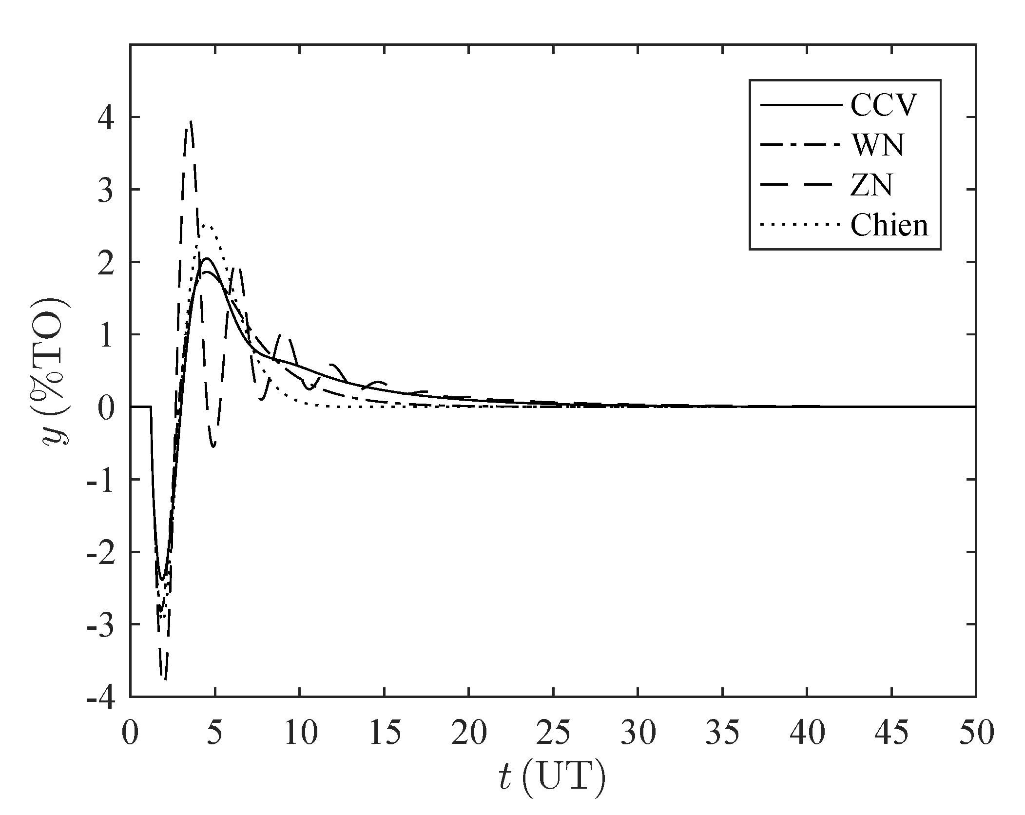
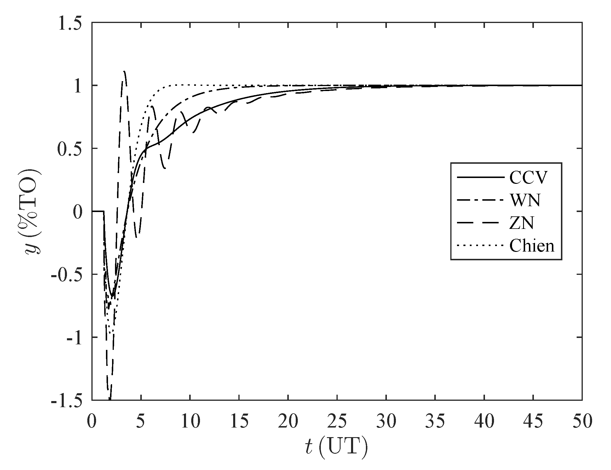
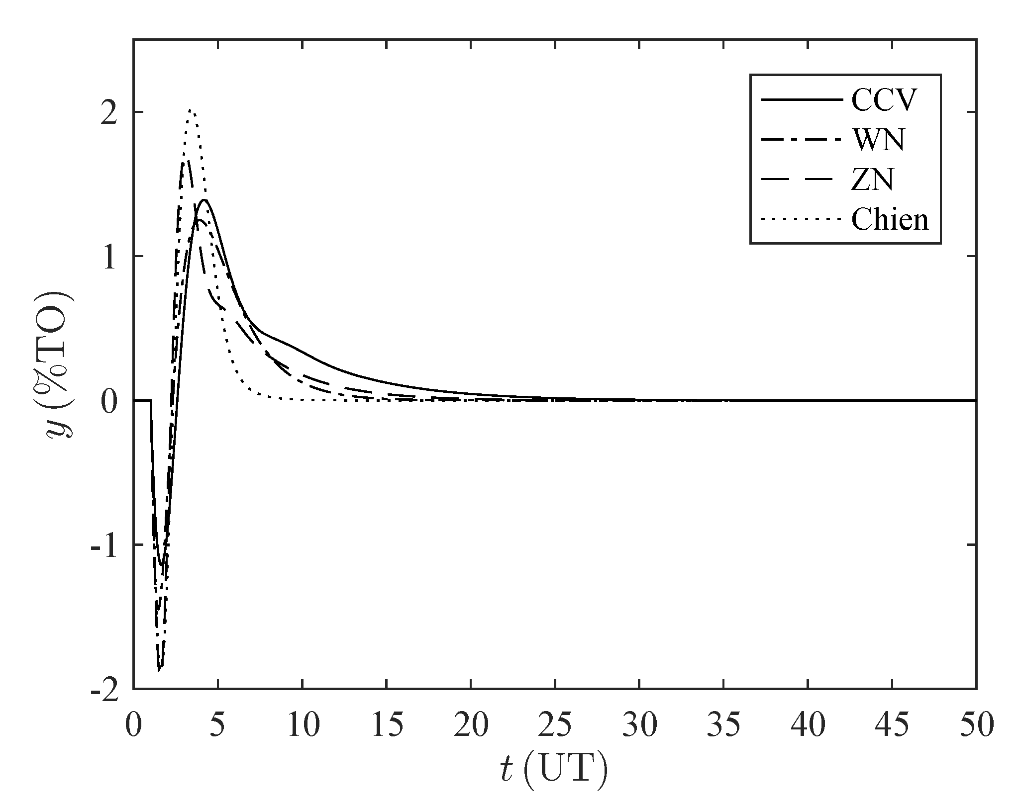
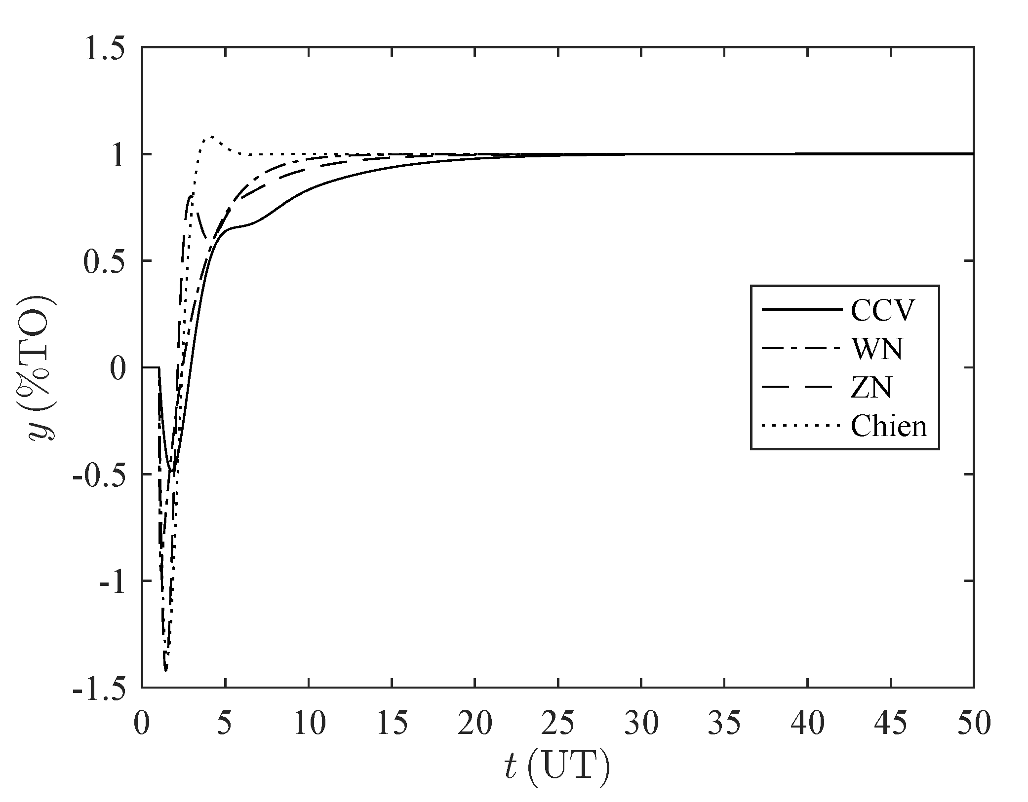
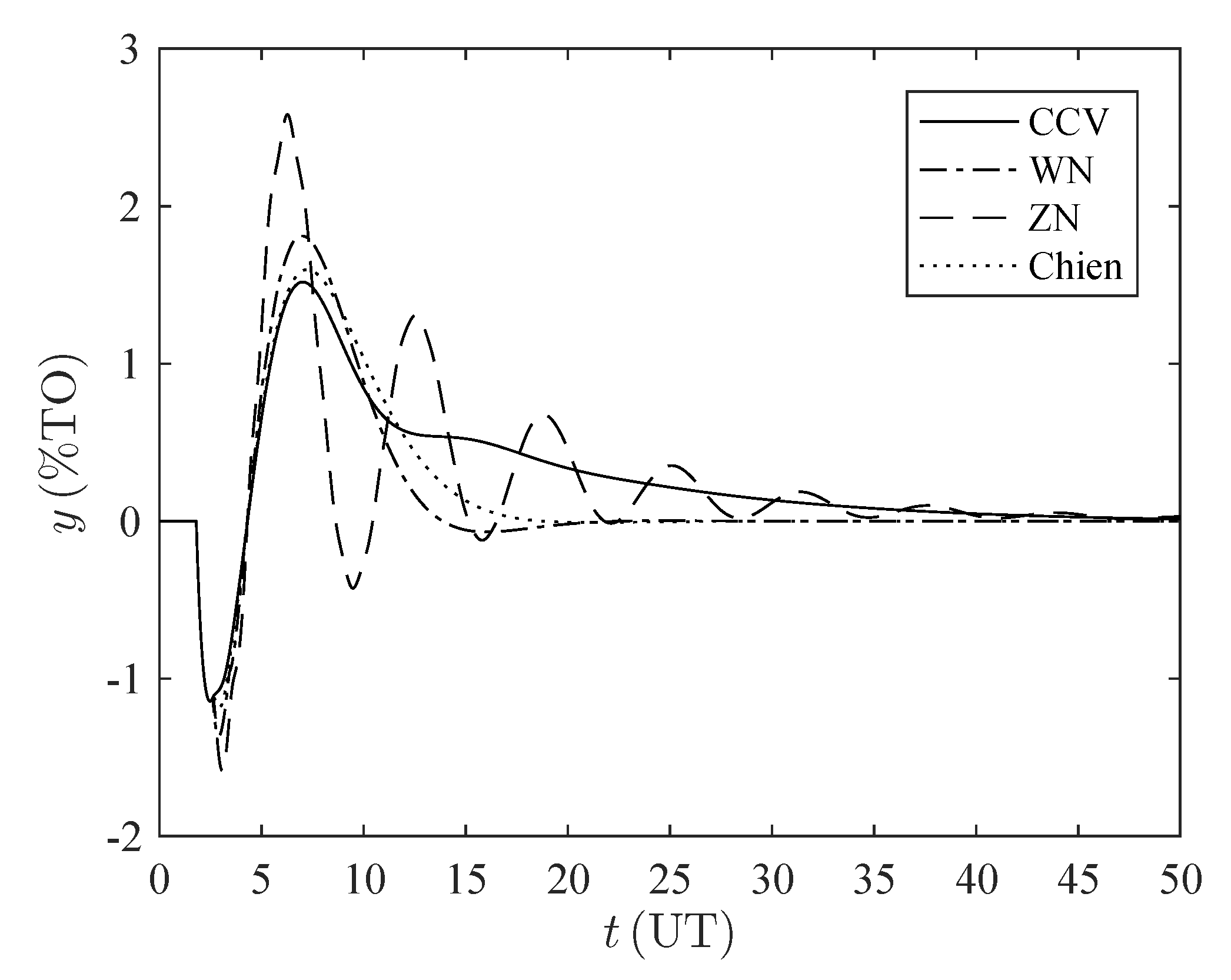
Figure 5 and Figure 6 show the time response for the parameter set $P_4$, for both disturbance rejection and set-point tracking, respectively.

It can be noticed that the CCV controller has a high settling time; this occurs because of the high value assigned to the suppression factor ($\gamma =4$), in order to penalize the manipulated variable and increase the robustness, smooths the actuator’s behavior. Additionally, it can be noticed how the CCV controller decreases the inverse response effect.

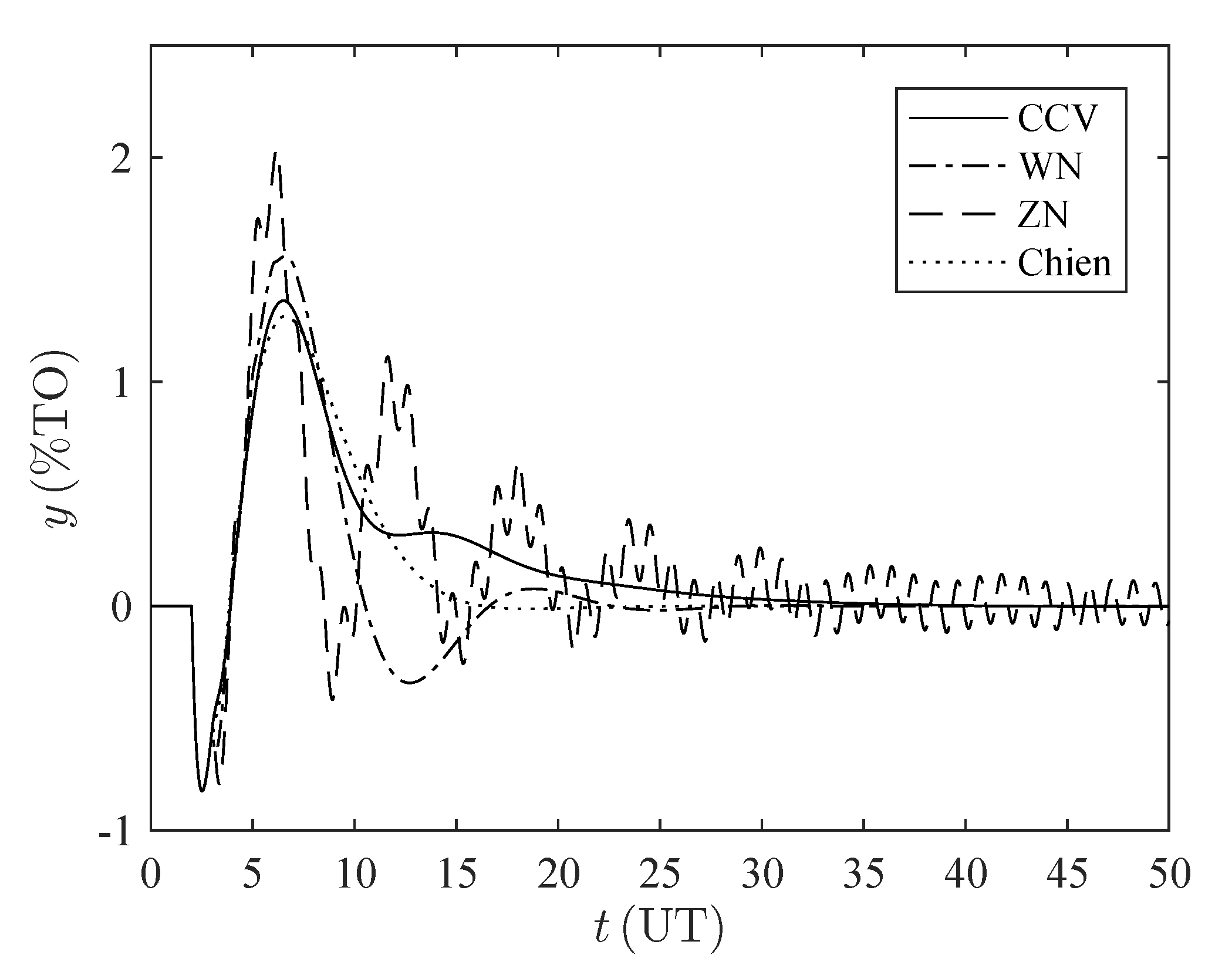
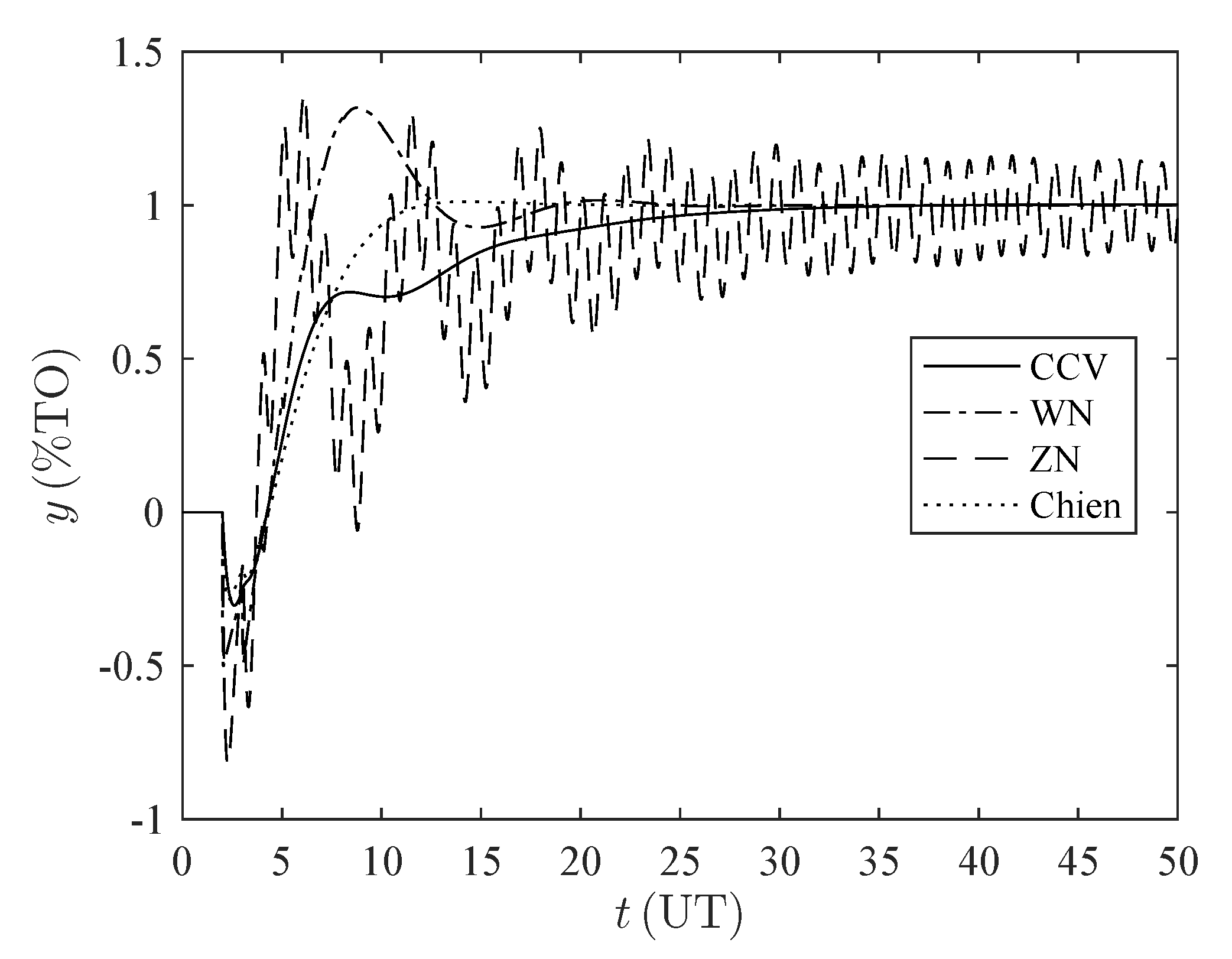
This procedure was followed for the other parameter sets. In Appendix B,

Table A2. Performance indexes. Disturbance rejection for the set $P_1$.

Method	$\mathit{ISE}{}^{\mathit{a}}$	$\mathit{IAE}{}^{\mathit{b}}$	$\mathit{IMV}{}^{\mathit{c}}$	$\mathit{MP}{}^{\mathit{d}}$
CCV	16.7200	13.6500	2.3560	2.0500
WN	17.2200	11.9800	2.9170	1.8622
ZN	30.9500	16.1800	8.2430	3.9959
CCCC	22.4200	11.6200	2.9820	2.5230

${}^a{(\%\mathrm{TO})}^2·\mathrm{UT}$; ${}^b\%\mathrm{TO}·\mathrm{UT}$; ${}^c\%\mathrm{CO}$; ${}^d\%\mathrm{TO}$.

,

Table A3. Performance indexes. Set-point tracking for the set $P_1$.

Method	$\mathit{ISE}{}^{\mathit{a}}$	$\mathit{IAE}{}^{\mathit{b}}$	$\mathit{IMV}{}^{\mathit{c}}$	$\mathit{MP}{}^{\mathit{d}}$
CCV	6.9980	8.1680	0.7902	1.0007
WN	6.7140	6.4190	7.2390	1.0000
ZN	8.7490	8.5640	4.1430	1.3683
CCCC	7.3370	5.2440	3.6010	1.0039

${}^a{(\%\mathrm{TO})}^2·\mathrm{UT}$; ${}^b\%\mathrm{TO}·\mathrm{UT}$; ${}^c\%\mathrm{CO}$; ${}^d\%\mathrm{TO}$.

,

Table A4. Performance indexes. Disturbance rejection for the set $P_2$.

Method	$\mathit{ISE}{}^{\mathit{a}}$	$\mathit{IAE}{}^{\mathit{b}}$	$\mathit{IMV}{}^{\mathit{c}}$	$\mathit{MP}{}^{\mathit{d}}$
CCV	6.3040	8.2120	1.9840	1.3950
WN	5.6930	6.4080	2.8620	1.2494
ZN	6.9180	7.0620	4.3250	1.7070
CCCC	8.5510	5.9770	4.0270	2.0238

${}^a{(\%\mathrm{TO})}^2·\mathrm{UT}$; ${}^b\%\mathrm{TO}·\mathrm{UT}$; ${}^c\%\mathrm{CO}$; ${}^d\%\mathrm{TO}$.

,

Table A5. Performance indexes. Set-point tracking for the set $P_2$.

Method	$\mathit{ISE}{}^{\mathit{a}}$	$\mathit{IAE}{}^{\mathit{b}}$	$\mathit{IMV}{}^{\mathit{c}}$	$\mathit{MP}{}^{\mathit{d}}$
CCV	4.5670	5.9050	0.7466	1.0010
WN	4.1240	4.1000	12.8100	1.0001
ZN	4.8090	4.1760	1.9400	1.0000
CCCC	5.2480	3.0810	0.8966	1.0822

${}^a{(\%\mathrm{TO})}^2·\mathrm{UT}$; ${}^b\%\mathrm{TO}·\mathrm{UT}$; ${}^c\%\mathrm{CO}$; ${}^d\%\mathrm{TO}$.

,

Table A6. Performance indexes. Disturbance rejection for the set $P_3$.

Method	$\mathit{ISE}{}^{\mathit{a}}$	$\mathit{IAE}{}^{\mathit{b}}$	$\mathit{IMV}{}^{\mathit{c}}$	$\mathit{MP}{}^{\mathit{d}}$
CCV	7.5120	10.2800	1.6450	1.3635
WN	8.4030	8.8060	3.8160	1.5593
ZN	10.8800	13.1600	38.0600	2.0353
CCCC	7.2170	8.1150	1.6610	1.2914

${}^a{(\%\mathrm{TO})}^2·\mathrm{UT}$; ${}^b\%\mathrm{TO}·\mathrm{UT}$; ${}^c\%\mathrm{CO}$; ${}^d\%\mathrm{TO}$.

,

Table A7. Performance indexes. Set-point tracking for the set $P_3$.

Method	$\mathit{ISE}{}^{\mathit{a}}$	$\mathit{IAE}{}^{\mathit{b}}$	$\mathit{IMV}{}^{\mathit{c}}$	$\mathit{MP}{}^{\mathit{d}}$
CCV	6.0110	8.4260	0.7220	1.0031
WN	5.8830	6.5500	21.0900	1.3184
ZN	8.0590	12.2700	58.0600	1.3625
CCCC	5.6740	6.2400	1.2470	1.0119

${}^a{(\%\mathrm{TO})}^2·\mathrm{UT}$; ${}^b\%\mathrm{TO}·\mathrm{UT}$; ${}^c\%\mathrm{CO}$; ${}^d\%\mathrm{TO}$.

,

Table A8. Performance indexes. Disturbance rejection for the set $P_5$.

Method	$\mathit{ISE}{}^{\mathit{a}}$	$\mathit{IAE}{}^{\mathit{b}}$	$\mathit{IMV}{}^{\mathit{c}}$	$\mathit{MP}{}^{\mathit{d}}$
CCV	13.1300	16.7700	1.6610	1.5205
WN	14.2600	11.4000	3.2050	1.8102
ZN	20.9300	17.6900	7.8383	2.5812
CCCC	12.5000	13.5400	1.4470	1.5975

${}^a{(\%\mathrm{TO})}^2·\mathrm{UT}$; ${}^b\%\mathrm{TO}·\mathrm{UT}$; ${}^c\%\mathrm{CO}$; ${}^d\%\mathrm{TO}$.

and

Table A9. Performance indexes. Set-point tracking for the set $P_5$.

Method	$\mathit{ISE}{}^{\mathit{a}}$	$\mathit{IAE}{}^{\mathit{b}}$	$\mathit{IMV}{}^{\mathit{c}}$	$\mathit{MP}{}^{\mathit{d}}$
CCV	8.9170	13.0100	0.7630	0.9951
WN	7.6430	6.9760	19.3000	1.0624
ZN	9.8820	11.7200	7.1650	1.1496
CCCC	7.6740	7.6310	2.5230	1.0080

${}^a{(\%\mathrm{TO})}^2·\mathrm{UT}$; ${}^b\%\mathrm{TO}·\mathrm{UT}$; ${}^c\%\mathrm{CO}$; ${}^d\%\mathrm{TO}$.

contain the performance indexes for disturbance rejection and set-point tracking for the remaining sets of the parameters $P_1$, $P_2$, $P_3$, and $P_5$. In Appendix C, Figure A1, Figure A2, Figure A3, Figure A4, Figure A5, Figure A6, Figure A7 and Figure A8 show the time response for the remaining sets of parameters: $P_1$, $P_2$, $P_3$, and $P_5$.

All the points obtained by each tuning method using the scoring system were added, by considering each performance index.

Table 9. Total scores for disturbance rejection for the set $P_4$.

Method	$\mathit{ISE}$	$\mathit{IAE}$	$\mathit{IMV}$	$\mathit{MP}$	Total
CCV	17	9	19	17	62
WN	14	16	12	15	57
ZN	6	6	5	6	23
CCCC	13	19	14	12	58

All units are points.

shows the total scores for disturbance rejection and

Table 10. Total scores for set-point tracking for the set $P_4$.

Method	$\mathit{ISE}$	$\mathit{IAE}$	$\mathit{IMV}$	$\mathit{MP}$	Total
CCV	12	8	20	17	57
WN	19	16	6	14	55
ZN	6	7	9	8	30
CCCC	13	19	15	11	58

All units are points.

shows the total scores for set-point tracking.

As it can be noticed, the proposed CCV method shows the best over-all results for disturbance rejection, when considering a wide range of parameters of the process’ transfer function. Although the controller was tuned for disturbance rejection, it still offers a very good performance for set-point tracking, when considering the same wide range of parameters of the process’ transfer function. In both operations (servo and regulatory), the CCV method achieves the best performance in both the $MP$ and $IMV$ indexes, which indicates that this tuning method benefits the durability of the actuator.

Although IMC is based on a pole-zero cancellation, which can lead to poor performance in the load regulation operation [65] for lag-dominant processes [66], in Appendix D we provide another simulation for a set of parameters with small dead time and high time constant ($\eta =0.1$, $\theta =0.01$, ${\tau }_2=0.9$, ${\tau }_1=1$) that shows the wide application of the CCV method; this set is in the limits of the experimental region, but that was not given within the sets selected by the experimental design.

6. Discussion on Robustness Analysis

Romagnoli and Palazoglu [6] stated that there are different techniques to evaluate uncertainties in a control system. One of them consists in the selection of a range of the parameters of the process’ transfer function, as in [67], in which Arbogast et al. proposed a robust stability factor metric to examine the effect of plant-model mismatch in the process gain, dead time, and time constant for self-regulating processes. Such method uses the relation of the values of parameters that bring the system’s response to marginally stable conditions and the values of the parameters used for tuning.

Following such technique, in this work the robustness analysis consists on the study of the variability of parameters $\widehat{\eta }$ and $\widehat{\theta }$ from Table 3 by considering a value for the suppression factor $\gamma =4$. The analysis was done using a Simulink scenario in which small increments for the parameter of interest were done while keeping constant all the other parameters in the plant and the controller. Simulations stopped when the output reached a sustained-oscillation response (marginal stability conditions), hence, the ultimate value was found for each parameter. Results are found in

Table 11. Robustness for sets $P_1$, $P_2$, $P_3$, $P_4$, $P_5$.

Method	Set ${\mathit{P}}_1$		Set ${\mathit{P}}_2$		Set ${\mathit{P}}_3$		Set ${\mathit{P}}_4$		Set ${\mathit{P}}_5$
	$\widehat{\mathit{\eta }}$	$\widehat{\mathit{\theta }}$	$\widehat{\mathit{\eta }}$	$\widehat{\mathit{\theta }}$	$\widehat{\mathit{\eta }}$	$\widehat{\mathit{\theta }}$	$\widehat{\mathit{\eta }}$	$\widehat{\mathit{\theta }}$	$\widehat{\mathit{\eta }}$	$\widehat{\mathit{\theta }}$
CCV	5.9710	9.0310	3.8950	6.8300	5.3140	11.6650	8.7890	16.6050	8.2950	18.0600
WN	6.3060	5.8040	4.0000	3.6900	3.5860	3.6900	7.7520	7.2350	6.0180	5.8100
ZN	3.8050	0.7400	2.7560	3.8000	2.0930	1.0460	4.8640	1.1530	4.0550	1.7000
CCCC	5.0950	3.6720	5.5650	7.0000	5.5590	7.0000	7.3040	6.4480	7.0650	7.5700

. The table indicates the value of the parameter that leads the response to reach sustained oscillations for each controller and for a particular set of parameters. Therefore, the higher the ultimate value the more robust is the technique with respect to changes in the parameter that is being analyzed.

The CCV controller is more robust with respect to variations in $\widehat{\theta }$, specially in the case when the dominant time constant and dead time are almost equal, or even equal. The ratio between dead time and the dominant time constant $\widehat{\theta }=\frac{\theta }{{\tau }_1}$, is known as the uncontrollability parameter and when it is near 1, it is more difficult to control the process [68]. Therefore, the CCV tuning method becomes a technique suitable for high values of such parameter. On the contrary, for low values of $\widehat{\theta }$, the CCV controller does not achieve the better results. With respect to $\widehat{\eta }$, the CCV and CCCC controllers are more robust; both with similar results. However, the latter gets better results for low values of $\widehat{\theta }$.

7. Conclusions

In this work, we proposed an IMC-based PID tuning method for inverse-response second-order plus dead time systems. The tuning rules are based on the optimization of an objective function that combines performance and robustness. The tuning method has been presented by using an easy-to-follow ten-step methodology with equations that are mathematically simple.

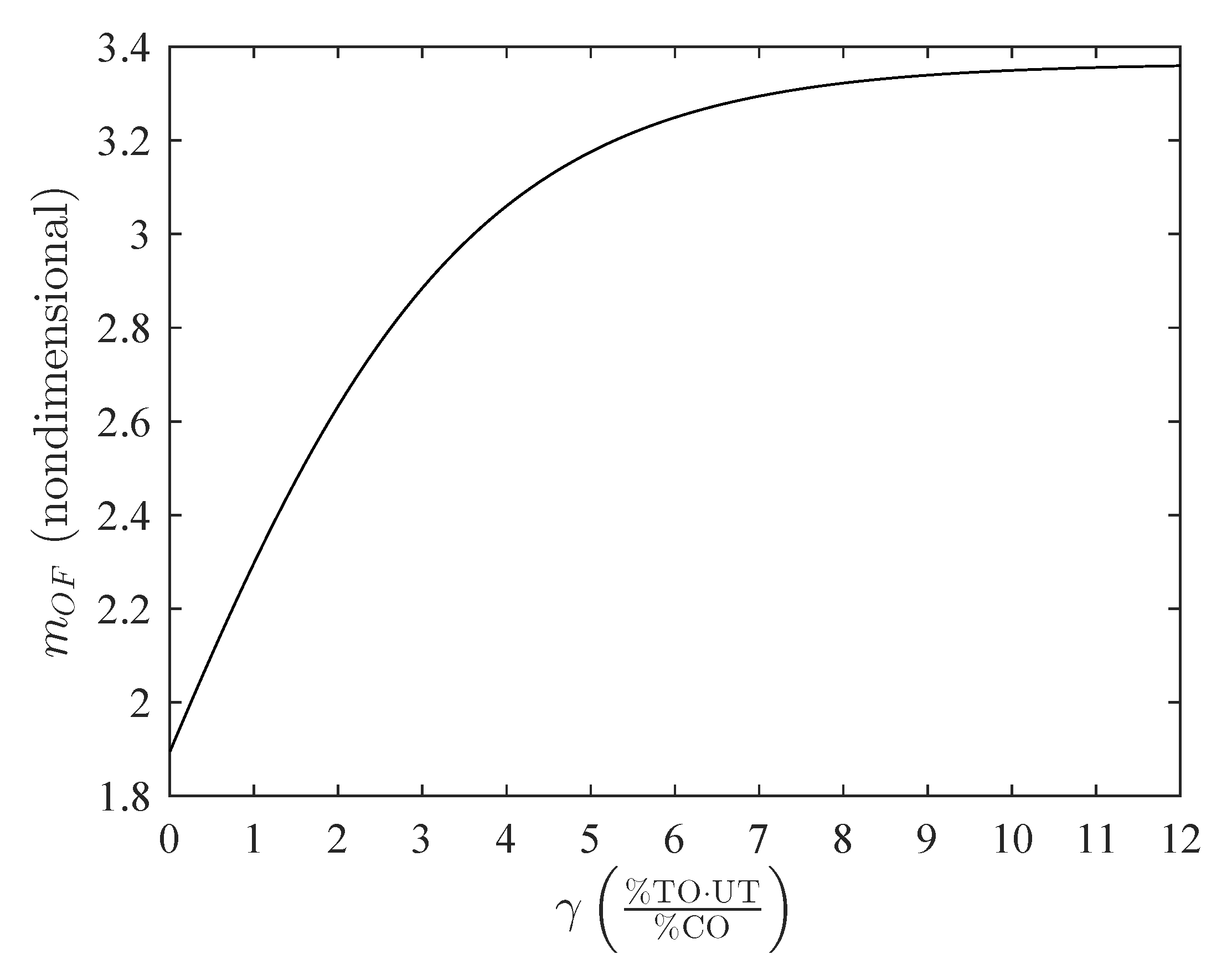
A correlation that allows one to compute the value of the tuning parameter ${\tau }_c$ that minimizes the objective function has been found. The tuning parameter ${\tau }_c$, affects the stability of the closed-loop control system. Small values of ${\tau }_c$ increase the speed response of the system, but also produce an oscillatory response, to the point that the system can become unstable. Nondimensionalization reduced the number of parameters, which allows the reduction of simulations runs, saving computation time. The central composite experimental design allowed the authors to determine the appropriate number of simulations, and obtain goodness of fit for the proposed model.

The performance of a PID controller, tuned with the proposed CCV and other literature-existing tuning rules, was evaluated. The performance achieved with the proposed CCV method was excellent, not only for disturbance rejection but for set-point tracking, when considering a wide-range of parameters of the process’ transfer function. For both operations (servo and regulatory), the CCV method achieves the best performance in both the MP and IMV indexes, which indicates that this tuning method benefits the durability of the actuator. This is a very important result regarding continuous plant operation in industrial processes, since it can help avoiding unexpected plant stops caused by actuator failures.