Abstract
When exposed to viscous heating, hydraulic valve orifices experience thermal deformation, which causes spool clamping and actuator disorder. Quantitative research on thermal deformation can help reveal the micro-mechanism of spool clamping. In this study, miniature thermocouples are embedded into a valve orifice with an opening size of 1 mm to measure temperature distribution. An optimization algorithm based on measurement data (M-OA) for the thermal deformation of the valve orifice is proposed. The temperature and thermal deformation of the valve orifice are calculated through Fluent and Workbench joint simulation, with the measurement data serving as boundary conditions. Results show that, for a valve orifice with a valve wall length of 18 mm, when the temperature of the sharp edge is at 60 °C, thermal deformation measures 7.7 μm via observation and 7.62803 μm via M-OA, indicating that the M-OA method is reliable. The results of the joint simulation can be accepted because measurements of temperature reached an accuracy rate of 95%, and that of deformation reached 82.7%. A large drop in pressure led to a rapid increase in temperature, causing serious thermal deformation of the valve orifice. With an inlet pressure of 3 MPa, the temperature of the sharp edge reached 72.9 °C within 110 min, and radial thermal deformation can reach 8.3 μm. Such deformation poses great risk of spool clamping for a spool valve of Φ36 mm.
1. Introduction
Hydraulic systems control the motions of actuators via hydraulic valves. Spool valves, the most widely used type, exert a strong impact on the stability of actuators, and spool clamping leads directly to actuator disorder and even safety-related accidents. Spool clamping is caused by two main factors: unexpected forces generated at macro level, such as flow force [1,2,3,4,5], and deterioration of lubrication clearance generated at micro level. The size of a clearance should be set with regard to the following: the clearance should be small enough to prevent internal leakage, yet big enough to provide the sufficient space needed to ensure smooth action [6,7]. Barriers to achieving ideal clearance include factors such as roughness variation [8,9,10,11], particle pollution [12,13,14,15,16,17] and thermal deformation of valve orifices. Thermal deformation occurs when viscous heating generated by fluids increases the temperature of the valve orifice.
Updating hydraulic technology requires hydraulic components of high quality; however, spool clamping caused by thermal deformation of valve orifices has not been studied comprehensively, and only a few scholars have done such research. Shao Xueming simulated spool deformation by using the fluid–structure interaction method in ABAQUS software and studied two valve spools damaged by jamming [18] (ABAQUS is a powerful set of engineering simulation finite element software that solves problems ranging from relatively simple linear analysis to many complex nonlinear problems. Which was produced by Dassau SIMULIA Corporation, and headquartered in Providence, Rhode Island, USA.). Ji Hong studied the influence of the throttle groove number on valve spool thermal deformation by using ANSYS, found that the maximum deformation in the spool and valve body caused by a rise in temperature can reach several microns; overall bending deformation in the spool and valve body was also observed. Such deformation can directly lead to spool clamping [19,20] (The headquarters of ANSYS company is located in the Pittsburgh in Granonsburg, Pennsylvania, USA. ANSYS software is a large-scale and general finite element analysis (FEA) software, and the fastest growing Computer-Aided Engineering (CAE) software in the world.). S.V. Angadi studied a multi-physics model that includes the coupled effects of electromagnetics, thermodynamics and solid mechanics. The resulting finite element model of the solenoid valve revealed the failure mechanism and its relation to temperature distribution, mechanical and thermal deformations and stresses [21,22]. Zhao Jianhua numerically simulated heat–fluid–solid coupling by using the finite element method and solved the problem of degraded control accuracy and clamping stagnation of servo valves in situations with large temperature differences. The distribution rules of the temperature and thermal deformation of the shell, spool and valve sleeve and the pressure, velocity and temperature field of the flow channel were also analyzed [23]. Jin He confirmed that the quasi-stationary state exists in the 3D valve body warm-up process [24]. Maher A.R. Sadiq Al-Baghdadi investigated mechanical and thermal stresses that arise in the exhaust valve due to the valve’s operation with and without a thermal coating layer (ceramic) on its surface [25]. Bo Wu designed a new type of exhaust valve, simulated its thermal deformation field by using ANSYS, and compared the obtained thermal deformation field with that of a traditional exhaust valve [26]. Zhou Jialing heated a cylindrical sample of ϕ 8 mm × 15 mm at a heating rate of 10 °C/s and kept the temperature at 950 °C for 5 min once it was reached; then, the sample was cooled to 450–650 °C at a cooling rate of 10 °C/s and finally tested with a Gleeble-1500 thermal simulation machine, getting the maximum thermal deformation of 0.70 mm [27]. In addition, several studies focused on the coefficient of thermal expansion (CTE) and its relationship with the thermal deformation of certain materials [28,29,30,31,32,33]. These studies showed that CTE changes with temperature. Therefore, it is evident that uneven temperatures and CTE should not be ignored in the calculation of the thermal deformation of hydraulic valve orifices.
In accordance with these studies, in this paper, the micro-mechanism of spool clamping caused by thermal deformation of the valve orifice is deduced and presented in Figure 1.
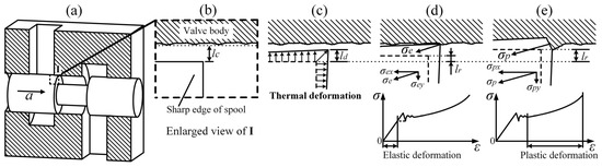
Figure 1.
Micro-mechanism of spool clamping caused by thermal deformation of the valve orifice: (a) The standard structure of a spool valve; (b) Enlarged micron-level view of valve orifice; (c) Radial thermal deformation ld; (d) Spool clamping caused by small radial fretting allowance lr; (e) Spool clamping caused by large radial fretting allowance lr.
Figure 1a shows the standard structure of a spool valve, mainly comprising the valve body and spool. The spool moves along the valve hole at an acceleration of ‘a’ m2/s (the value of ‘a’ can be 0 m2/s). The valve opening undergoes positive, zero and negative opening stages. An enlarged micron-level view of valve orifice when the sharp edge of the spool has slid into the valve hole is shown in Figure 1b. Ideally, a certain clearance lc exists between the valve hole and spool; in this study, it is called ‘unilateral clearance’ of the spool valve, and it allows the lubricating oil to fully fill the clearance, ensuring that the spool moves smoothly. However, in reality, before the spool slides into the valve hole, it works under hydraulic pressure for a certain period of time, inevitably generating thermal deformation and radial thermal deformation ld, as shown in Figure 1c, reducing the radial fretting allowance. Making the spool absolutely collinear with the valve hole is difficult at the micron level, and radial fretting allowance lr is generated. As indicated in Figure 1d, when lr = lc − ld, the sharp edge of the spool comes into contact with the wall of the valve hole. Given that the surface of the valve hole wall is rough, elastic stress σe is generated; it increases linearly with elastic deformation ε and resolves small component force σex along the medial axis of the valve hole, thereby impeding the action of the spool. Figure 1e shows that when lc − ld < lr < lc, the sharp edge of the spool jams into the wall of the valve hole and subsequently generates plastic stress σd. σd increases exponentially with plastic deformation ε and resolves large component force σpx along the medial axis of the valve hole, thereby causing spool clamping.
The preceding analysis indicates that spool clamping is considerably affected by the relationships between unilateral clearance lc, radial fretting allowance lr and radial thermal deformation ld. lc and lr are determined by the processing technology and assembly process, and calculations of ld must consider complex working conditions, which is crucial in determining the risk of spool clamping and must be calculated accurately.
In this study, a cylindrical spool valve orifice is converted into a simpler planar valve orifice, and miniature thermocouples are embedded in the simplified valve orifice to determine temperature distribution. An optimization algorithm based on the measurement temperature (M-OA) is then proposed, and thermal deformation is calculated using self-developed software. Thermal deformation of the valve orifice is observed with a microscope and used to demonstrate the accuracy of the M-OA method. A Fluent and Workbench joint simulation is performed to simulate the temperature and thermal deformation of the valve orifice, and the measured inlet and outlet temperature data serve as the boundary conditions. On the basis of the M-OA and simulation results, thermal deformation of the valve orifice is presented quantitatively, and the micro-mechanism of spool clamping caused by thermal deformation of the valve orifice is demonstrated.
2. Design of the Experimental Device
The experimental model is comprised of two parallel valve orifices. One is the temperature measurement valve orifice, formed by a part for measuring temperature (Figure 2a), and assembly parts for the valve orifice (Figure 2c); the other is the micro observation valve orifice, formed by the micro observation part (Figure 2b) and valve orifice assembly part. The valve opening measured 1 mm, the vertical edge of part 1 and part 2 measured 18 mm, and all the parts were made of # 45 steel.
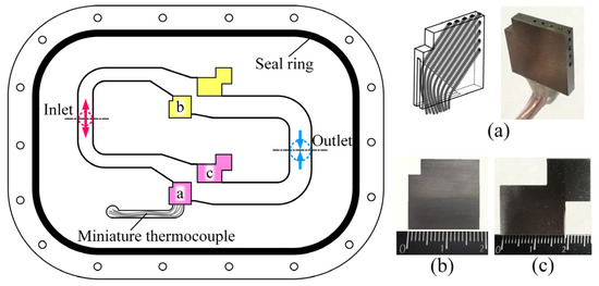
Figure 2.
Parallel valve orifice experimental model: (a) Temperature measurement part; (b) Micro observation part; (c) Valve orifice assembly part.
In accordance with the valve orifice experimental model, a device was designed to collect temperature data and an image of the deformation of the valve orifice. Figure 3 shows a 3D diagram of said device. It includes a support frame made by 3D printing, and the longitude slideway, the latitude slideway and the height adjustment screw are used to adjust the position of the observation platform of the microscope.
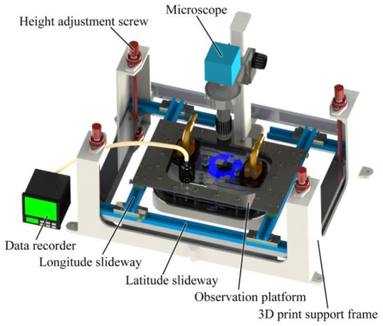
Figure 3.
Valve orifice temperature measurement device.
The device was connected to the hydraulic system, as shown in Figure 4. The hydraulic pumping station (1) provided oil for the experiment. The oil filter (3), throttle valve (4), inlet pressure gauge (5) and inlet thermometer (6) (used to test the inlet temperature of CH10) are integrated into the inlet integration block (8). The outlet pressure (9) gauge and outlet thermometer (10) (used to test the device outlet temperature of CH11) are integrated into the outlet integration block. The flow gauge (11) and data recorder (14) are also accessed through this system.
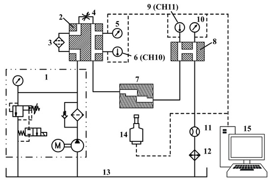
Figure 4.
Hydraulic system used in the experiment: 1—hydraulic pumping station; 2—inlet integration block; 3—oil filter; 4—throttle valve; 5—inlet pressure sensor; 6—inlet thermometer; 7—experimental device; 8—outlet integration block; 9—outlet thermometer; 10—outlet pressure sensor; 11—flowmeter; 12—radiator; 13—hydraulic tank; 14—microscope; 15—data recorder.
The actual platform used in the experiment is shown in Figure 5. A miniature Type T thermocouple with a measuring range of 0–150 °C was used, the measurement accuracy of which is ±0.5 °C. The microscope has an observation accuracy of 1 μm and an assessment precision of 0.1 μm. The pressure-resistant range is 0–3.5 MPa. The technical features of the platform are as follows: Measurement of the temperature distribution of valve orifice in real time, synchronous observation of the thermal deformation, use of 3D printing technology in building adjustable support device. Additionally, HM46 hydraulic oil was used as the fluid oil, and the inlet pressure of the device was adjusted using the relief valve. Because the oil in an open oil tank is exposed to the atmosphere, the outlet pressure is roughly the same as that of atmospheric pressure, meaning that the inlet pressure can be used to represent the pressure drop in the valve orifice.
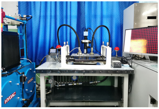
Figure 5.
Platform used in experiment for valve orifice temperature measurement.
3. Analysis of Experiment Results
3.1. Analysis of Temperature Measurement Results under Different Pressure Drops
Three separate experiments are conducted, with conditions being a valve opening of 1 mm and inlet pressures of 1 MPa, 2 MPa and 3 MPa. The results are shown in Figure 6. Figure 6a presents the measurement locations of the miniature thermocouples. Four measurement probes from CH1 to CH4 are embedded in the horizontal valve wall, and four measurement probes from CH6 to CH9 are embedded in the vertical valve wall; the sharp edge is measured using CH5. In addition, the temperature of the oil tank is used as reference of the temperature of the valve orifice.
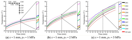
Figure 6.
Temperature curves of the valve orifice with different pressures in the experiment.
Figure 6 indicates that the temperatures of the different locations increased gradually and synchronously with time and were distributed in layers. The curves at 60 min were enlarged within a small temperature range because these curves crowded together under a large temperature range. Comparison of Figure 6a–c shows that when inlet pressures were at 1 MPa, 2 MPa and 3 MPa, the temperatures of the sharp edge (CH5) became 41.9 °C, 52.8 °C and 61.4 °C, respectively. This result means that there is a strong positive correlation between the heating rate of the valve orifice and the drop in pressure. Given T0(t) as the reference temperature of the oil tank, T1(t) is the temperature of the sharp edge (CH5), and is the time-average value of T1(t) − T0(t). Upon calculation, we can see that when pin = 1 MPa, ≈ 5.8 °C; when pin = 2 MPa, ≈ 8.5 °C; when pin = 1 MPa, ≈ 14.6 °C. This indicates that the higher the pressure drop, the higher the local temperature of the sharp edge.
3.2. Characteristics of the Temperature Distribution in the Valve Orifice
Radar charts are created every 10 min in accordance with the curves in Figure 6b to illustrate intuitively the temperature distribution and change in the valve orifice. These charts are shown in Figure 7.
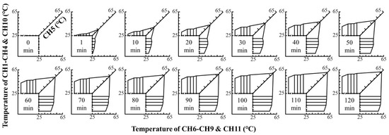
Figure 7.
Temperature change in the valve orifice at different times when x = 1 mm and pin = 2 MPa.
Figure 7 indicates that the temperature of the valve orifice increased with time. The temperature in the sharp edge (CH5) is higher than that of other places; it increased from 35.6 °C to 62 °C in the timeframe of the experiment. The temperature of the other measurement points decreased as the distance to the sharp edge (CH5) increased. The curves of CH6, CH7 and CH8 were higher than those of CH1, CH2 and CH3. In other words, the temperature of the vertical wall was higher than that of the horizontal wall because the oil’s temperature increased after it passed through the valve orifice.
3.3. Analysis of Thermal Deformation Observation Results
A microscope was used to capture images of the micro thermal deformation of the valve orifice as the temperature increased. These images are presented in Figure 8.
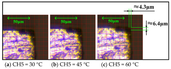
Figure 8.
Micro thermal deformation images of the sharp edge as temperatures rose.
Figure 8 indicates that as the temperature of the sharp edge increased from 30 °C to 60 °C, the deformation in the horizontal and vertical directions was approximately 4.3 μm and 6.4 μm, respectively. The sum of the squares of deformation in both the horizontal and vertical directions was calculated, and the root was determined to obtain the deformation of the sharp edge (~7.7 μm). The observation result can be perceived directly but is lacking in accuracy; hence, the value of thermal deformation needs to be further quantified.
3.4. Optimal Algorithm of Thermal Deformation Based on Measured Temperature Data
On the basis of the discrete temperature data of the valve wall, an optimal algorithm was applied to calculate the thermal deformation of valve orifice. The point opposite the sharp edge of the valve orifice was used as the origin. The endpoint of the sharp edge was projected on the x and y axes, and the lengths of the projection were expressed as lx and ly. The horizontal and vertical valve walls were located on the x and y axes, respectively, and f(x) and g(y) were assumed to be continuous temperature functions on the x and y axes, respectively. Ut represented the maximum deformation of the valve orifice. The calculation principle of the M-OA method is shown in Figure 9, which also presents the process of the optimal algorithm in detail. After acquiring discrete temperature data from CH1 to CH9, the data from CH1 to CH5 were fitted as f(x), and the data from CH5 to CH9 were fitted as g(y), as indicated in Figure 10.
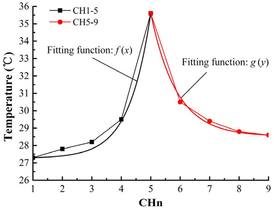
Figure 9.
Thermal deformation calculation principle of valve orifice in the optimization algorithm based on measurement data (M-OA) method.
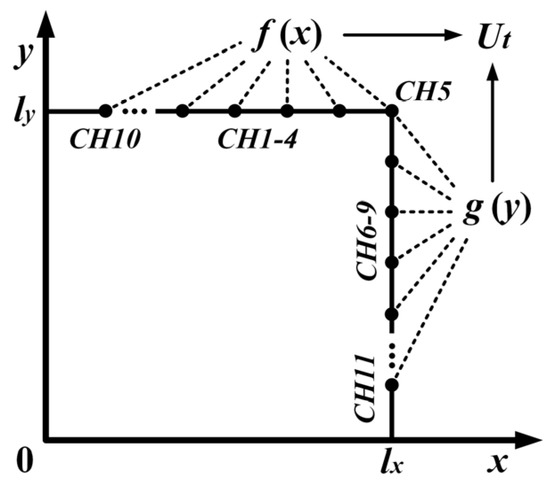
Figure 10.
Fitted wall temperature curves based on measurement data.
Continuous temperature functions f(x) and g(y) were fitted to higher-order functions, as presented in Equation (1).
The thermal deformation of the valve orifice was calculated based on the fitted temperature functions f(x) and g(y). The optimal algorithm of thermal deformation was derived from the empirical thermal deformation equation of solids, which is expressed as
where ∆l is the solid deformation caused by the temperature rise, l is the original size of the measured object, α is the CTE of a certain material and T0 is the initial temperature of the object (after a period of temperature rise, the temperature of the object reaches T). In Equation (2), α is assumed to be constant within a large temperature range, and the temperature distribution is proven to be uneven by the measurement above; the value of α also changes continuously with temperature [34,35].
Given α(x) and α(y) as functions of CTE on the x and y axes, which change with f(x) and g(y), Equation (3) was established as
where the functions of α(x) and α(y) contain coefficients α0 and β; α0 is the basic term of the optimal CTE, and β is the correction factor derived from engineering experience [36].
Equations (1) and (3) were inputted into Equation (2), and their new functions were integrated into the x and y axes, respectively. Subsequently, the thermal deformation on the x and y axes was derived as Ux and Uy, respectively, which can be expressed as follows:
The maximum thermal deformation of the valve orifice can be expressed as
For convenience in calculation, a computer program and application interface were built in accordance with the optimal algorithm, as shown in Figure 11. Users only need to input the measurement temperature data of the valve orifice, the coefficient α0 and the parameters lx, ly and T0; then, the temperature distribution curves of the valve wall will be given, and the maximum thermal deformation will be outputted immediately.
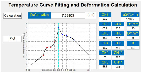
Figure 11.
Application interface of the M-OA method (x = 1 mm, pin = 2 MPa, t = 105 min, CH1-9).
As shown in Figure 11, the data were measured under the conditions of x = 1 mm and pin = 2 MPa and at the moment of 105 min when the sharp edge (CH5) had just reached 60 °C. α0 = 1.16 × 10⁻⁵/°C and β = 8.58 × 10⁻⁹/°C because the material of the valve orifice was # 45 steel. The feature size of the planar valve core was lx = ly = 18 mm, and the initial temperature of the valve orifice (T0) was equal to 27.3 °C. The fitted curve indicates that, as the measurement point changed, the temperature of the horizontal valve wall (CH1 to CH4) increased sharply and reached its peak at point CH5; afterward, it decreased slowly along the vertical valve wall (CH6 to CH9). The inlet (CH10) and outlet (CH11) data were adopted as supplementary data because the measurement points were limited. Notably, additional measurement points can be arranged to enhance the resolution of the temperature curve. The thermal deformation was determined to be 7.62803 μm, which is close to the observation result obtained when the temperature was 60 °C (7.7 μm) (Figure 8).
The thermal deformations of the valve orifice under inlet pressures of 1 MPa, 2 MPa and 3 MPa and at 120 min were calculated with the M-OA method, as indicated in Figure 12.
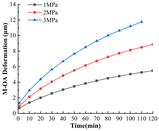
Figure 12.
Thermal deformations of the valve orifice calculated with the M-OA method with Pin = 1 MPa, 2 MPa and 3 MPa.
As indicated in Figure 12, the thermal deformation curves increased gradually with time, and the higher the inlet pressure was, the faster the deformation increased. For example, at 60 min, the deformation under the inlet pressures of 1 MPa, 2 MPa and 3 MPa was 3.85 μm, 6.71 μm and 8.5 μm, respectively. The growth rate of all the curves approached 0 μm/min due to heat exchange and thermal stress of the material. This result indicates that, at a certain moment, the thermal deformation of the valve orifice ceased to increase and reached peak value. This particular moment poses the highest risk of spool clamping.
4. Fluent and Workbench Joint Simulation
4.1. CFD (Computational Fluid Dynamics) Model
The valve orifice and fluid field were modeled and meshed with reference to the experimental model. The structured grid was selected for division to obtain highly accurate calculations and good convergence. The unidirectional fluid–solid–heat coupling method in Fluent was adopted to calculate the temperature field of the fluid. The fluid was assumed to be viscous, incompressible and Newtonian. The main physical equations involved in the calculation were continuity, momentum conservation, energy and standard k-ε equations in turbulent models.
The standard k-ε model is shown as follows:
k equation:
ε equation:
in Equation (6):
To the right of the ε equation, the three terms respectively represent the diffusive, generative and turbulent dissipative terms of the fluid pulsating kinetic energy. Additionally, cμ, c1, c2 are empirical coefficients, σk is the Prandtl number of k equation, σε is the Prandtl number of ε equation, σT is the turbulent Prandtl number associated with the temperature field, and ηt is the turbulent viscosity coefficient. Values of the individual coefficients are shown in Table 1.

Table 1.
Coefficient of standard k-ε model.
Additionally, standard wall functions were used to deal with calculations near the solid wall. The so-called Dirichlet condition was used as the heat conduction mode of the interface to transfer the calculated temperature from fluid to solid, and the heat conduction and temperature gradient of the solid domain followed the Fourier law. Afterward, the temperature data were loaded into the solid domain of the valve orifice via the static–structural module in Workbench, and the thermal deformation was calculated. The parameters of the fluid and solid were in accordance with actual properties of the material.
4.2. Calculation and Boundary Conditions
In accordance with the materials used in the experiment, the solid material used in the simulation is # 45 steel, corresponding to the European grade of C45 (1.0503), US grade of ASTM 1045 and Japanese grade of JIS S45C, and the fluid material is HM46 hydraulic oil. The parameter settings of the fluid and solid zones are in accordance with actual properties of the materials, as shown in Table 2.
Table 2.
Physical parameters.
Boundary conditions can directly affect the accuracy of a simulation. The measurement data under inlet pressures of 1 MPa, 2 MPa and 3 MPa were adopted as the boundary conditions of the simulation. After viscous heating of the valve orifice, the outlet temperature became higher than the inlet temperature. The data of CH10 were adopted as the inlet temperature, and the data of CH11 were used as the outlet temperature, as indicated in Figure 13.
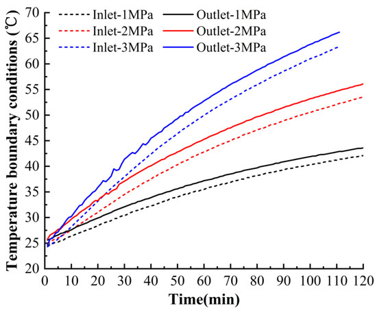
Figure 13.
Inlet and outlet temperatures of the valve orifice obtained via measurement.
4.3. Analysis of Simulation Results
On the basis of the fluid–solid–heat coupling simulation, the temperature fields at different inlet pressures, valve opening of 1 mm and moment of 60 min are presented in Figure 14 to analyze the relationship amongst pressure drop, fluid velocity and temperature in the valve orifice. As indicated in Figure 14a–c, a wake flow was generated at the rear end of the valve orifice, and the fluid velocity near the sharp edge was higher than that in other locations in the flow field. When the inlet pressures were 1 MPa, 2 MPa and 3 MPa, the maximum fluid velocities of the wake flows were 45 m/s, 65 m/s and 80 m/s, respectively, and the highest temperatures in the valve orifices were 42 °C, 56 °C and 65 °C, respectively (indicated in Figure 14a–c). This result means that the large pressure drop led to high fluid velocity and increased the temperature of the valve orifice.
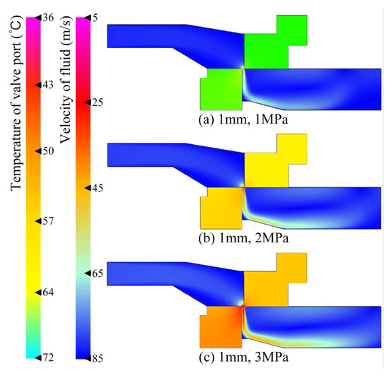
Figure 14.
Temperature field of the valve orifice and fluid velocity at different inlet pressures, valve opening of 1 mm with time at 60 min.
The thermal deformation of the valve orifice corresponding to Figure 14 after calculation with the static–structural module is indicated in Figure 15. When the inlet pressures were 1 MPa, 2 MPa and 3 MPa, the corresponding thermal deformations were 4.1 μm, 6.9 μm and 9.4 μm, respectively, which means that under the same valve opening, thermal deformation increased while pressure dropped.
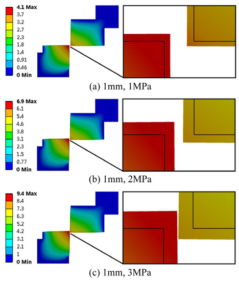
Figure 15.
Thermal deformation at different inlet pressures, valve opening of 1 mm and with time at 60 min (magnified 30 times).
4.4. Accuracy Verification of Simulation
The temperature results of the measurement and simulation and the deformation results of M-OA and the simulation at 60 min are presented in Table 3.
Table 3.
Temperature and deformation results at 60 min.
The simulation results were close to the measurement and M-OA results, but the accuracy of the simulation needs to be verified using a larger amount of data than that used in this study. Thus, it was necessary to compare all the results obtained within the timeframe of the entire experiment with the results of the simulation. M(t) represented the time-varying result obtained by measurement or the M-OA method, and S(t) denoted the time-varying result obtained by simulation. If M(t) is taken as the criterion, the accuracy of S(t) can be expressed as Equation (9) and used to calculate the accuracy of the temperature and deformation simulation results. At inlet pressures of 1 MPa, 2 MPa and 3 MPa, the upper limit of the integral function t equaled the experiment time at 120 min, 120 min and 110 min, respectively.
By averaging the accuracy results at 1 MPa, 2 MPa and 3 MPa, the accuracy of the simulation can be obtained as
The accuracy of the temperature and deformation simulation results was calculated and is presented in Table 4.
Table 4.
Accuracy of the simulation.
The accuracy rate of the temperature simulation result was 95%, indicating that the unidirectional fluid–solid–heat coupling method in Fluent can calculate the temperature of the hydraulic valve orifice with precision. The accuracy rate of the deformation simulation result was 82.7%, which is lower than that of the temperature simulation result; nevertheless, it can still reveal the thermal deformation field or provide a rough estimate for users.
5. Discussion
The measurement, M-OA and simulation results were compared and analyzed at a valve opening of 1 mm, inlet pressure of 3 MPa and time range of 1 min to 110 min, as presented in Figure 16. The temperature of the sharp edge was selected as a characteristic parameter because the temperature in the valve orifice was distributed unevenly.
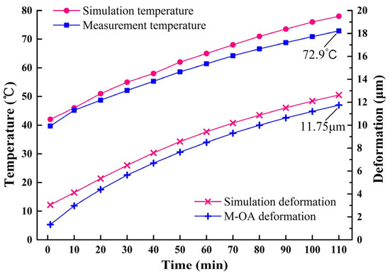
Figure 16.
Relationship between the temperature and deformation of the valve orifice when valve opening is 1 mm and inlet pressure is 3 MPa.
As indicated in Figure 16, the temperature of the sharp edge increased with time, and the thermal deformation of the valve orifice increased synchronously. The simulated temperature results were higher than the measurement results, and the simulated deformation results were higher than the M-OA results. In the measurement and M-OA results, at 110 min, the temperature of the sharp edge reached 72.9 °C, and the thermal deformation reached 11.75 μm. The edge length of the planar valve core is 18 mm, equal to a radius of the cylindrical spool valve of Φ36 mm, so the thermal deformation of the planar valve core is close to unilateral thermal deformation of a cylindrical spool.
On the basis of the quantitative results calculated by M-OA method, a spool valve of Φ36 mm will be taken as the research object to evaluate the risk of spool clamping. Table 5 shows the machining accuracy of a frequently used Φ36 mm spool valve, including the diameter and roughness of the spool and valve hole. The roughness is small enough to be ignored when the unilateral clearance range of the spool valve is determined, so the unilateral clearance range is calculated by the upper and lower deviation of the spool and valve hole. The minimum and maximum sizes of unilateral clearance are 5 μm and 7.5 μm, respectively; the two values will be taken as the evaluation criteria of spool clamping.
Table 5.
Unilateral clearance range of a Φ36 spool valve.
The orthogonal decomposition of the M-OA deformation curve (as Figure 16 shows) can be marked as ‘ld’ and equals of thermal deformation of the sharp edge. The minimum and maximum size of unilateral clearance is marked as ‘lc(min)’ and ‘lc(max)’, respectively. The micro-mechanism of spool clamping caused by thermal deformation can be seen in Figure 1. As Figure 17 indicates, when the temperature of the sharp edge of the valve orifice is taken as the abscissa, ‘ld’ increases with the temperature. Before 56.7 °C, ld < lc(min), and there is no risk of clamping; between 56.7 °C and 68.7 °C, lc(min) < ld < lc(max), and the risk of clamping rises continuously; after 68.7 °C, lc(max) < ld, and the spool clamping will generate inevitably. At 72.9 °C, ld is approximately 8.3 μm.
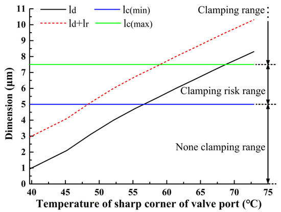
Figure 17.
Evaluation of spool clamping caused by thermal deformation.
It is noteworthy that the spool clamping is not only caused by thermal deformation of the spool but also by thermal deformation of the valve hole; what is more, the spool can also generate a radial displacement when sliding in the valve hole. The extra deformation and displacement are combined and marked as ‘lr’. lr is determined by the processing technology and assembly process, so it is not a certain value. As Figure 17 shows, compared with the curve of ld, the curve of ld + lr in the clamping risk range and clamping range increased obviously, which means that the clamping risk will rise when thermal deformation of the valve hole and radial displacement of the spool are taken into consideration.
6. Conclusions
The main conclusions are as follows:
- The proposed optimization algorithm based on measurement data (M-OA) can be successfully implemented in calculating the thermal deformation of a hydraulic valve orifice with an uneven temperature distribution. When the sharp edge was at a temperature of 60 °C, the thermal deformation results obtained via observation and M-OA were 7.7 μm and 7.62803 μm, respectively, indicating that the M-OA method is reliable in calculating thermal deformation.
- A large drop in pressure leads to a rapid increase in temperature and causes serious deformation. When the inlet pressures were 1 MPa, 2 MPa and 3 MPa, the temperatures in the sharp edge of the valve orifice reached 41.9 °C, 52.8 °C and 61.4 °C, respectively, and thermal deformation within 60 min was measured at 3.85 μm, 6.71 μm and 8.5 μm, respectively.
- The accuracy rates of the temperature and deformation results calculated via Fluent and Workbench joint simulation are acceptable. When the measurement and M-OA results served as criteria, the accuracy rate of the temperature result calculated with the fluid–solid–heat method reached 95%, and that of the deformation result obtained with the static–structural module reached 82.7% when the inlet pressure ranged from 1 MPa to 3 MPa.
- Spool clamping is considerably affected by the relationships between unilateral clearance lc, radial fretting allowance lr and radial thermal deformation ld. In this study, ld reached 8.3 μm when the temperature of the sharp edge rose to 72.9 °C, meaning that the value of ld is high enough to cause spool clamping for a spool valve of Φ36 mm, with unilateral clearance lc ranging from 5 μm to 7.5 μm. When the radial fretting allowance lr, including thermal deformation of spool and extra displacement, is taken into consideration, there is a higher risk of clamping.
The purpose of this study is to offer a method for measuring the temperature of valve orifices and an optimization algorithm for thermal deformation, as well as to verify the accuracy of Fluent and Workbench joint simulation using the measurement and M-OA results. For such reasons, the simplified valve orifice is only used as a carrier of the technology and method, and the thermal deformation of the valve hole and radial displacement of the spool have not undergone quantitative research. Therefore, the micro-mechanism of spool clamping is still in the stage of theoretical analysis. In future work, other factors besides thermal deformation of the valve orifice will be taken into consideration for an in-depth study.
Author Contributions
Conceptualization, supervision, project administration, funding acquisition, H.J.; methodology, data curation, writing—original draft preparation, Q.C.; software, validation, visualization, H.Z.; investigation, formal analysis, writing—review and editing, J.Z. All authors have read and agreed to the published version of the manuscript.
Funding
This research was funded by the National Natural Science Foundation of China, grant number 51575254.
Acknowledgments
This study was funded in part by Lanzhou University of Technology National and Provincial Excellent Doctoral Dissertation Cultivation Methods.
Conflicts of Interest
The authors declare no conflict of interest.
References
- Lisowski, E.; Filo, G.; Rajda, J. Pressure compensation using flow forces in a multi-section proportional directional control valve. Energy Convers. Manag. 2015, 103, 1052–1064. [Google Scholar] [CrossRef]
- Lisowski, E.; Czyzycki, W.; Rajda, J. Three dimensional CFD analysis and experimental test of flow force acting on the spool of solenoid operated directional control valve. Energy Convers. Manag. 2013, 70, 220–229. [Google Scholar] [CrossRef]
- Aung, N.Z.; Peng, J.; Li, S. Reducing the Steady Flow Force Acting on the Spool by Using a Simple Jet-Guiding Groove. In Proceedings of the 2015 International Conference on Fluid Power and Mechatronics (FPM), Harbin, China, 5–7 August 2015. [Google Scholar]
- Lee, G.S.; Sung, H.J.; Kim, H.C.; Lee, H.W. Flow Force Analysis of a Variable Force Solenoid Valve for Automatic Transmissions. J. Fluids Eng. 2010, 132, 031103. [Google Scholar] [CrossRef]
- Chen, Q.; Ji, H.; Zhu, Y.; Yang, X. Proposal for Optimization of Spool Valve Flow Force Based on the MATLAB-AMESim-FLUENT Joint Simulation Method. IEEE Access 2018, 6, 33148–33158. [Google Scholar]
- Borghi, M. Hydraulic locking-in spool-type valves: Tapered clearances analysis. Proc. Inst. Mech. Eng. Part I J. Syst. Control Eng. 2001, 215, 157–168. [Google Scholar] [CrossRef]
- Wei, M.; Yang, S.; Wu, L.; Liu, S. Simulation and Experiment on the Flow Field in Fit Clearance for a Large Size Spool Valve. In Proceedings of the 2011 International Conference on Fluid Power and Mechatronics, Beijing, China, 17–20 August 2011. [Google Scholar]
- Park, T.J.; Hwang, Y.G. Effect of Groove Sectional Shape on the Lubrication Characteristics of Hydraulic Spool Valve. Tribol. Online 2010, 5, 239–244. [Google Scholar] [CrossRef][Green Version]
- He, T.; Wang, C.; Huang, S.; Tian, D. Effect of micro-topography on the lubrication and leakage characteristics of a micro-texture valve core. J. Beijing Univ. Chem. Technol. 2016, 43, 110–116. [Google Scholar]
- Han, L.; Wang, S.; Zhang, C. A partial lubrication model between valve plate and cylinder block in axial piston pumps. Proc. Inst. Mech. Eng. Part C J. Mech. Eng. Sci. 2015, 229, 3201–3217. [Google Scholar] [CrossRef]
- Fan, M.; Zeng, Z.; Kang, R.; Zio, E. Reliability Modeling of a Spool Valve Considering Dependencies Among Failure Mechanisms. In Proceedings of the 25th European Safety and Reliability Conference, ESREL, Zurich, Switzerland, 7–10 September 2015. [Google Scholar]
- Fan, S.; Xu, R.; Ji, H.; Yang, S.; Yuan, Q. Experimental Investigation on Contaminated Friction of Hydraulic Spool Valve. Appl. Sci. 2019, 9, 5230. [Google Scholar] [CrossRef]
- Ji, H.; Cui, T.X.; Chen, X.M.; Min, W.; Zheng, Z.; Liu, X.Q. Rotation phenomenon of square micron particles in clearance of spool valve. J. Lanzhou Univ. Technol. 2017, 43, 51–55. (In Chinese) [Google Scholar]
- Zhou, Z.; Jin, G.; Tian, B.; Ren, J. Hydrodynamic force and torque models for a particle moving near a wall at finite particle Reynolds numbers. Int. J. Multiph. Flow 2017, 92, 1–19. [Google Scholar] [CrossRef]
- Tanaka, Y.; Oba, G.; Hagiwara, Y. Experimental study on the interaction between large scale vortices and particles in liquid–solid two-phase flow. Int. J. Multiph. Flow 2003, 29, 361–373. [Google Scholar] [CrossRef]
- Liu, X.; Ji, H.; Min, W.; Zheng, Z.; Wang, J. Erosion behavior and influence of solid particles in hydraulic spool valve without notches. Eng. Fail. Anal. 2020, 108, 104262. [Google Scholar] [CrossRef]
- Yuan, H.; Ji, H.; Zhang, J.; Liu, X.; Chen, Q.; Zheng, Z.; Peng, G. Visualization Experiment of Single Particle Motion in Model of Spool Valve Clearance. In Proceedings of the 2019 IEEE 8th International Conference on Fluid Power and Mechatronics (FPM), Wuhan, China, 10–13 April 2019. [Google Scholar]
- Deng, J.; Shao, X.M.; Fu, X.; Zheng, Y. Evaluation of the viscous heating induced jam fault of valve spool by fluid–structure coupled simulations. Energy Convers. Manag. 2009, 50, 947–954. [Google Scholar] [CrossRef]
- Yuan, W.B.; Ji, H.; Yang, X.B.; Li, D.M. Influence of the Throttle Groove Number on the Valve Spool Thermal Deformation. Hydraul. Pneum. Seals 2019, 39, 17–20. [Google Scholar]
- Ji, H.; Yong, C.; Wang, Z.; Yang, W. Numerical Analysis of Temperature Rise by Throttling and Deformation in Spool Valve. In Proceedings of the 2011 International Conference on Fluid Power and Mechatronics, Beijing, China, 17–20 August 2011. [Google Scholar]
- Angadi, S.V.; Jackson, R.L.; Choe, S.Y.; Flowers, G.T.; Suhling, J.C.; Chang, Y.-K.; Ham, J.-K. Reliability and life study of hydraulic solenoid valve. Part 1: A multi-physics finite element model. Eng. Fail. Anal. 2009, 16, 874–887. [Google Scholar] [CrossRef]
- Angadi, S.V.; Jackson, R.L.; Choe, S.Y.; Flowers, G.T.; Suhling, J.C.; Chang, Y.-K.; Ham, J.-K.; Bae, J.-I. Reliability and Life Study of Hydraulic Solenoid Valve. Part 2: Experimental Study. Eng. Fail. Anal. 2009, 16, 944–963. [Google Scholar] [CrossRef]
- Zhao, J.; Zhou, S.; Lu, X.; Gao, D. Numerical simulation and experimental study of heat-fluid-solid coupling of double flapper-nozzle servo valve. Chin. J. Mech. Eng. 2015, 28, 1030–1038. [Google Scholar] [CrossRef]
- He, J. Valve Body Thermal Stress Control While Warming Up. In Proceedings of the ASME Turbo Expo 2017: Turbomachinery Technical Conference and Exposition, Charlotte, CA, USA, 26–30 June 2017. [Google Scholar]
- Maher, A.R.; Al-Baghdadi, S. Mechanical and thermal stresses analysis in diesel engine exhaust valve with and without thermal coating layer on valve face. Int. J. Energy Environ. 2016, 7, 253–262. [Google Scholar]
- Wu, B.; Li, J.; Li, J.; Shao, J. Research on the Thermal Deformation Field of Exhaust Valve for High Temperature Steam Booster Pump Based on ANSYS. In Proceedings of the 2011 International Conference on Electronic & Mechanical Engineering and Information Technology, Harbin, China, 12–14 August 2011. [Google Scholar]
- Zhou, J.L.; Shi, M.; Zhang, P.Y.; Yang, G.Y.; Yu, R.; Dai, Y. Research on Hot Deformation Behavior of 45 Steel in Low Temperature Region. Iron Steel 2014, 49, 62–65, 75. (In Chinese) [Google Scholar]
- Ren, Q.; Wang, L.; Huang, Q. A Micro-Test Structure for the Thermal Expansion Coefficient of Metal Materials. Micromachines 2017, 8, 70. [Google Scholar] [CrossRef]
- Soares, A.R.; Pontón, P.I.; Mancic, L.; D’Almeida, J.R.M.; Romao, C.P.; White, M.A.; Marinkovic, B.A. Al2Mo3O12/polyethylene composites with reduced coefficient of thermal expansion. J. Mater. Sci. 2014, 49, 7870–7882. [Google Scholar] [CrossRef]
- Hu, X.; Hemmat, Z.; Majidi, L.; Cavin, J.; Mishra, R.; Salehi-Khojin, A.; Ogut, S.; Klie, R.F. Controlling Nanoscale Thermal Expansion of Monolayer Transition Metal Dichalcogenides by Alloy Engineering. Small 2020, 16, 1905892. [Google Scholar] [CrossRef] [PubMed]
- Vetterli, M.; Tavangar, R.; Weber, L.; Kelly, A. Influence of the elastic properties of the phases on the coefficient of thermal expansion of a metal matrix composite. Scr. Mater. 2011, 64, 153–156. [Google Scholar] [CrossRef]
- Xuan, H.; Amirhossein, B.; Serdar, O.; Salehi, A.; Klie, R.F. Tailoring Thermal Expansion Coefficient of Transition Metal Dichalcogenides via Alloy Engineering. Microsc. Microanal. 2018, 24, 1560–1561. [Google Scholar]
- Aggarwal, R.L.; Fan, T.Y. Thermal diffusivity, specific heat, thermal conductivity, coefficient of thermal expansion, and refractive-index change with temperature in AgGaSe2. Appl. Opt. 2005, 44, 2673–2677. [Google Scholar] [CrossRef]
- Yang, S.; Zhang, J.Y.; Yang, Y.-Y.; Huang, J.-Y.; Bai, Y.-R.; Zhang, Y.; Lin, X.-C. Automatic compensation of thermal drift of laser beam through thermal balancing based on different linear expansions of metals. Results Phys. 2019, 13, 102201. [Google Scholar] [CrossRef]
- Wang, Z.; Yuan, Y. Micromechanics-based modeling of elastic modulus and coefficient of thermal expansion for CNT-metal nanocomposites: Effects of waviness, lustering and aluminum carbide layer. Int. J. Mech. Mater. Des. 2020, 8, 1–17. [Google Scholar] [CrossRef]
- Wang, Q.K. Studies on the Linear Expansion Coefficientof Metal. J. Anhui Norm. Univ. 2018, 41, 440–443. [Google Scholar]
© 2020 by the authors. Licensee MDPI, Basel, Switzerland. This article is an open access article distributed under the terms and conditions of the Creative Commons Attribution (CC BY) license (http://creativecommons.org/licenses/by/4.0/).