Evaluation of Water Hammer for Seawater Treatment System in Offshore Floating Production Unit

Abstract

Water hammer can result in the rupture of pipes, and significant damage to pipe supports is inevitable during the operation of an offshore plant. In this study, the dynamic behaviors of the water hammer caused by closing valves and starting pumps for the seawater treatment system were evaluated by using the 1D numerical simulation model based on the method of characteristics. Before conducting an analysis of a complex piping network, the 1D numerical simulation tools were validated by a comparison between the numerical results and the results from both static and transient experiments that have been conducted in other studies. For the case study, the effects of valve flow characteristics and valve closing time on surge pressure were investigated, and the equal percentage butterfly valve was recommended in order to reduce the surge pressure with a shorter valve closure time and lower weight compared to other valve types.

1. Introduction

The seawater distribution system in an offshore structure is designed to provide seawater at appropriate pressures for the water injection system, heat exchanger, and utility water service. For economic reasons, engineers determine the optimized pipe size considering design loading conditions with a safety margin in order to minimize the required overall cost. However, such a conventional design could overlook the dynamic variables in the event of a hydraulic transient since the design loading condition was static loading. There are inevitable transient events, referred to as water hammer phenomenon, that are caused by the opening/closing of valves and the start-up/shutdown of pumps in seawater distribution systems. When there is a sudden change of the flow, a pressure wave propagates at sonic velocity through the pipe against the flow [1]. As a result, the fluid between the pressure wave front and the valve is compressed, and a sudden increase in the pressure on the piping system can occur.

Many experimental and numerical studies have been conducted to understand the water hammer phenomenon. Simpson [2] conducted a series of experiments to investigate a short duration pressure pulse due to a cavity collapse. The experiments were performed in a sloped piping system with a reservoir, and the results were simulated later using a discrete vapor-cavity model (DVCM) [3]. Kwon [4] investigated the transient flow in a piping system using both experimental and numerical models, and it was shown that the numerical method could simulate the transient flow due to the water hammer well using the 1D method of characteristics (MOC).

In recent studies, the 3D computational fluid dynamic (CFD) simulation was widely used to evaluate the water hammer phenomenon. Jinping et al. [5] simulated the water hammer using the Navier–Stokes equation, and showed the possibility of the CFD method for the water hammer which has unsteady and highly nonlinear characteristics. Martin [6] tried to correlate 3D CFD and the 1D MOC with the evaluation of the water hammer phenomenon. The results from the 3D CFD are in good agreement with the result of the 1D MOC analysis considering the unsteady friction. This implies that the 3D pipe model is able to capture damping resulting from unsteady wall friction.

However, previous researchers have limited the CFD models to simple, short pipelines due to time-consuming computational work and difficulties in implementing the fluctuations in the wake of the wave front [7]. In order to overcome the limitations of the 3D CFD model, the 1D–3D coupling method was introduced [8]. In this coupling method, the compressible water hammer can be simulated by utilizing the advantages of the 1D and 3D approaches. The study also showed the necessity of improving the coupling method for a complex geometry piping network system with lots of fittings.

The existing papers that deal with water hammer have been limited to a single pipe, and the investigation of an offshore piping system installed in a limited area is rare. In this study, the water hammer that occurred in an offshore floating production unit was investigated with various operating scenarios using 1D numerical simulation based on MOC which is shown as a proper method to be applied for the piping system. The effects of the primary factors, such as the characteristics of the valve and the valve’s closure time were analyzed, and recommendations were suggested with the goal of preventing or reducing the damage caused by water hammer.

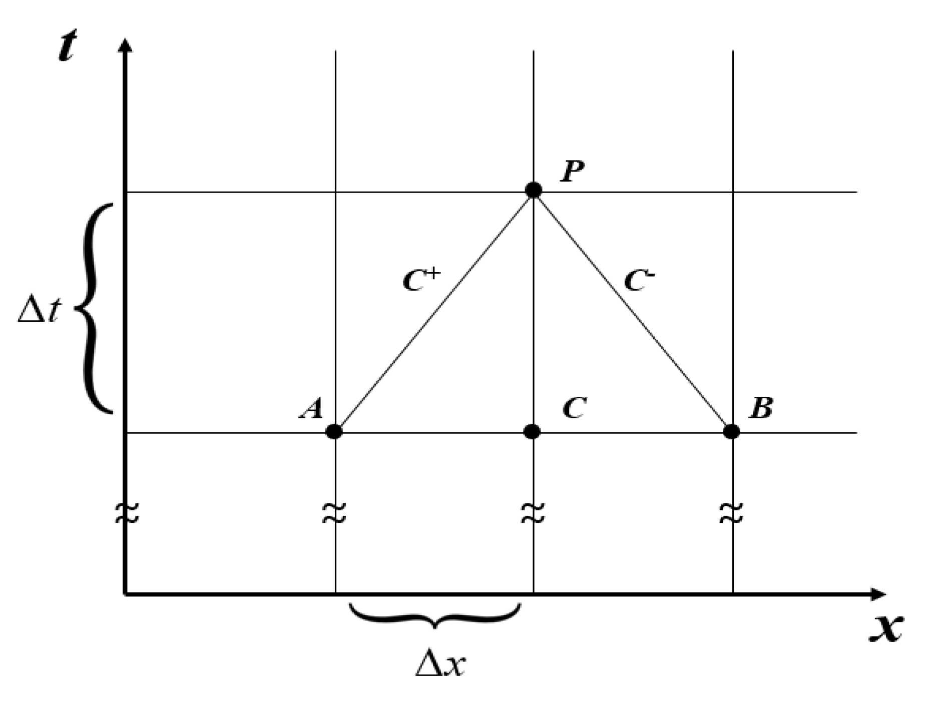
2. Mathematical Model

The fundamental equations for 1D unsteady-state flow in a pipe were derived from mass conservation and energy conservation laws. The classical mass and momentum equations for 1D water hammer have been refined by several studies since a general theory of water hammer was developed as Equations (1) and (2) [9]:

$$\frac{a^2}{g}\frac{\partial V}{\partial x}+\frac{\partial H}{\partial t}=0$$

(1)

$$\frac{\partial V}{\partial t}+g\frac{\partial H}{\partial x}+\frac{4}{\rho D}{\tau }_w=0$$

(2)

where $a$ is the acoustic pressure wave speed,$g$ is the gravitational acceleration, $\rho$ is the density of the fluid, $V$ is the cross-section average velocity, $H$ is the piezo-metric head which means the sum of the elevation head with the pressure head, D is the diameter of the pipe, ${\tau }_w$ is the wall shear stress, and x is the spatial coordinate along the pipe.

Equations (1) and (2) are characterized as the continuity equation and the momentum equation, respectively, for the 1D water hammer phenomenon, and they include the physics required to model the propagation of a wave in a complex piping network. The following assumptions were made:

• Homogeneous fluid;
• Linearly elastic fluid and pipe wall;
• One-dimensional flow;
• Longitudinal stresses (Poisson’s effect) are neglected;
• Inertia of the pipe is neglected.

Equation (3) was introduced to relate the wave speed to the properties of the fluid and the pipe where the typical wave speed during the water hammer ranged from 700 to 1400 m/s [10]:

$$\frac{1}{a^2}=\frac{\rho }{K_f}+\frac{\rho }{E \left(\epsilon /D\right)}$$

(3)

where $K_f$ is the fluid elastic bulk modulus, $\epsilon$ is the thickness of the wall of the pipe, and E is the elastic modulus.

With respect to Equation (2), it is essential to consider the wall shear term carefully to avoid underestimating the energy decay after the first wave cycle. The conventional model, i.e., the so-called quasi-steady wall shear model, assumed that the friction expression at the pipe wall remains valid during a transient event. However, one study found that, after the first wave cycle, there are discrepancies between the numerical results of the conventional model and the experimental results [11]. In order to correct the discrepancies in the friction expression, several studies have suggested empirical-based corrections to the quasi-steady wall shear model (Equation (4)):

$${\tau }_w={\tau }_{ws}+{\tau }_{wu}$$

(4)

where ${\tau }_{ws}$ is the quasi-steady wall shear stress, and ${\tau }_{wu}$ is the discrepancy between the unsteady and quasi-steady stress. After performing laboratory experiments, Dailly et al. [12] noted that ${\tau }_{wu}$ should be negative for decelerating flows and positive for accelerating flows. Shuy [13] discussed the decreases in wall shear stress and concluded that it was due to flow re-laminarization. Brunone et al. [14] proposed an important modification of the unsteady friction model, which has been used most commonly for the analysis of water hammer as Equation (5). A proposed empirical method to estimate the k parameter was based on fitting the experimentally measured history of the decay of pressure head:

$${\tau }_{wu}=\frac{k\rho D}{4}\left(\frac{\partial V}{\partial t}-a\frac{\partial V}{\partial x}\right)$$

(5)

It has been shown that the numerical results from this model were in good agreement with the experimental result. The method of characteristics solves governing Equations (1) and (2) by converting two partial differential equations into a pair of formulas to calculate the pressure head and velocity with spatial and temporal discretization (Equation (6)) [15]. The fixed-grid MOC allows the easy calculation of both the velocity fields and pressure in space at a given time. The fixed-grid MOC was used successfully to evaluate the water hammer phenomenon in piping networks and systems. The x–t grid was selected to ensure the characteristic C⁺ and C⁻ curves as defined by Equation (7) [16] and shown in Figure 1:

$$\frac{dV}{dt}\pm \frac{g}{a}\frac{dH}{dt}+\frac{{\tau }_w\pi D}{\rho }=0$$

(6)

$$\frac{∆x}{∆t}=\pm a$$

(7)

Many 1D simulation software programs for water hammer have been developed in recent years. Compared to other programs, PIPENET (Sunrise Systems Limited, Cambridge, UK) [17] is more suitable for the case study because it offers automatic wave-speed calculation, cavitation options and valve-opening profiles for each section.

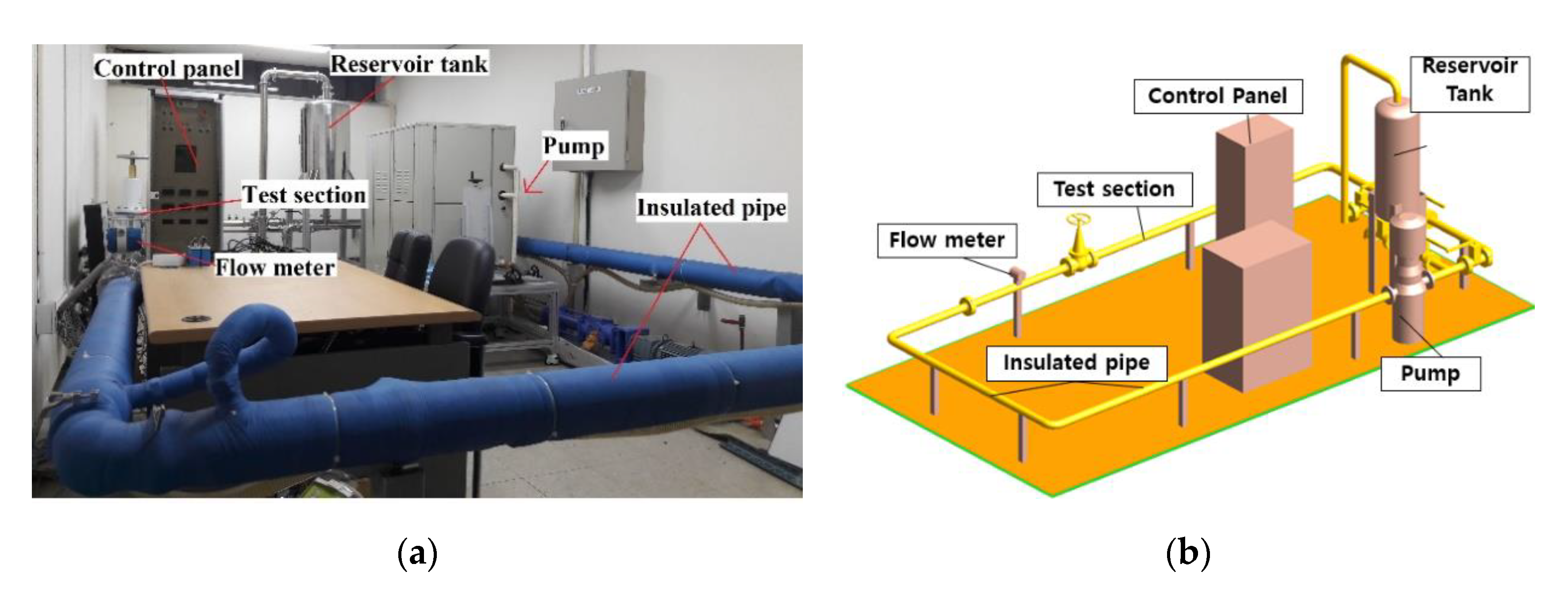
3. Validation of the 1D Simulation Model

In this study, the validation was performed to verify the reliability of the case study that was conducted in this study using PIPENET. The 1D numerical simulation model was validated by comparing the numerical results with the results from both static and transient experiments performed in other studies [18,19]. After verification, a case study with respect to the seawater treatment system was performed.

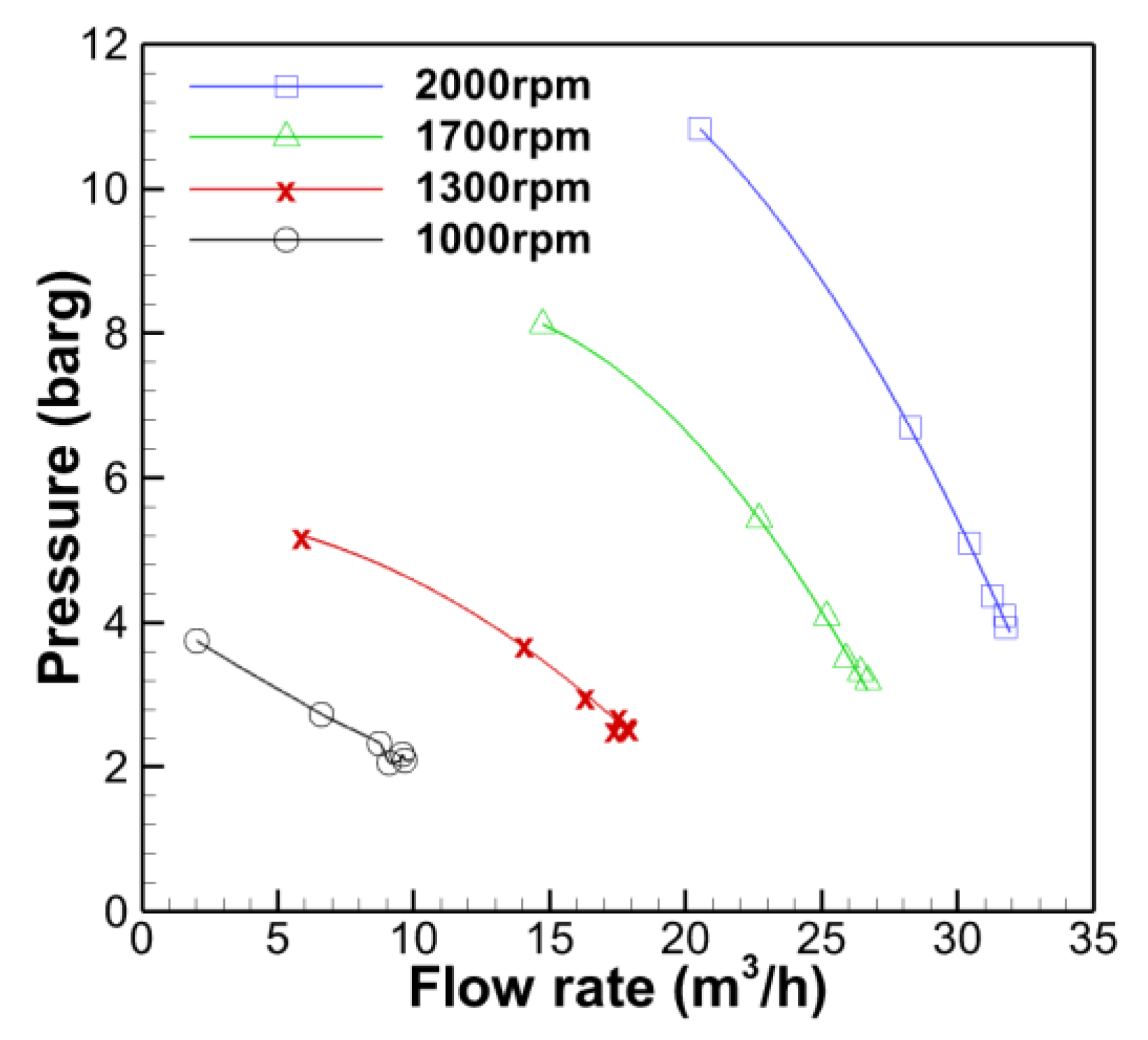
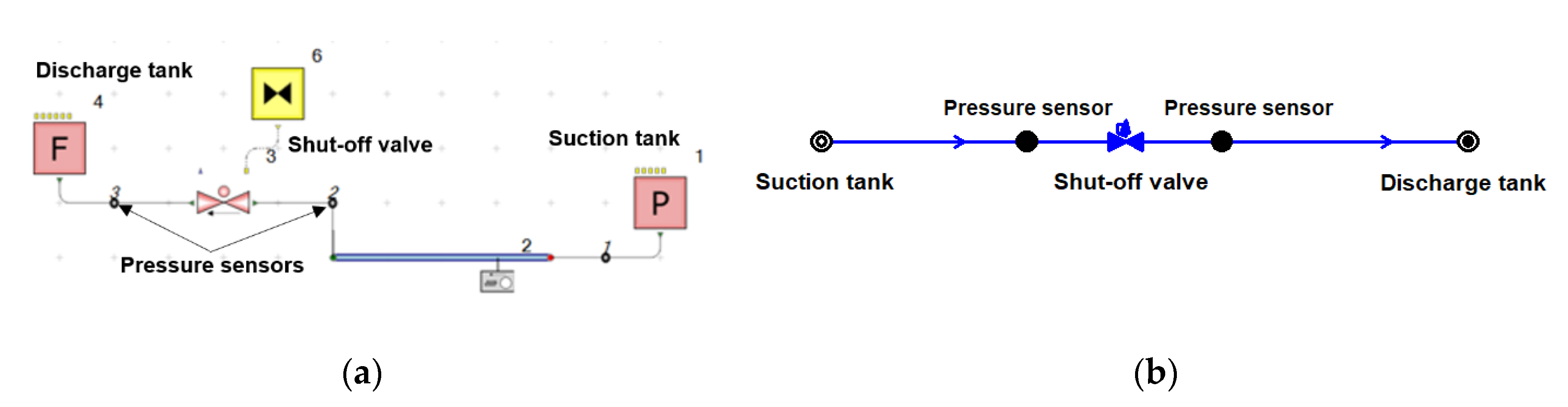
3.1. Validation for the 1D Steady State Simulation Model

A series of experiments was carried out in a flow loop at Pusan National University. The loop was comprised of a pump, reservoir tank, flowmeter, globe valve, an 18 m pipe that had a 3 inch diameter, and other fittings. Figure 2a shows the flow loop facilities and Figure 2b shows the 3D model with the main components. In this test, Nguyen et al. [18] investigated the inherent characteristic and the installed characteristic of the valve, the valve openings could range from 10% to 100%, and the range of the pump was varied between 1000 and 2000 rpm. The flow rate and the pressure distributions along the pipe from the upstream to the downstream of the globe valve were measured using a flow meter and pressure sensors, respectively.

The performance of the pump was measured for each rpm setting (Figure 3), and the calculated flow coefficient (Figure 4) based on the flowrate and the pressure were inputs, and they could be selected depending on the different opening ratios. The Colebrook–White pressure drop model [20] was chosen, and the inlet/outlet pressure boundary condition was set to be at the pump’s suction and at +10D from the downstream of the valve, respectively. Water at the temperature of 20 °C was used as the simulation fluid.

Figure 5 shows the established flow-loop in PIPENET v1.6.

Figure 6 shows the effect of the flow coefficient on pressure drop for various pump speed (Figure 6a–d). In case of a valve opening of 20%, which has the corresponding velocity below 1.4 m/s and a Reynolds numbers below 10⁵, there was a remarkable difference when using the inherent flow coefficient. However, when the valve opening was 30% or more, the simulation results were generally in good agreement with the experimental results, i.e., the errors were less than 10%. In addition, it was found that, when using the installed valve flow characteristics, the agreement with the experimental values was better than when the inherent valve flow characteristics were used.

The differences of pressure drop for the two different flow coefficients (Figure 6) are summarized in Figure 7. It could be seen that the results of pressure drop from the simulation agreed well with the experimental results, especially at a relatively high Reynolds number (Re), when the pump speed was high. The differences using the inherent flow coefficient (Figure 7a) showed higher differences of about 60% at maximum when the Re was relatively lower, meanwhile those with the installed flow coefficient (Figure 7b) showed much smaller differences. It is because the characteristics of the valve in the piping system were not included in the coefficient [18]. In this study, the inherent flow coefficient at high Re was used for the simulation of the seawater treatment system.

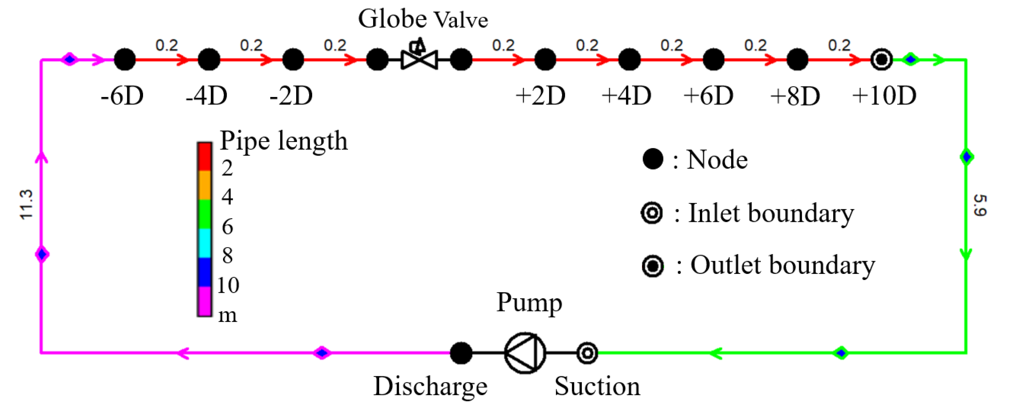
3.2. Validation for 1D Transient Analysis

Laboratory tests were performed to investigate the water hammer events in pipelines. The laboratory facility consists of a copper pipe that was 37.23 m long and was connected to two pressurized tanks [19]. A computerized system controlled the pre-determined pressure in each of the tanks. Rapid closure of the valve was done by either a valve actuator or manually. Five pressure sensors were installed along the pipeline. The static pressure head in an upstream end tank was 32 m, and the tests were conducted at each flow velocity in the range from 0.1 to 0.3 m/s. Based on the data from the experiment in

Table 1. Parameters of the piping system for the analysis of water hammer.

Properties	Value
Outside diameter (OD)	22.1 mm
Wall thickness of the pipe (e)	1.63 mm
Roughness	0.0013 mm
Wave speed	1319 m/s
Water density at 15.4 °C	999 kg/m3
Vapor pressure	0.02062 barg
Total simulation time	1 s
Total length of the pipe	37.23 m

, piping with one shut-off valve was installed in FLOWMASTER v7 (Mentor Graphics, Wilsonville, OR, USA) [21] and PIPENET v1.6. The same boundary condition as the test was determined at the upstream and downstream ends, as shown in Figure 7. It was assumed that the experimentally determined wave speed of 1319 m/s was applied to the simulation model. The time step ∆t = 0.0017641 s and the grid size of ∆x = 2.3268 m were determined to meet the Courant stability criterion as Equation (8) [22]:

$$\frac{∆t}{∆x}\le \frac{1}{a}$$

(8)

The time required to fully close the shut-off valve was 0.009 s. Figure 8 show the schematic diagrams of the simulation setup in FLOWMASTER (Figure 8a) and in PIPENET (Figure 8b).

Figure 9 shows the pressure change over time according to different flow velocities that ranged from 0.1 to 0.3 m/s (Figure 9a–c). It was found that the simulation results from both PIPENET and FLOWMASTER agreed well with the experimental results until the second pressure wave period. The peak pressure occurred at approximately 9 Hz. Since the PIPENET software was based on the quasi-steady friction model, long-term decay tends to be underestimated, but the FLOWMASTER provided an unsteady friction model and showed good agreement with the experimental results. However, PIPENET offered wave-speed automatic calculation, cavitation options, and valve-opening profiles for each section, making it a more suitable type for future studies on the seawater treatment system, which has more complex piping systems.

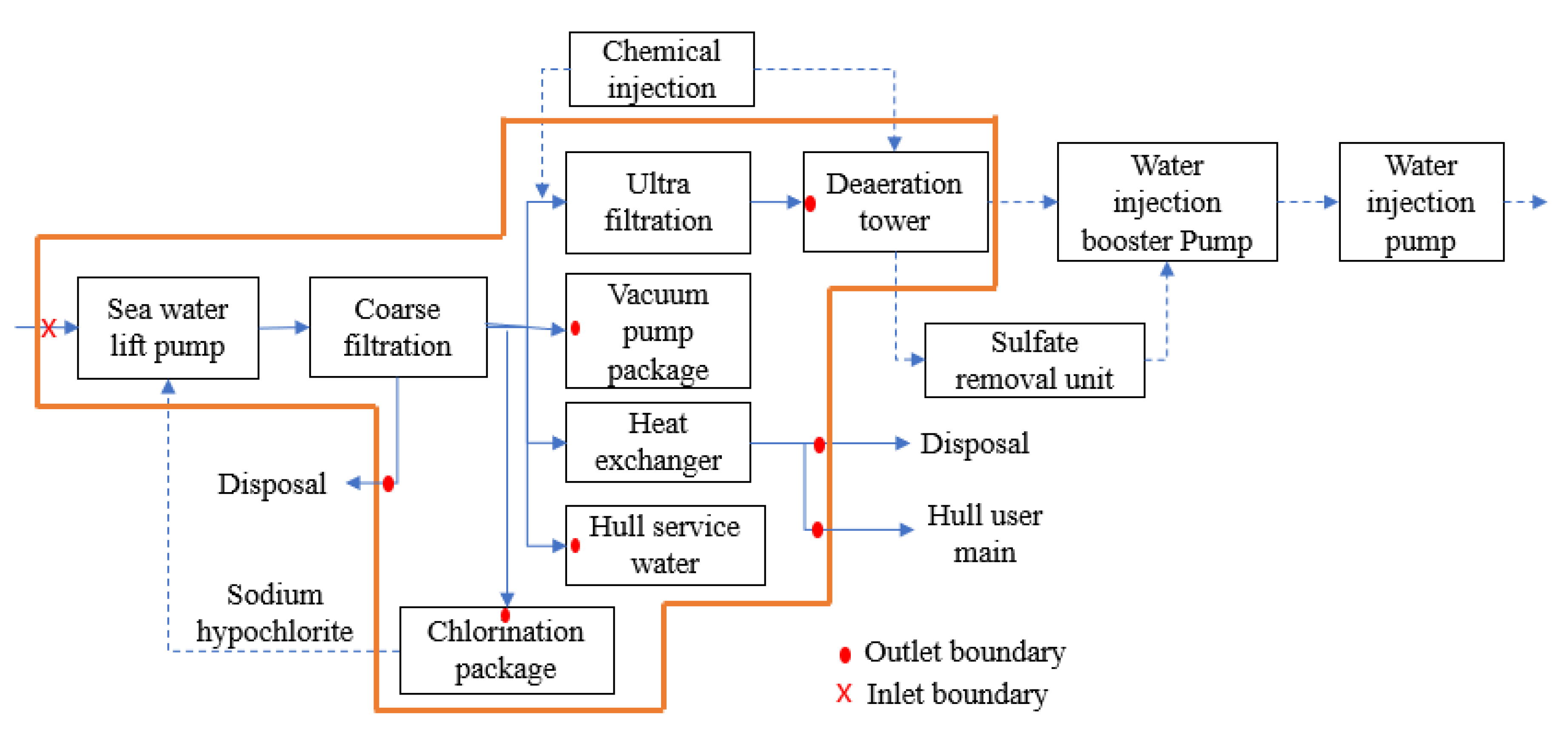
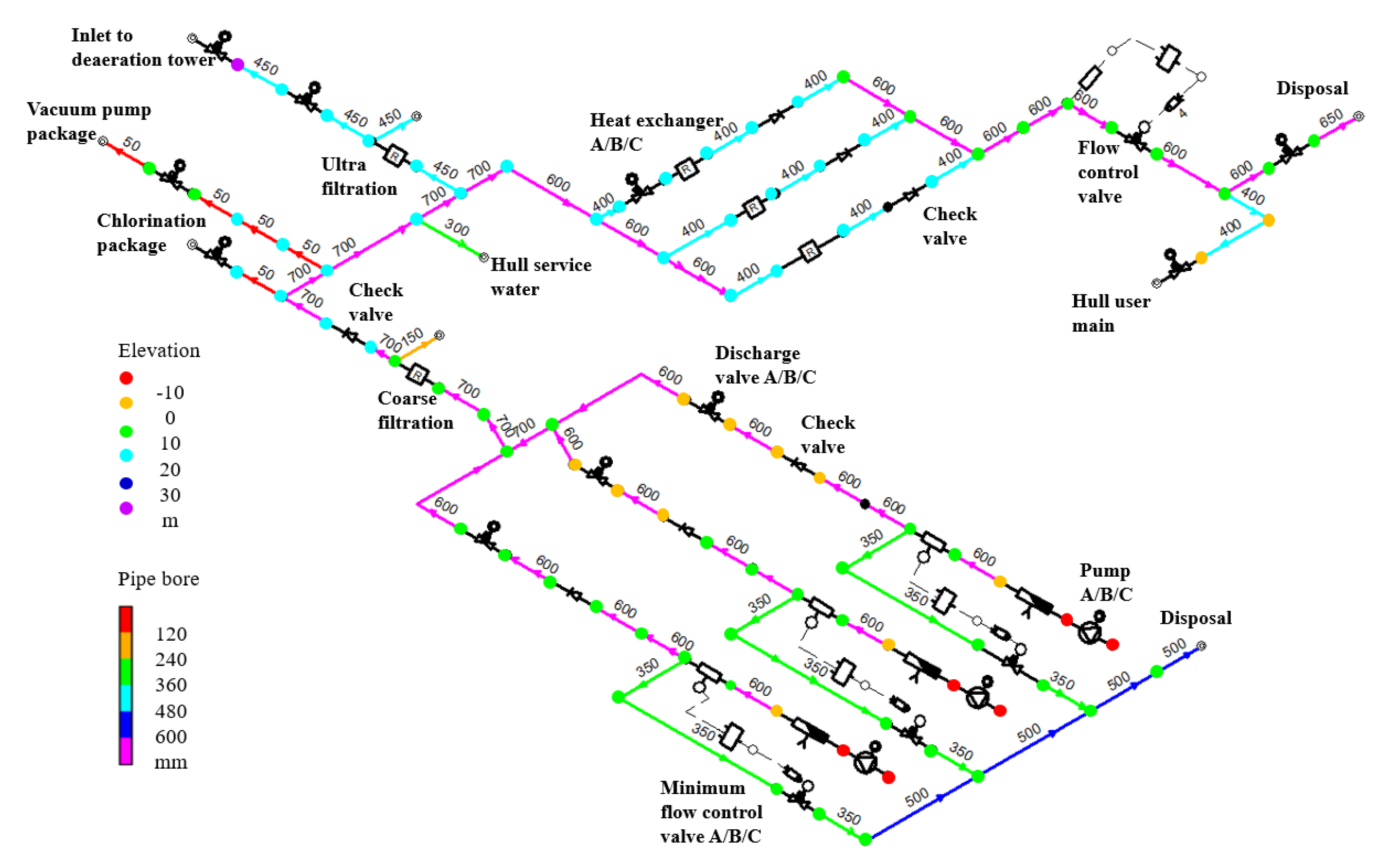
4. Case Study: Seawater Treatment System

To perform the analysis on an actual piping network, we chose a seawater treatment system in a floating production unit (FPU). The case that was studied in this section was based on an FPU lying in water at the depth of 800 m. It was designed to cover 100,000 barrels of crude oil, and it produced 75,000 barrels of water each day. A seawater treatment system was selected for the case study, and the 1D piping network was defined by each component.

This study covers from the inlet of the seawater lift pump to the inlet of the deaeration tower since water enters the vacuum system in the deaeration tower (Figure 10). The chemical injection lines were not included in this study due to their small diameters, i.e., usually less than one inch. Figure 11 shows the size of the pipe, its length, its elevation, and other components in the piping network. Since this simulation was based on a one-dimensional model, the elevation and length data were input as parameters at each node and pipe, respectively. Each pipe had friction K-factors to implement components, such as fittings or valves, which were not associated directly with the transient simulation. The piping materials that were used were glass-reinforced epoxy pipes, which had the design pressure of 18 barg and roughness of 0.005 mm.

Table 2. Properties of the fluid used in the case study.

Properties	Value
Fluid	Seawater
Temperature	20 °C
Specific gravity	1.025
Viscosity	1.23 cP
Bulk modulus	2.2 Gpa

summarizes the properties of the fluid used in the case study.

4.1. Operating Scenario 1: Pump A Start-Up Followed by Pump B Start-Up

For the first scenario of the pump A/B start-up, the initial conditions were that all pumps and discharge valves were closed, and the minimum flow control valves were 100% open. Assuming that pump A is driven 10 s later and operates at full rating speed in 2 s, the closed discharge valve A starts to open at 60 s and is fully open 12 s later. The start-up of pump A was followed by the start-up of pump B with pump A running at 100% speed. The initial conditions were that pump B and discharge valve B were in the closed positions, and the minimum flow control valve B was 100% open. Pump B and the valves related to this branch of the pipe were operated using the same procedure as in the A pipe branch.

4.2. Operating Scenarios 2: Valve Closure—Deaeration Tower Inlet

For scenario 2, the initial condition was that pump A/B was in 100% normal operation and the valve after the ultra-filtration (Figure 1) started to be closed linearly from 10 s to fully closed in 18 s.

4.3. Operating Scenario 3: Valve Closure—Hull Seawater System Inlet

Scenario 3 is that the valve of the inlet part of the hull seawater system is closed. This is a scenario in which the valve is closed from 10 s to 42 s when pump A/B is running.

4.4. Parametric Study on Scenario 2

Operating scenario 2 was selected for the parametric study. A parametric study was conducted based on the flow characteristics of the valve in order to investigate mitigation measures. In the case study, the gate valve of the quick opening type was considered. In the parametric study, the linear type globe valve and the equal percentage type butterfly characteristics were the inputs. Figure 12 shows that the quick opening flow characteristic allows rapid flow changes during valve travel, whereas the butterfly valve provides a constant flow rate. The gate valve is a valve in which the valve disc vertically closes the passage of the fluid to open and close, and the flow of the fluid is maintained in a straight line. The disc is opened or closed while rubbing against the seat surface to block or open the fluid flow.

5. Results and Discussion

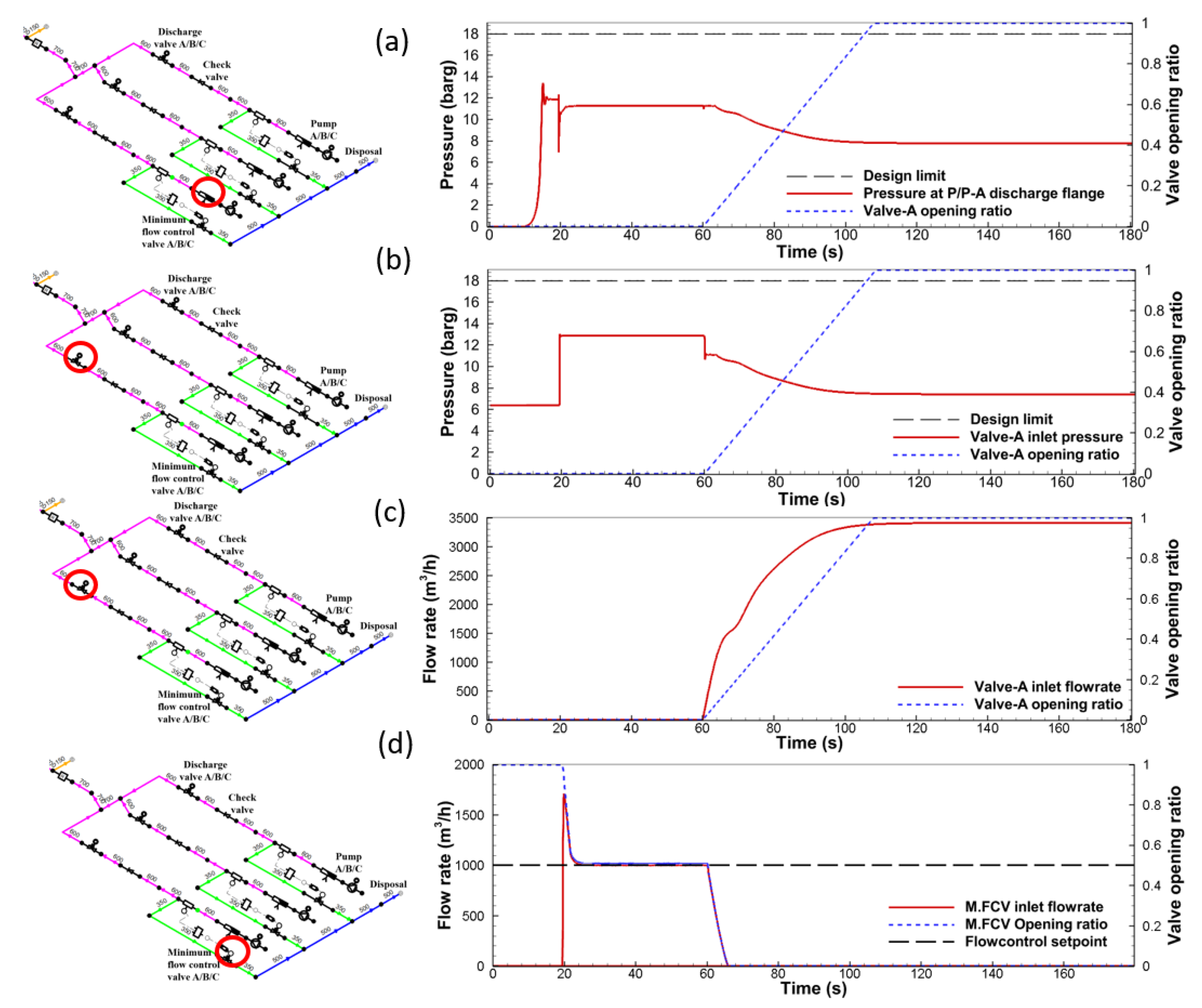
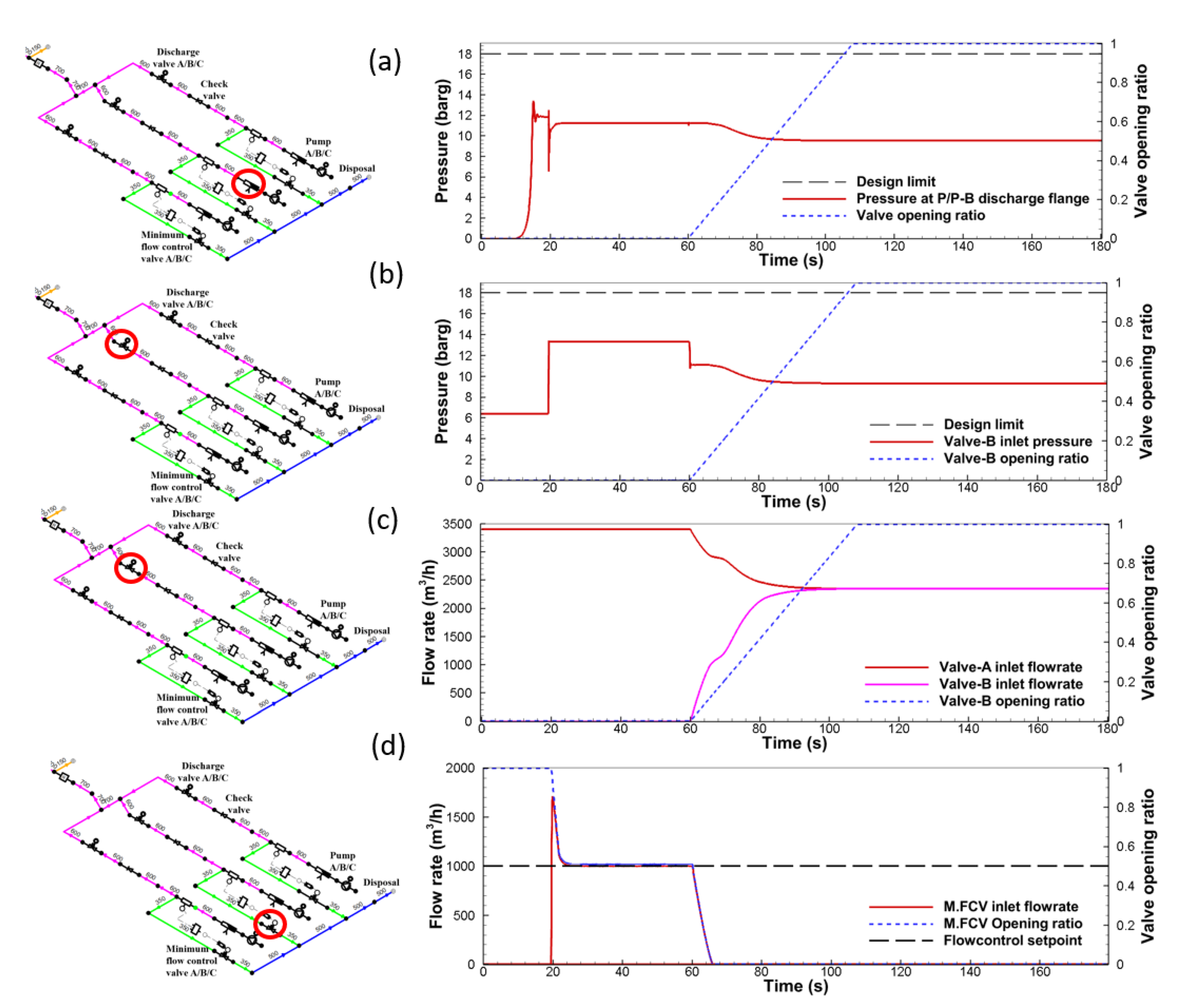
5.1. Result of Scenario 1: Pump A Start-Up Followed by Pump B Start-Up

Figure 13 and Figure 14 show the results of Scenario 1. A few seconds after pump A started, a slight pressure increase occurred at the pump discharge flange (Figure 13a) and the inlet to the discharge valve (Figure 13b), but this pressure was less than the design pressure. Discharge valve A opens after 60 s, and the flow rate was generated, and it was observed that the flow rate stabilized in steady state flow (Figure 13c). The minimum flow control valve A maintained the set 1000 m³/h while the valve opening was adjusted (Figure 13d). Figure 14a,b and d show that the start-up of pump B was similar to the start-up of pump A. As soon as the discharge valve B was opened at 60 s, the flow rate through it increased, while the flow rate through discharge valve A began to decrease (Figure 14c). With discharge valve B fully open, the flow rates in both valves became almost equal, and the total required flow rate of 4700 m³/h was attained.

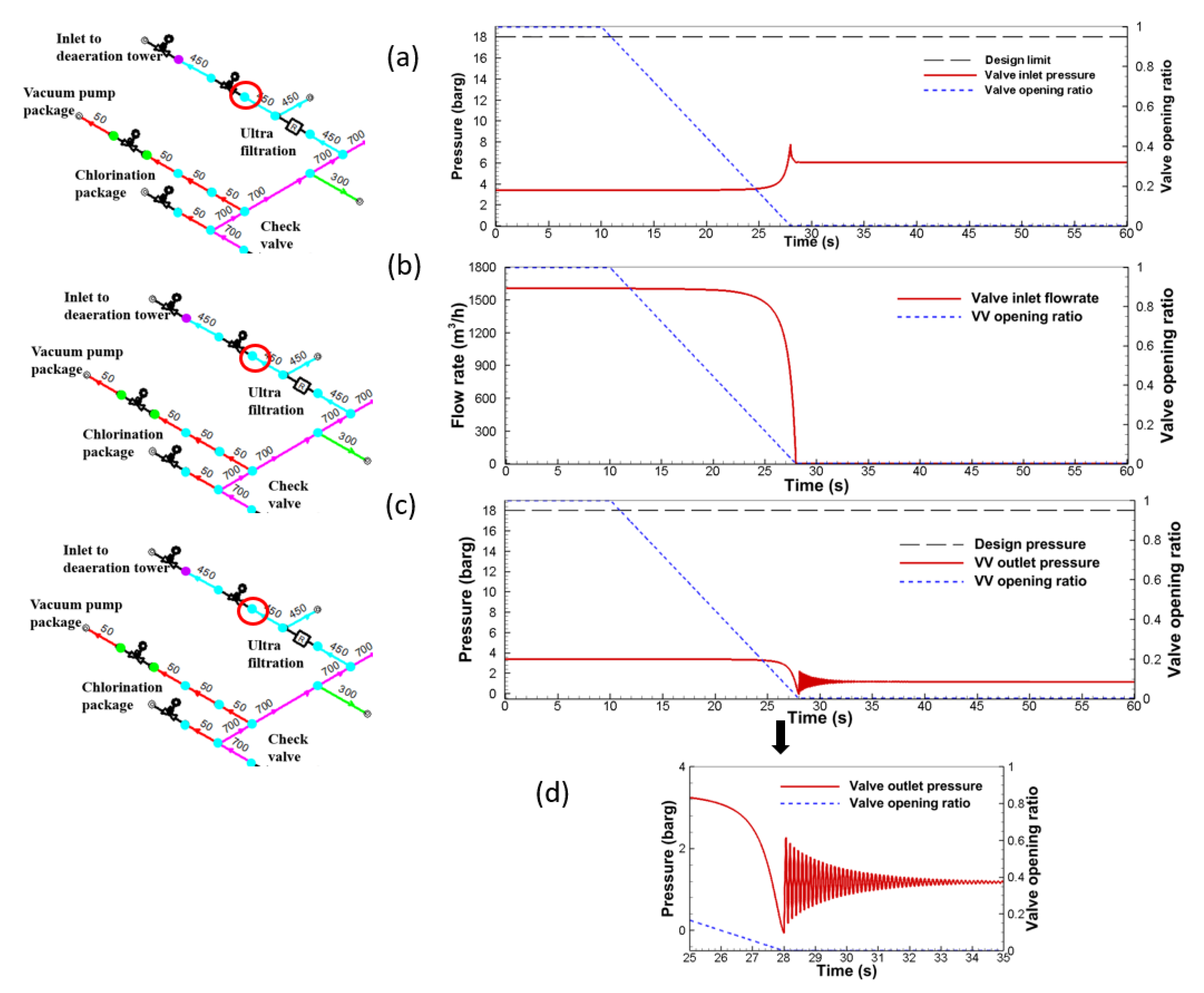
5.2. Result of Scenario 2: Valve Closure—Deaeration Tower Inlet

As soon as the valve was completely closed at 28 s, a slight increase in pressure occurred on the valve inlet side, but it was lower than the design pressure and it became stabilized again (Figure 15a). Figure 15b shows the sudden change in flow rate at 28 s when the valve is closed. Figure 15c,d show that a significant decrease in pressure caused the oscillation of the pressure on the valve outlet side. It seems that air pockets might have been entrapped at the valve outlet when the valve was rapidly closed, and they started to be compressed and oscillate as the fluid propagated.

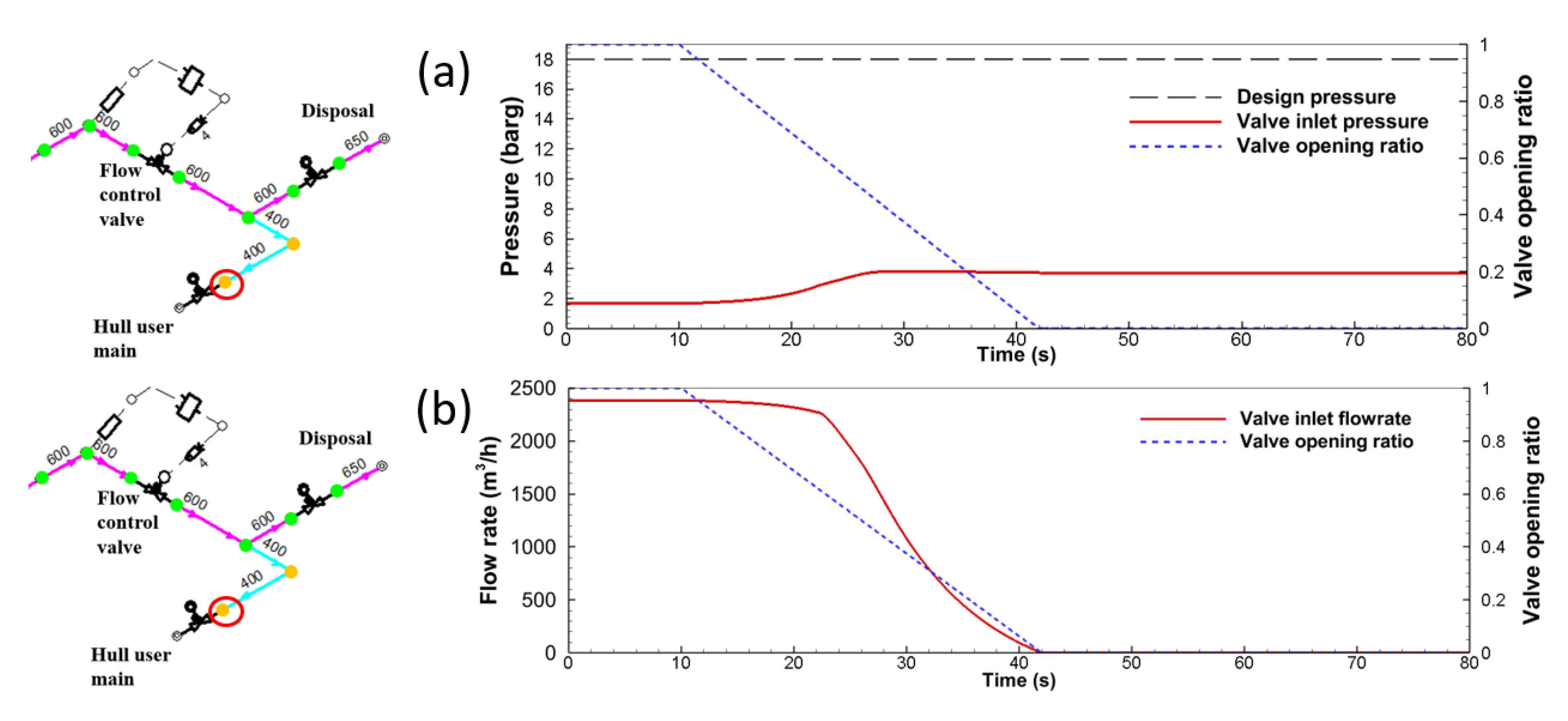
5.3. Result of Scenario 3: Valve Closure—Hull Seawater System Inlet

Figure 16 shows that, in this scenario, no noticeable pressure increases (Figure 16a) or oscillations in flow rate (Figure 16b) were observed. Since another much bigger branch for pipe disposal allows a continuous flow rate, less pressure rise at the hull service water branch was expected, which was smaller than the branch to the disposal pipe distance.

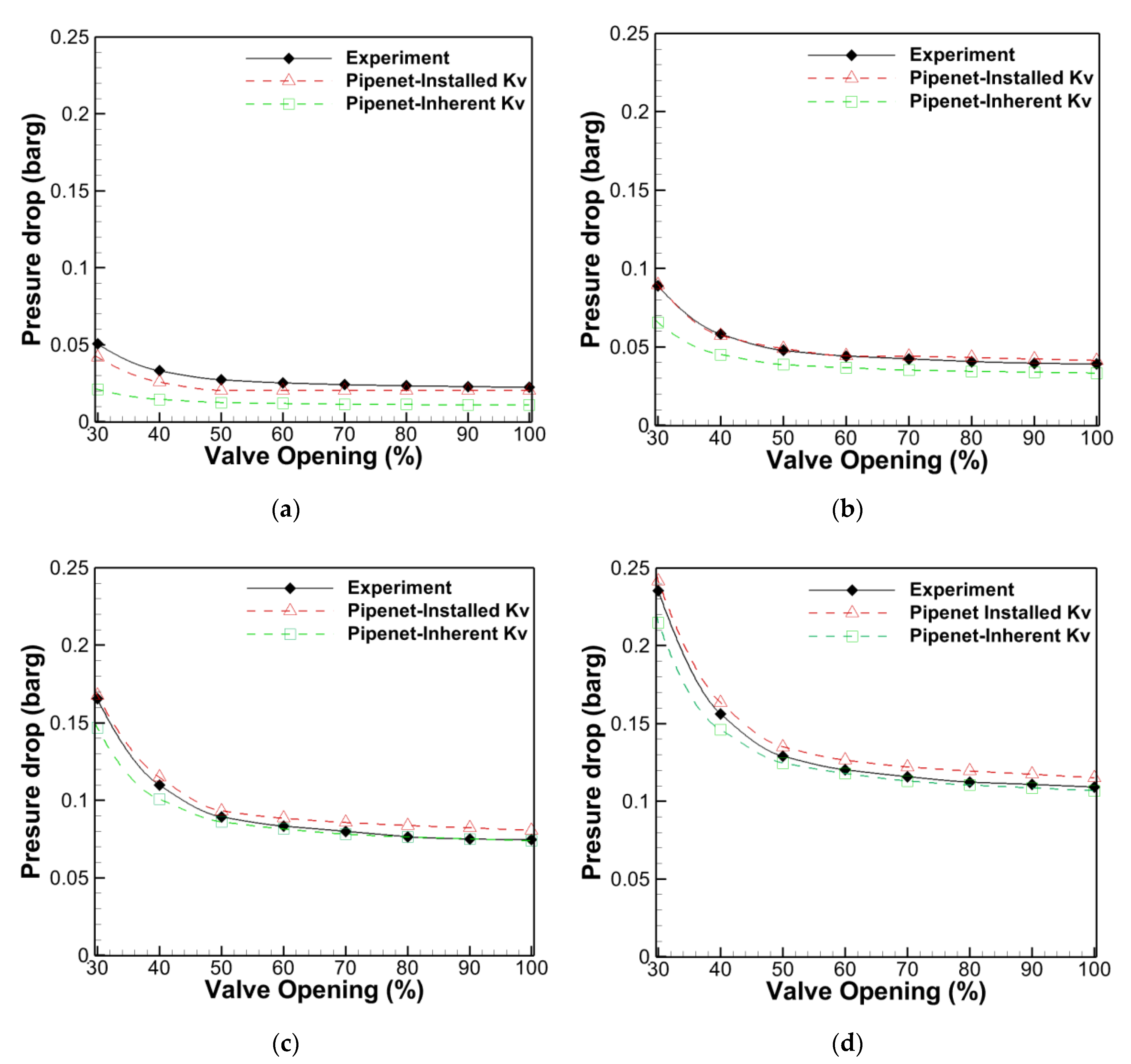
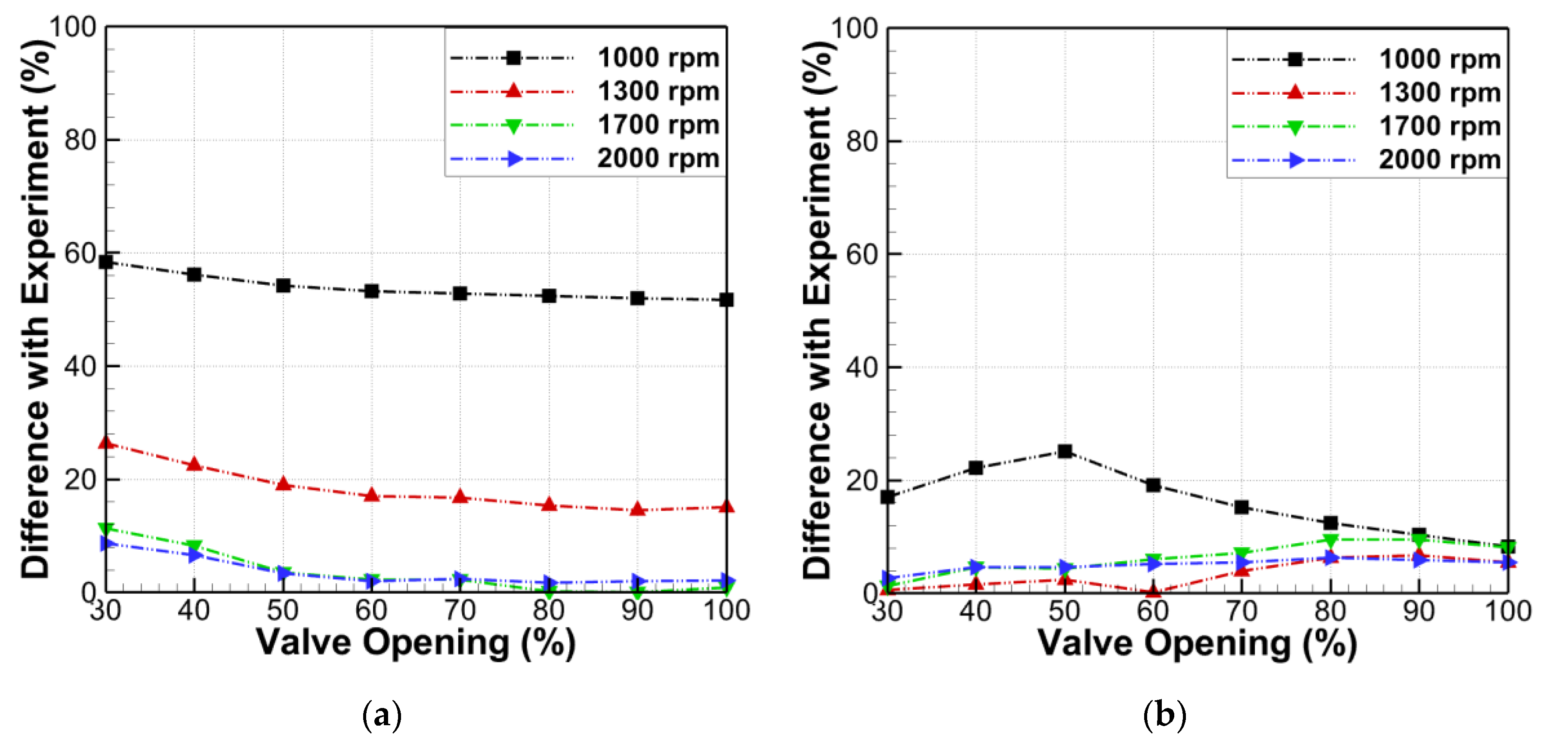
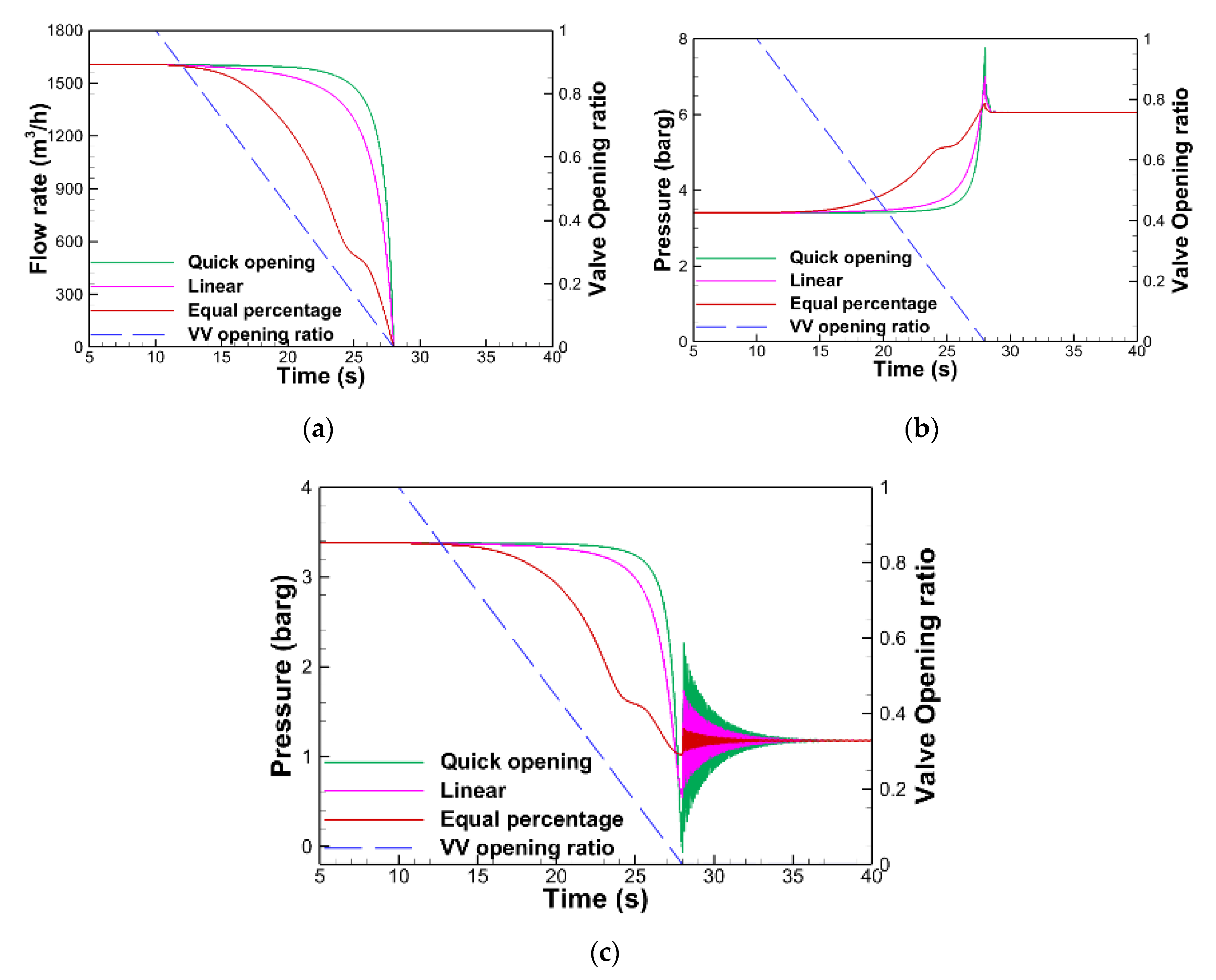
5.4. Effect of Valve Flow Characteristics

Figure 17a shows the change in flow rate with time when the valve is closed. Figure 17b,c show that the increase in the pressure at the inlet to the valve and the amplitude of the pressure oscillation of the outlet from the valve were much lower, i.e., approximately 1–1.8 barg, when using equal percentage valve flow characteristics. As confirmed in the parametric study, the type of valve used in the quick opening profile, such as the gate valve, has been found to be disadvantageous in terms of pressure surges. However, a butterfly valve with equal percentage flow characteristics is considered to be a more suitable type of valve when considering the water hammer phenomenon, since it allows a uniform flowrate during the opening and closing of the valve. In addition, since larger pipes are used in seawater treatment systems, the butterfly valve was found to be advantageous in terms of price because it weighed less than the gate valve. Figure 18 compares the weights gate valve and the butterfly valve. For 18′′ class 150, approximately a 50% weight reduction is expected.

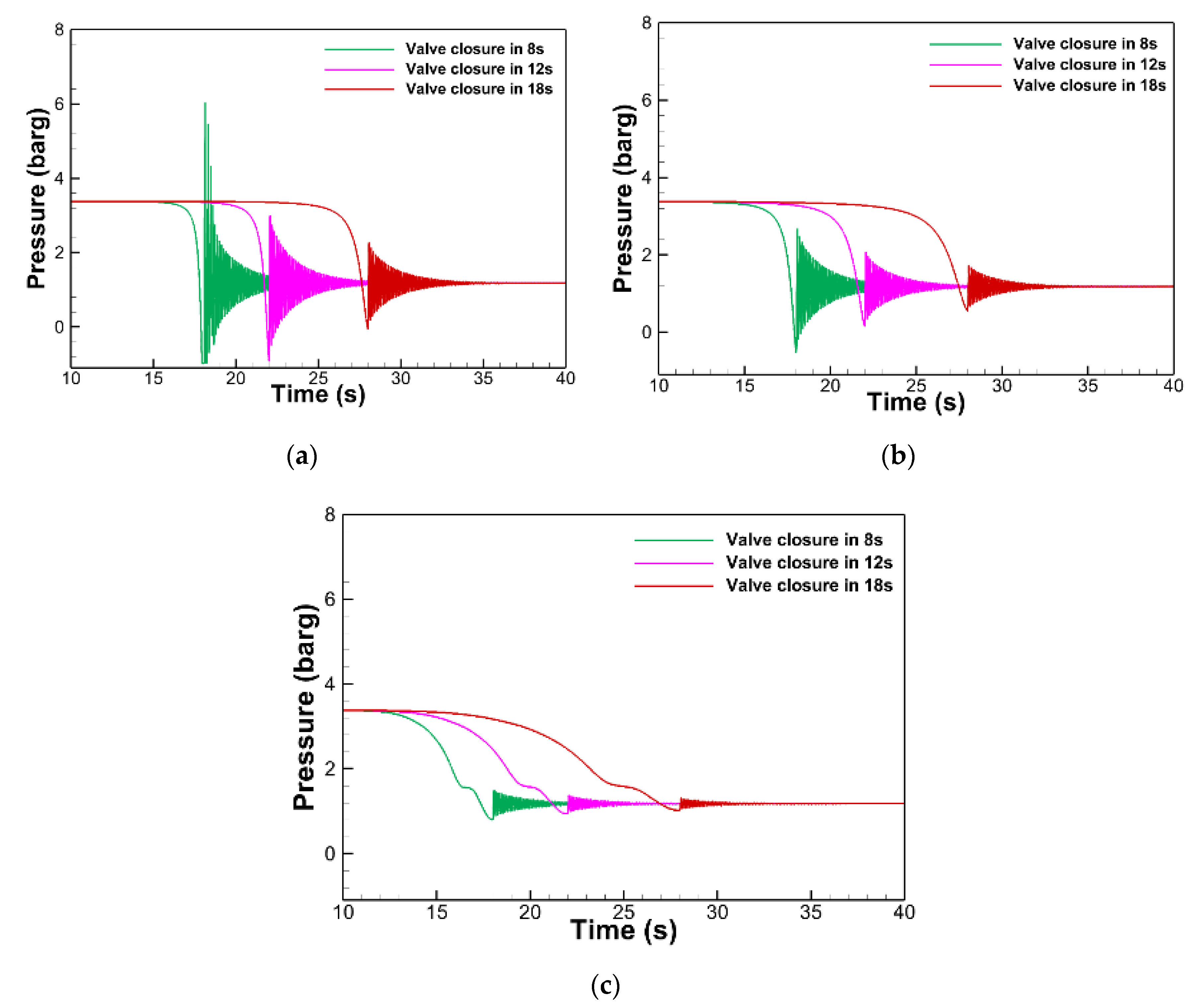
5.5. Effect of Valve Closure Time

In the case of the flow characteristics of quick opening valves, Figure 19a shows that a significant increase in pressure occurs after a sudden pressure drop if the valve is closed within 8 s. However, much smaller pressure fluctuations were observed when either a linear valve (Figure 19b) or an equal-percentage valve (Figure 19c) was used. The equal-percentage valve produced negligible oscillation in pressure even if the valve was closed within 8 s.

6. Conclusions

In this study, the dynamic responses of water hammer phenomenon were investigated in the seawater treatment system by a 1D simulation model approach based on the method of characteristics. The 1D simulation tools for both steady-state and unsteady-state analyses were validated by comparing the results with the experimental results. Case study with the extensive scenario on the defined piping network was performed to evaluate the effect of the valve closure time and valve flow characteristics. As a follow-up action in the case study, measures to reduce the water hammer phenomenon were proposed.

The key findings were summarized as follows:

• The 1D simulation model based on MOC could predict the pressure drop through the valve well using the inherent flow coefficient at a high Reynold number. If the installed flow coefficient could be provided for the real piping system, the results might be more accurate for whole regions of the pump speed. Furthermore, the simulation could estimate the surge pressure well until at least the second pressure peak. Moreover, this model with its quasi-steady friction term is likely to efficiently evaluate the maximum surge pressure caused by water hammer.
• The case study was performed for various scenarios of pump start-up and valve closure in the seawater treatment system. In the case of pump start-up (Case 1), a slight pressure increase was observed at the inlet of the discharge valve, but the predicted pressure was lower than the design pressure of the pipe. When the valve at the system inlet closed (Case 3), noticeable pressure increases did not occur because another branch of disposal pipe allowed the flow rate.
• However, pressure oscillations were observed downstream from the valve when the valve of the inlet part closed (Case 2). The pressure oscillation might be caused by air pockets entrapped at the valve outlet when the valve was rapidly closed. The amplitude of the oscillation was less than the design pressure of the piping system, but it may cause a severe damage to the system by vibration or making the flow efficiency worse.
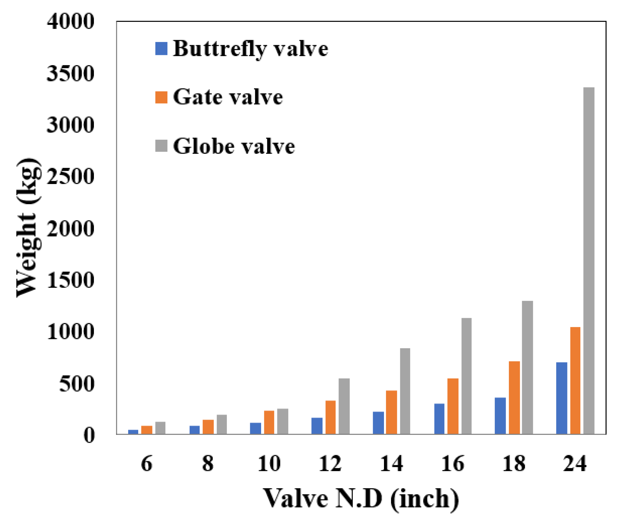
• To mitigate the pressure oscillation and improve the efficiency of the seawater treatment system, it is suggested to use a butterfly valve with equal percentage flow characteristic. Based on the comparison study with the gate valve (quick opening characteristic) and globe valve (linear characteristic), the advantages of using the butterfly valve can be followed:
  • Reducing the pressure surge and amplitude by 1–1.8 barg;
  • Allowing a 10 s decrease in the valve closure time;
  • Reducing the weight of valve by 50% in consideration with the dynamic effect of the piping structure.

References

1. Walters, T.W.; Leishear, R.A. When the Joukowsky Equation Does Not Predict Maximum Water Hammer Pressures. In Proceedings of the ASME 2018 Pressure Vessels and Piping Conference, Prague, Czech, 15–20 July 2018. Abstract number PVP2018-84050. [Google Scholar]
2. Simpson, A.R. Large Water Hammer Pressures Due to Column Separation in Sloping Pipes. Ph.D. Thesis, Department of Civil Engineering, University of Michigan, Ann Arbor, MI, USA, 1986. [Google Scholar]
3. Simpson, A.R.; Bergant, A. Numerical comparison of pipe column separation models. J. Hydraul. Eng. 1994, 120, 361–377. [Google Scholar] [CrossRef] [Green Version]
4. Kwon, H.J. Analysis of Transient Flow in a Piping system. J. Civil Eng. 2007, 11, 209–214. [Google Scholar] [CrossRef]
5. Jinping, L.I.; Peng, W.; Jiandong, Y. CFD numerical simulation of water hammer in pipeline based on the Navier-Stokes equation. In Proceedings of the V European Conference on Computational Fluid Dynamics (ECCOMAS CFD), Lisbon, Portugal, 14–17 June 2010. [Google Scholar]
6. Martins, N.M.C.; Brunone, B.; Meniconi, S.; Ramos, H.M.; Covas, D.I.C. CFD and 1D approaches for the unsteady friction analysis of low Reynolds number turbulent flows. J. Hydraul. Eng. 2017, 143, 04017050. [Google Scholar] [CrossRef]
7. Mandair, S.; Karney, B.; Magnan, R.; Morissette, J.F. Comparing Pure CFD and 1-D Solvers for the Classic Water Hammer Models of a Pipe-Reservoir System. In Proceedings of the 1st International WDSA/CCWI 2018 Joint Conference, Kingston, ON, Canada, 23–25 July 2018. [Google Scholar]
8. Wang, C.; Nilsson, H.; Yang, J.; Petit, O. 1D–3D coupling for hydraulic system transient simulations. J.CPC 2017, 210, 1–9. [Google Scholar] [CrossRef]
9. Ghidaoui, M.; Zhao, M.; McInnis, D.; Axworthy, D. A Review of Water Hammer Theory and Practice. Appl. Mech. Rev 2005, 58, 49–76. [Google Scholar] [CrossRef]
10. Korteweg, D.J. Ueber die Fortpflanzungsgeschwindigkeit des Schalles in elastischen Röhren (“On the velocity of propagation of sound in elastic tubes.”). Ann. Phys. 1878, 241, 525–542. [Google Scholar] [CrossRef] [Green Version]
11. Vardy, A.E.; Hwang, K.L. A characteristics model of transient friction in pipes. J. Hydraul. Res. 1991, 29, 669–684. [Google Scholar] [CrossRef]
12. Daily, W.J.; Hankey, W.L.; Olive, R.W.; Jordaan, J.M. Resistance coefficients for accelerated and decelerated flows through smooth tubes and orifices. Trans. ASME 1956, 1071–1077. [Google Scholar]
13. Shuy, E. Wall shear stress in accelerating and decelerating turbulent pipe flows. J. Hydraul. Res. 1996, 34, 173–183. [Google Scholar] [CrossRef]
14. Brunone, B.; Golia, U.M.; Greco, M. Some remarks on the momentum equation for fast transients. In Proceedings of the International Meeting on Hydraulic Transients with Column Separation, Valenica, Spain, 4–6 September 1991; pp. 201–209. [Google Scholar]
15. Lister, M. The Numerical Solution of Hyperbolic Partial Defferential Equations by the Method of Characteristics; Wiley: New York, NY, USA, 1960; pp. 165–179. [Google Scholar]
16. Wylie, E.B.; Streeter, V.L. Fluid Transients in Systems, 1st ed.; Prentice Hall: Englewood Cliffs, NJ, USA, 1993. [Google Scholar]
17. PIPENET: Leading the Way in Fluid Flow Analysis. Available online: https://www.sunrise-sys.com/ (accessed on 20 July 2020).
18. Nguyen, Q.K.; Jung, K.H.; Lee, G.N.; Suh, S.B.; To, P. Experimental Study on Pressure Distribution and Flow Coefficient of Globe Valve. Processes 2020, 8, 875. [Google Scholar] [CrossRef]
19. Bergant, A.; Simpson, A.; Vitkovsky, J. Review of unsteady friction models in transient pipe flow. In Proceedings of the 9th International Meeting on the Behaviour of Hydraulic Machinery Under Steady Oscillatory Conditions, International Assocication of Hydraulic Research, Brno, Czech, 7–9 September 1999. [Google Scholar]
20. Colebrook, C.F.; Blench, T.; Chatley, H.; Essex, E.; Finniecome, J.; Lacey, G.; Macdonald, G. Turbulent flow in pipes, with particular reference to the transition region between the smooth and rough pipe laws. J. Inst. Civil Eng. 1939, 12, 393–422. [Google Scholar] [CrossRef]
21. FloMASTER: Fluid Thinking for Systems Engineers. Available online: https://www.mentor.com/products/mechanical/flomaster/flomaster/ (accessed on 20 July 2020).
22. Mahgerefteh, H.; Rykov, Y.; Denton, G. Courant, Friedrichs and Lewy (CFL) impact on numerical convergence of highly transient flows. Chem. Eng. Sci. 2009, 64, 4969–4975. [Google Scholar] [CrossRef]
Figure 1. Method of characteristics grid.
Processes 08 01041 g001
Figure 2. Two-phase (air–water) flow loop in Pusan National University: (a) flow loop facilities; and (b) 3D model.
Processes 08 01041 g002
Figure 3. Performance of the pump.
Processes 08 01041 g003
Figure 4. Valve flow coefficient.
Processes 08 01041 g004
Figure 5. Schematic diagram of flow loop in PIPENET.
Processes 08 01041 g005
Figure 6. Effect of the flow coefficient on the pressure drop: (a) 1000 rpm; (b) 1300 rpm; (c) 1700 rpm; and (d) 2000 rpm.
Processes 08 01041 g006
Figure 7. Differences of the pressure drop between the simulation and experimental results: (a) inherent flow coefficient; and (b) installed flow coefficient.
Processes 08 01041 g007
Figure 8. Schematic diagram of the simulation set up: (a) FLOWMASTER; (b) PIPENET.
Processes 08 01041 g008
Figure 9. Comparison between the experimental and simulation results: (a) V = 0.1 m/s; (b) V = 0.2 m/s; and (c) V = 0.3 m/s.
Processes 08 01041 g009
Figure 10. Block flow diagram of the seawater treatment system.
Processes 08 01041 g010
Figure 11. Schematic diagram of the model in PIPENET.
Processes 08 01041 g011
Figure 12. Flow characteristics of different valves.
Processes 08 01041 g012
Figure 13. Pressure and flow rate change over the time history Scenario 1 pump A start-up: (a) pressure at discharge flange of pump A; (b) Pressure at the inlet of the discharge valve; (c) flow rate at the inlet of the flange of pump A; (b) pressure at the inlet of the discharge valve; (c) flow rate at the inlet of the discharge valve A; (d) flow rate at the inlet of minimum flow control valve A.
Processes 08 01041 g013
Figure 14. Changes in the pressure and flow rate over time history Scenario 1 Pump B start-up: (a) Pressure at the discharge flange of pump B; (b) pressure at the discharge valve B inlet; (c) flow rate at discharge valve B inlet; and (d) the flow rate at the minimum flow control valve B inlet.
Processes 08 01041 g014
Figure 15. Changes in the pressure and flow rate over time (Scenario 2): (a) valve inlet pressure; (b) valve inlet flow rate; (c) valve outlet pressure; (d) zoom-in of pressure oscillation.
Processes 08 01041 g015
Figure 16. Pressure and flow rate change over time history Scenario 3: (a) valve inlet pressure; and (b) valve inlet flow rate.
Processes 08 01041 g016
Figure 17. Effect of valve flow characteristics: (a) Flow rate; (b) Pressure at the inlet of the valve; (c) Pressure at outlet of the valve.
Processes 08 01041 g017
Figure 18. Comparison of the weights of valves.
Processes 08 01041 g018
Figure 19. Effect of valve closing time: (a) quick opening characteristic; (b) linear characteristic; and (c) equal percentage characteristic.
Processes 08 01041 g019