The Role of Technological Innovation in a Dynamic Model of the Environmental Supply Chain Curve: Evidence from a Panel of 102 Countries

 , ,
, , 

 and
and
Abstract

1. Introduction
Contribution of the Study, Research Questions and Objectives of the Study
- (i)
- To examine the role of logistics performance indices in the cost of carbon emissions across countries.
- (ii)
- To investigate the dynamic linkages between technological factors and carbon damages in a panel of selected countries.
- (iii)
- To determine the potential impact of economic growth, industry value-added, medium and high-tech industry, and insurance and financial services on the cost of carbon emissions across countries, and
- (iv)
- To substantiate an inverted U-shaped relationship between carbon damages and economic growth, and carbon damages and technology-induced logistics performance indices across countries.
2. Materials and Methods
- (i)
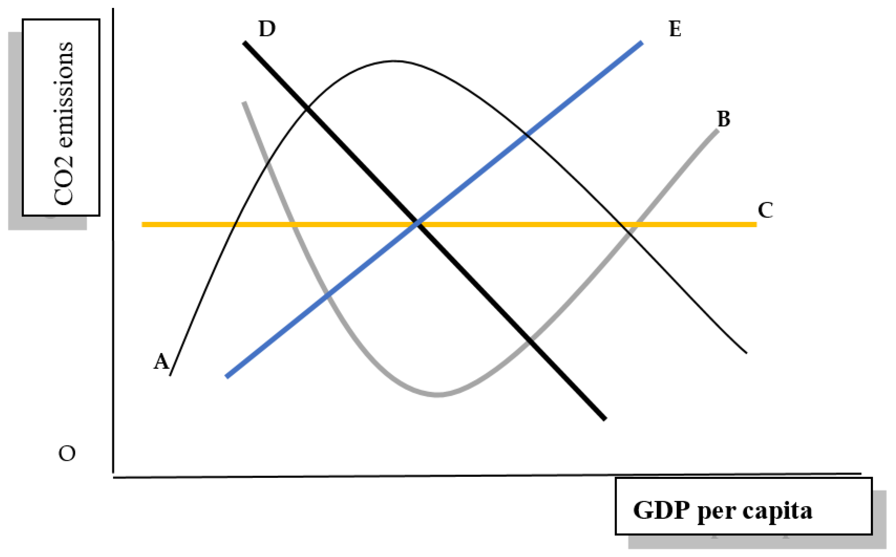
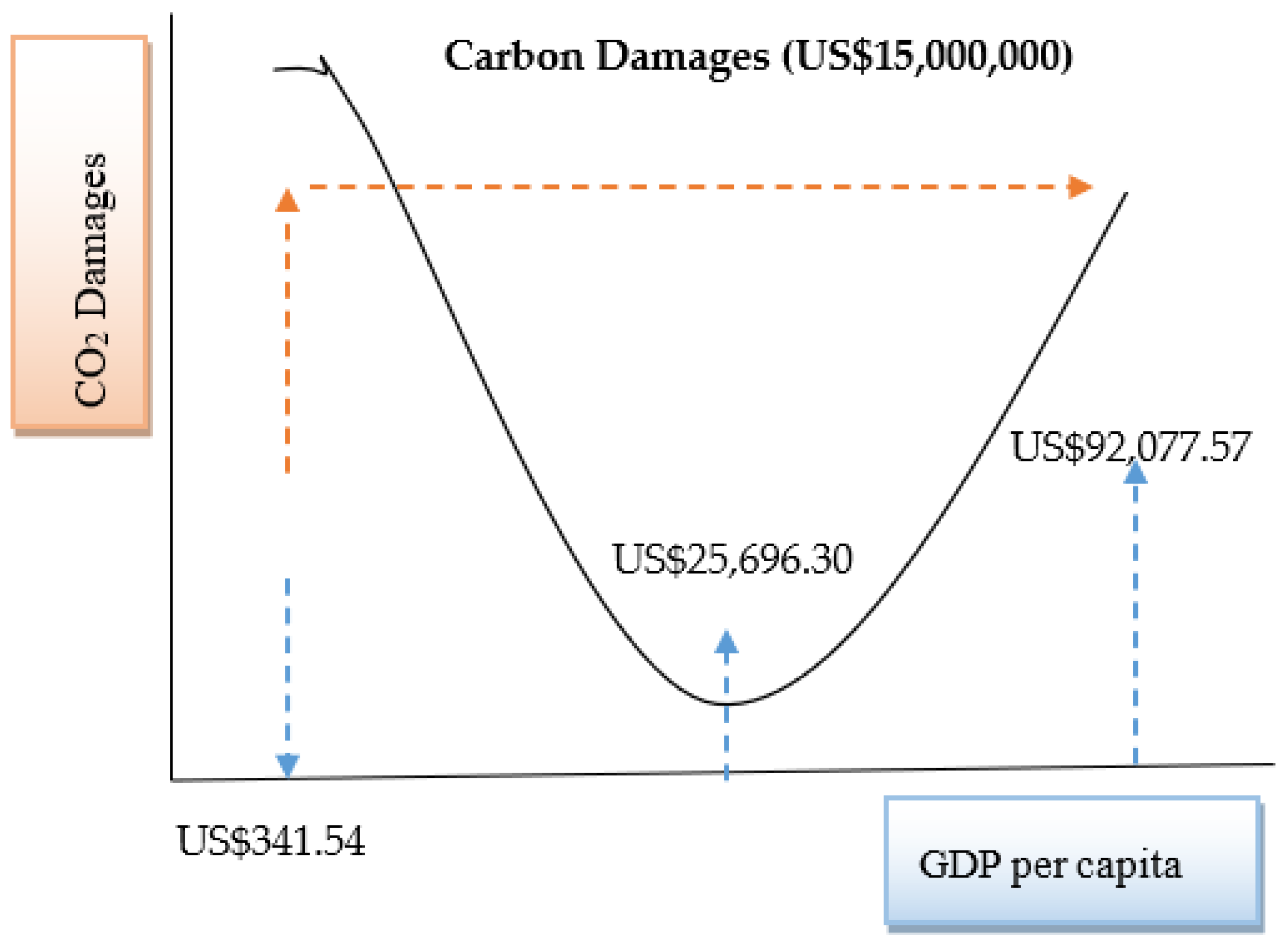
- Environmental Kuznets Curve (EKC): The EKC shows the non-linear relationship between income per capita and per capita carbon emissions at the second-degree quadratic version. The nominal GDP per capita and its second degree confined its positive and negative impact on carbon emissions, respectively, to substantiate an inverted U-shaped EKC hypothesis [47,48,49]. The other forms could also be found under different socio-economic and environmental factors across varied economic settings [50,51]. Figure 2 shows the five different possibilities of EKC hypotheses to clearly understand the given concept to use in a given study for more critical insights. Line A shows an inverted U-shaped relationship between the country’s income and carbon emissions, which first increases than decreases carbon emissions due to vital environmental reforms being done through the country’s economic growth. Line B shows the U-shaped relationship between the two stated factors that show carbon emissions decrease initially with the country’s economic growth that later increases due to high industrialization caused by continued economic growth. Line C shows the flat EKC hypothesis, which argued that both the variables have no relationship. Line D shows monotonic decreasing function, while line E shows the monotonic increasing function that shows only one portion of the EKC hypothesis, either from the right side or left side, while the latter is insignificant.
- (ii)
- Technology-Induced Emissions: Grossman and Krueger [52] explored three different economic effects on the environment, i.e., scale effects, technological effects, and composition effects. The combination of these scales would help support the EKC hypothesis, i.e., the rapid economic transformation would increase the country’s economies of scale that cause environmental degradation. Simultaneously, technological effects are most visible in developed countries that increase R & D expenditures to obsolete dirty polluting technologies and replace it with the cleaner technologies that ultimately affect the composition of production, which support the EKC hypothesis in a long-run. The less developed countries usually unscaled the dirty production due to easing environmental regulations, which ultimately increases carbon emissions.
- (iii)
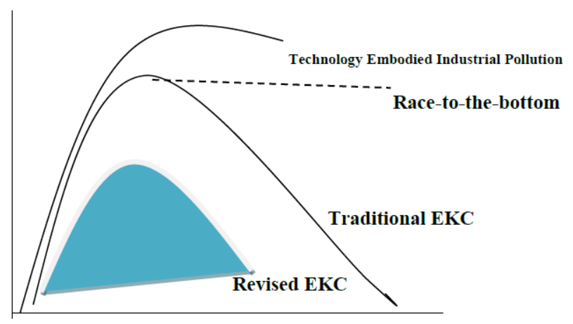
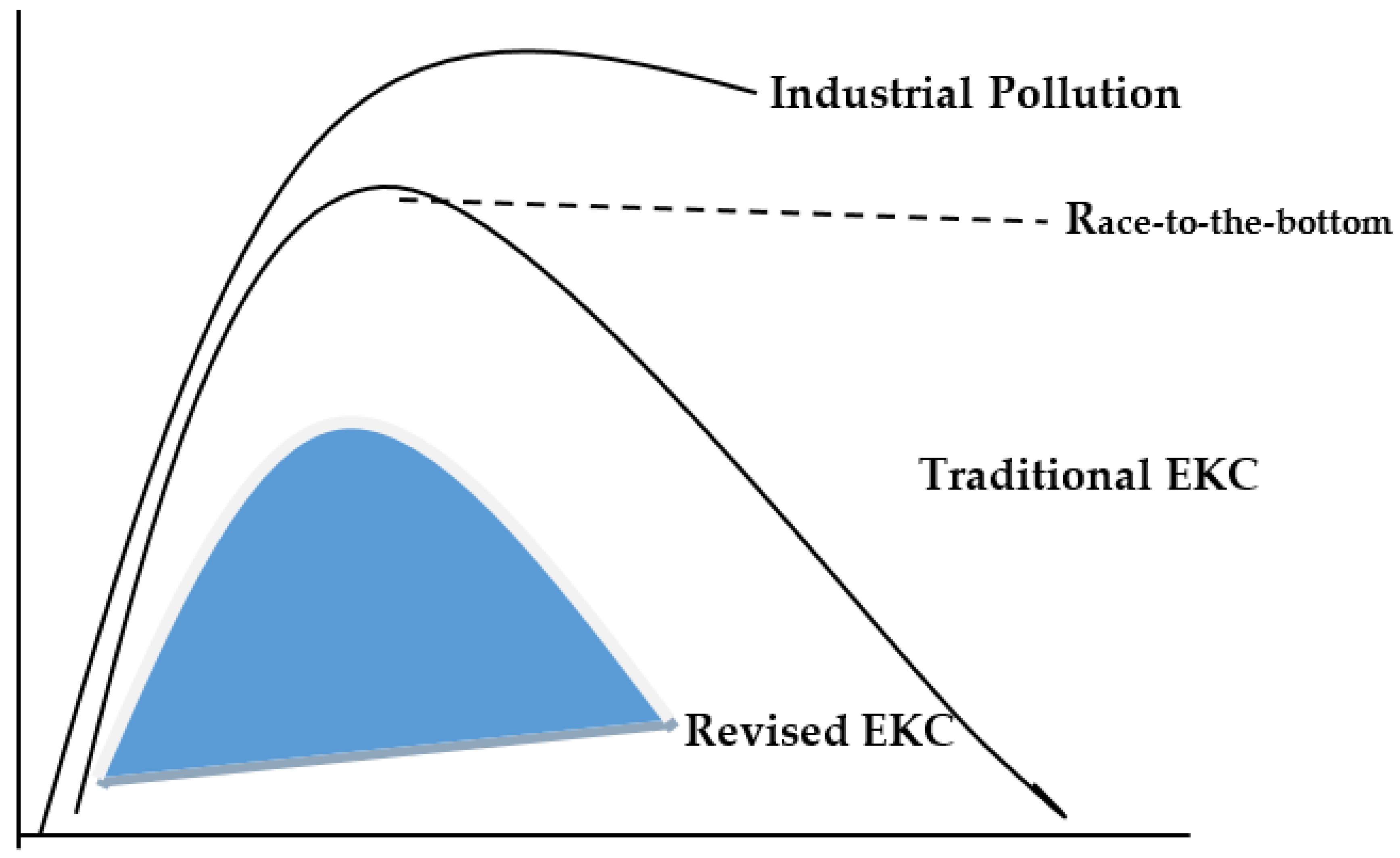
- New Toxic Pollutants, Race-to-the-Bottom Hypothesis, and Revised EKC Hypothesis: The rapid industrialization shifts country’s structural transmission mechanisms to using high-tech products that cause new toxic pollutants in the atmosphere, thus showing a single right-sided portion of EKC hypothesis. Further, due to developed countries’ stringent environmental regulations to restrain the polluting industries, the production units shift widely from developed to developing countries, thus showing the race-to-the-bottom hypothesis. Finally, due to technology infusion and broadcasting, environmental awareness programs burden less developed countries to limit carbon emissions through fewer resources. Thus, the EKC hypothesis’s kurtosis and its diameter fall short of the conventional EKC hypothesis (see Figure 3).
- (iv)
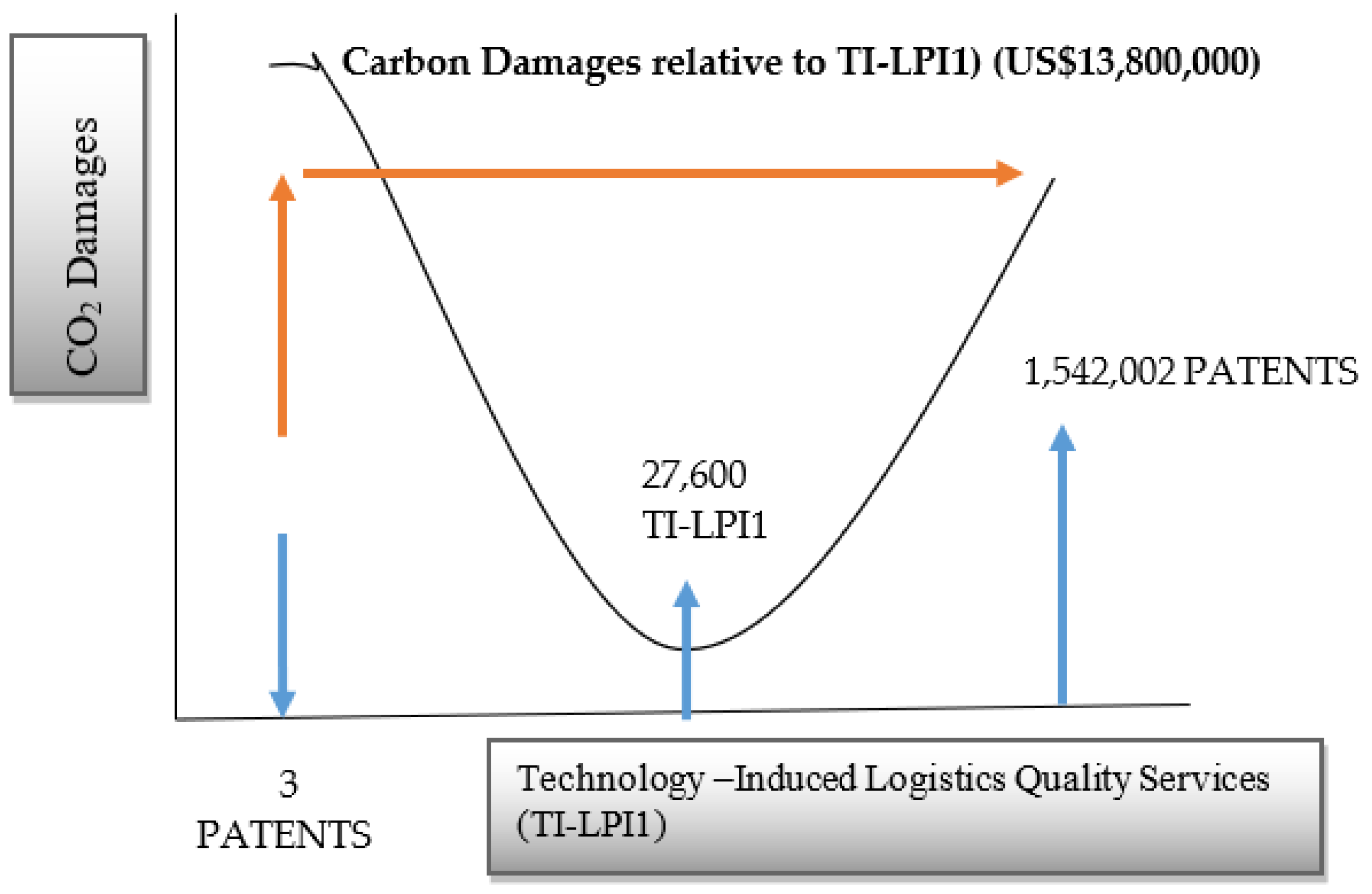
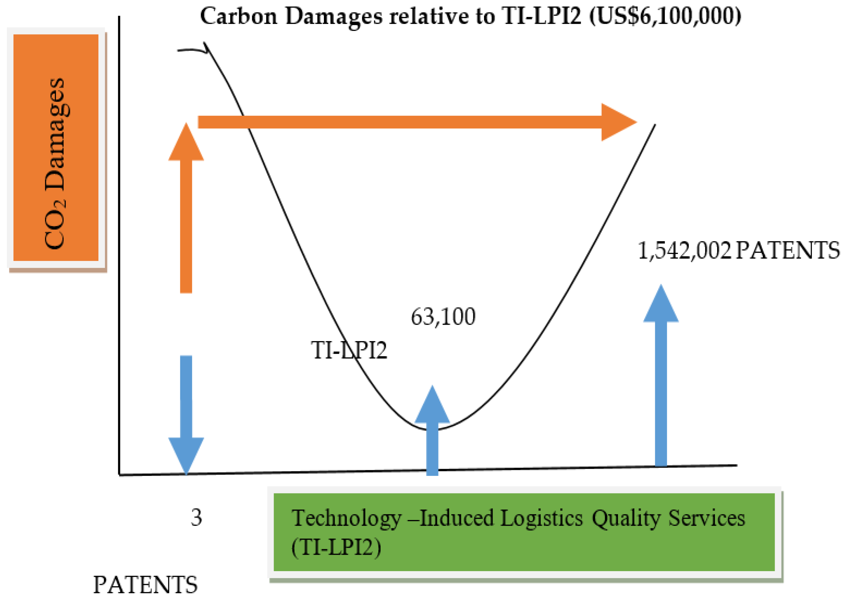
- Green Supply Chain Management Process (GSCMP): The discussion of the EKC hypothesis is carried forward under logistics operations, which are embodied with technological progress to make an intelligent machine design fuel-efficient and advanced for smart and green production. It is expected that with the moderation of technical factors with logistics performance indices would make a green supply chain process that would be less sensitive to carbon emissions. Thus, it would form different possibilities of the EKC hypothesis across countries.
2.1. Theoretical and Econometric Framework
Prevention of Losses/Gains from CDAM = Cost of Carbon Emissions in US$ − Minimum Value of CDAM in US$)
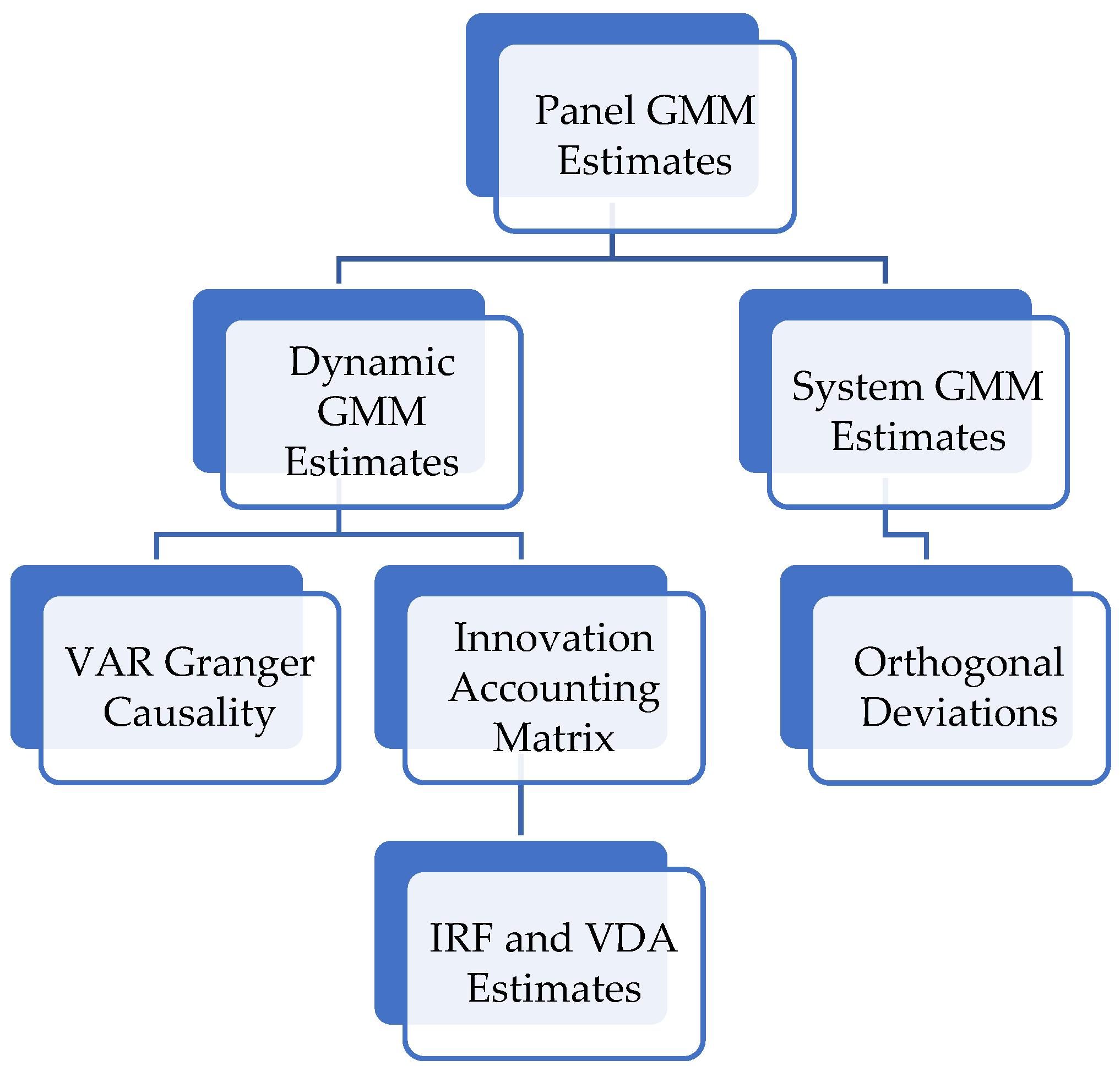
2.2. Research Methods
- (i)
- It works under large cross-sections and limited time. In this study, there are 102 countries in a panel setting with a period of the last nine years.
- (ii)
- It handles more than one endogenous issue in the given models. The current study used simultaneous equations modeling; thus the chances of any known endogenous issue may mislead the model. Therefore, for the results’ soundness, the differenced GMM estimator is good enough to observe this issue by including lagged instrumental variables.
- (iii)
- The problem of autocorrelation in panel settings might get affected by the studied parameter estimates. Thus, AR(1) and AR(2) would perform diagnostic tests to check any possible autocorrelation issues. If AR(1) does not fall in the 5% confidence interval, while AR(2) appears at a 5% significance level, the problem of autocorrelation problem would be resolved.
- (iv)
- The differenced GMM estimator is based upon the two-step procedure. In the first step, the regression is performed at differenced level, while in the second step, the lagged dependent variable included as a regressor in the given equations to remove simultaneity issues, and
- (v)
- The J-statistic and instrumental rank would be assessed to check the reliability of using given instruments as a true estimator in the given equations.
- -
- Whether LPIs (and technological factors, and growth-specific factors) Granger cause carbon damages, and simultaneously whether carbon damages Granger cause LPIs (and technical factors, and growth-specific factors)? If both conditions hold, then the given relationship would be bidirectional in nature.
- -
- Whether LPIs (and technological factors, and growth-specific factors) Granger cause carbon damages? The reverse does not hold the causal relationship, thus the given link would be unidirectional in nature.
- -
- Whether carbon damages Granger cause LPIs (and technological factors and growth-specific factors)? If the reverse does not hold the same then the given relationship would be one-directional in nature.
- -
- Whether LPIs (and technological factors, and growth-specific factors) do not Granger cause carbon damages, and simultaneously whether carbon damages do not Granger cause LPIs (and technical factors, and growth-specific factors)? In this case there will be no causal relationship between the stated variables.
- (i)
- To evaluate the relationship between the stated variables in inter-temporal settings.
- (ii)
- To assess the magnitude and direction between the variables over a time horizon.
- (iii)
- To check one standard error shock on the exogenous variables over the endogenous variable.
- (iv)
- These techniques would be desirable to get robust parameter estimates, which would further help devise policy implications.
3. Results
- (i)
- Logistics activities, technical factors, and growth-specific factors are considered the chief source to increase carbon damages across countries.
- (ii)
- The performance of logistics activities depends upon the country’s financial ability and technological capabilities.
- (iii)
- Country’s economic growth depends upon advancement in the technical factors and insurance and financial services in a panel of selected countries.
4. Conclusions
- Advancement in cleaner production technologies is imperative to reduce the cost of carbon emissions across countries.
- Fuel efficient technologies can be used in logistics operations to improve quality services.
- Logistics operations should be diversified and compliant with all environmental regulations, including ISO-based environmental certifications, ISO certifications for efficient manufacturing units processing, ISO standardization certifications, and ISO certification for clean vehicle transportations.
- Insurance and financial services could expand business opportunities and manufacturers’ payoff by transporting their shipments from one place to another place, while the theft and other damages could be covered by efficient insurance services. Financial services’ soundness would also create a strong liaison between the financial market and investors to decide on smart production. Hence the process of green supply chain management would be enhanced with technical expertise.
- The cost of carbon emissions is further reduced by sustainable production decisions and high-tech productions, which is a way forward for smart production systems.
Author Contributions
Funding
Conflicts of Interest
Appendix A

| “Albania, Algeria, Argentina, Armenia, Australia, Austria, Azerbaijan, Bahrain, Bangladesh, Belarus, Belgium, Bolivia, Bosnia and Herzegovina, Botswana, Brazil, Bulgaria, Cambodia, Canada, Chile, China, Colombia, Costa Rica, Croatia, Cyprus, Czech Republic, Ecuador, Egypt, El Salvador, Estonia, Ethiopia, Finland, France, Georgia, Germany, Greece, Guatemala, Haiti, Honduras, Hong Kong, Hungary, Iceland, India, Indonesia, Italy, Jamaica, Japan, Jordan, Kazakhstan, Kenya, Korea, Kyrgyz Republic, Lao PDR, Latvia, Lebanon, Lithuania, Madagascar, Malaysia, Malta, Mauritius, Mexico, Moldova, Mongolia, Montenegro, Morocco, Mozambique, Namibia, Nepal, Nigeria, North Macedonia, Norway, Oman, Pakistan, Panama, Peru, Philippines, Poland, Portugal, Qatar, Romania, Russia, Rwanda, Saudi Arabia, Serbia, Singapore, Slovak Republic, Slovenia, South Africa, Spain, Sri Lanka, Sweden, Switzerland, Thailand, Trinidad and Tobago, Tunisia, Turkey, Ukraine, United Kingdom, United States, Uruguay, Venezuela RB, Zambia”. |
References
- United Nation. Sustainable Development Goals. 2015. Available online: https://sustainabledevelopment.un.org/?menu=1300 (accessed on 21 April 2020).
- Zand, F.; Yaghoubi, S.; Sadjadi, S.J. Impacts of government direct limitation on pricing, greening activities and recycling management in an online to offline closed loop supply chain. J. Clean. Prod. 2019, 215, 1327–1340. [Google Scholar] [CrossRef]
- Van Wassenhove, L.N. Sustainable innovation: Pushing the boundaries of traditional operations management. Prod. Oper. Manag. 2019, 28, 2930–2945. [Google Scholar] [CrossRef]
- Marsden, T.; Rucinska, K. After COP21: Contested transformations in the energy/agri-food nexus. Sustainability 2019, 11, 1695. [Google Scholar] [CrossRef]
- Evans, S.; Gabbatis, J. COP25: Key Outcomes Agreed at the UN Climate Talks in Madrid, 2019. COP25 Madrid, 15th December 2019. Available online: https://www.carbonbrief.org/cop25-key-outcomes-agreed-at-the-un-climate-talks-in-madrid (accessed on 2 August 2020).
- World Bank. Aggregated LPI 2012–2018. 2019. Available online: https://lpi.worldbank.org/international/aggregated-ranking (accessed on 21 April 2020).
- WIPO. WIPO IP Facts and Figures 2018; World Intellectual Property Organization: Geneva, Switzerland, 2018. [Google Scholar]
- Avgerou, C. The link between ICT and economic growth in the discourse of development. In Organizational Information Systems in the Context of Globalization; Springer: Boston, MA, USA, 2003; pp. 373–386. [Google Scholar]
- Jungmittag, A. Innovations, technological specialisation and economic growth in the EU. Int. J. Econ. Policy 2004, 1, 247–273. [Google Scholar] [CrossRef]
- Mokyr, J. Long-term economic growth and the history of technology. In Handbook of Economic Growth; Elsevier: Amsterdam, The Netherlands, 2005; Volume 1, pp. 1113–1180. [Google Scholar]
- Smith, S.; Newhouse, J.P.; Freeland, M.S. Income, insurance, and technology: Why does health spending outpace economic growth? Health Aff. 2009, 28, 1276–1284. [Google Scholar] [CrossRef] [PubMed]
- Prieto, L. Innovation and Economic Growth: Cross-Country Analysis using Science and Technology Indicators. Ph.D. Thesis, Georgetown University, Washington, DC, USA, April 2017. [Google Scholar]
- Khan, H.U.R.; Zaman, K.; Khan, A.; Islam, T. Quadrilateral relationship between information and communications technology, patent applications, research and development expenditures, and growth factors: Evidence from the group of seven (G-7) countries. Soc. Indic. Res. 2017, 133, 1165–1191. [Google Scholar] [CrossRef]
- Irandoust, M. The renewable energy-growth nexus with carbon emissions and technological innovation: Evidence from the Nordic countries. Ecol. Indic. 2016, 69, 118–125. [Google Scholar] [CrossRef]
- Wang, M.; Feng, C. Decoupling economic growth from carbon dioxide emissions in China’s metal industrial sectors: A technological and efficiency perspective. Sci. Total Environ. 2019, 691, 1173–1181. [Google Scholar] [CrossRef]
- Demartini, M.; Pinna, C.; Aliakbarian, B.; Tonelli, F.; Terzi, S. Soft drink supply chain sustainability: A case based approach to identify and explain best practices and key performance indicators. Sustainability 2018, 10, 3540. [Google Scholar] [CrossRef]
- Mastos, T.D.; Nizamis, A.; Vafeiadis, T.; Alexopoulos, N.; Ntinas, C.; Gkortzis, D.; Papadopoulos, A.; Ioannidis, D.; Tzovaras, D. Industry 4.0 sustainable supply chains: An application of an IoT enabled scrap metal management solution. J. Clean. Prod. 2020, 269, 122377. [Google Scholar] [CrossRef]
- Kolhe, M.L.; Labhasetwar, P.K.; Suryawanshi, H.M. Smart Technologies for Energy, Environment and Sustainable Development: Select Proceedings of ICSTEESD 2018; Springer: Berlin, Germany, 2019. [Google Scholar]
- Dyczkowska, J.; Reshetnikova, O. New Technological Solutions in Logistics on the Example of Logistics Operators in Poland and Ukraine. In SMART Supply Network; Springer: Cham, Switzerland, 2019; pp. 47–69. [Google Scholar]
- Wang, Y.; Ren, H.; Dong, L.; Park, H.S.; Zhang, Y.; Xu, Y. Smart solutions shape for sustainable low-carbon future: A review on smart cities and industrial parks in China. Technol. Forecast. Soc. Chang. 2019, 144, 103–117. [Google Scholar] [CrossRef]
- Zaman, K.; Shamsuddin, S. Green logistics and national scale economic indicators: Evidence from a panel of selected European countries. J. Clean. Prod. 2017, 143, 51–63. [Google Scholar] [CrossRef]
- Khan, S.A.R.; Qianli, D. Does national scale economic and environmental indicators spur logistics performance? Evidence from UK. Environ. Sci. Pollut. Res. 2017, 24, 26692–26705. [Google Scholar] [CrossRef]
- Zaman, K. The impact of hydro-biofuel-wind energy consumption on environmental cost of doing business in a panel of BRICS countries: Evidence from three-stage least squares estimator. Environ. Sci. Pollut. Res. 2018, 25, 4479–4490. [Google Scholar] [CrossRef] [PubMed]
- Yu, Z.; Golpîra, H.; Khan, S.A.R. The relationship between green supply chain performance, energy demand, economic growth and environmental sustainability: An empirical evidence from developed countries. LogForum 2018, 14, 479–494. [Google Scholar] [CrossRef]
- Aldakhil, A.M.; Nassani, A.A.; Awan, U.; Abro, M.M.Q.; Zaman, K. Determinants of green logistics in BRICS countries: An integrated supply chain model for green business. J. Clean. Prod. 2018, 195, 861–868. [Google Scholar] [CrossRef]
- Liu, J.; Yuan, C.; Hafeez, M.; Yuan, Q. The relationship between environment and logistics performance: Evidence from Asian countries. J. Clean. Prod. 2018, 204, 282–291. [Google Scholar] [CrossRef]
- Khan, S.A.R.; Jian, C.; Zhang, Y.; Golpîra, H.; Kumar, A.; Sharif, A. Environmental, social and economic growth indicators spur logistics performance: From the perspective of South Asian Association for Regional Cooperation countries. J. Clean. Prod. 2019, 214, 1011–1023. [Google Scholar] [CrossRef]
- Liang, Z.; Chiu, Y.H.; Li, X.; Guo, Q.; Yun, Y. Study on the Effect of Environmental Regulation on the Green Total Factor Productivity of Logistics Industry from the Perspective of Low Carbon. Sustainability 2020, 12, 175. [Google Scholar] [CrossRef]
- Lan, S.; Tseng, M.L.; Yang, C.; Huisingh, D. Trends in sustainable logistics in major cities in China. Sci. Total Environ. 2020, 712, 136381. [Google Scholar] [CrossRef]
- Kumail, T.; Ali, W.; Sadiq, F.; Wu, D.; Aburumman, A. Dynamic linkages between tourism, technology and CO2 emissions in Pakistan. Anatolia 2020, 1–13. [Google Scholar] [CrossRef]
- Ahmad, M.; Khattak, S.I.; Khan, A.; Rahman, Z.U. Innovation, foreign direct investment (FDI), and the energy–pollution–growth nexus in OECD region: A simultaneous equation modeling approach. Environ. Ecol. Stat. 2020, 27, 203–232. [Google Scholar] [CrossRef]
- Ghazvini, M.; DehghaniMadvar, M.; Ahmadi, M.H.; Rezaei, M.H.; El Haj Assad, M.; Nabipour, N.; Kumar, R. Technological assessment and modeling of energy-related CO2 emissions for the G8 countries by using hybrid IWO algorithm based on SVM. Energy Sci. Eng. 2020, 8, 1285–1308. [Google Scholar] [CrossRef]
- Shahbaz, M.; Raghutla, C.; Song, M.; Zameer, H.; Jiao, Z. Public-private partnerships investment in energy as new determinant of CO2 emissions: The role of technological innovations in China. Energy Econ. 2020, 86, 104664. [Google Scholar] [CrossRef]
- Usman, O.; Olanipekun, I.O.; Iorember, P.T.; Abu-Goodman, M. Modelling environmental degradation in South Africa: The effects of energy consumption, democracy, and globalization using innovation accounting tests. Environ. Sci. Pollut. Res. 2020, 27, 8334–8349. [Google Scholar] [CrossRef]
- Khan, Z.; Hussain, M.; Shahbaz, M.; Yang, S.; Jiao, Z. Natural resource abundance, technological innovation, and human capital nexus with financial development: A case study of China. Resour. Policy 2020, 65, 101585. [Google Scholar] [CrossRef]
- Saleem, H.; Khan, M.B.; Shabbir, M.S. The role of financial development, energy demand, and technological change in environmental sustainability agenda: Evidence from selected Asian countries. Environ. Sci. Pollut. Res. 2020, 27, 5266–5280. [Google Scholar] [CrossRef]
- Azimi, M.; Feng, F.; Zhou, C. Environmental policy innovation in China and examining its dynamic relations with air pollution and economic growth using SEM panel data. Environ. Sci. Pollut. Res. 2020, 27, 9987–9998. [Google Scholar] [CrossRef]
- Ibrahiem, D.M. Do technological innovations and financial development improve environmental quality in Egypt? Environ. Sci. Pollut. Res. 2020, 27, 10869–10881. [Google Scholar] [CrossRef]
- Mariano, E.B.; Gobbo, J.A.; De Castro Camioto, F.; Do Nascimento Rebelatto, D.A. CO2 emissions and logistics performance: A composite index proposal. J. Clean. Prod. 2017, 163, 166–178. [Google Scholar] [CrossRef]
- Lu, M.; Xie, R.; Chen, P.; Zou, Y.; Tang, J. Green transportation and logistics performance: An improved composite index. Sustainability 2019, 11, 2976. [Google Scholar] [CrossRef]
- Naz, S.; Sultan, R.; Zaman, K.; Aldakhil, A.M.; Nassani, A.A.; Abro, M.M.Q. Moderating and mediating role of renewable energy consumption, FDI inflows, and economic growth on carbon dioxide emissions: Evidence from robust least square estimator. Environ. Sci. Pollut. Res. 2019, 26, 2806–2819. [Google Scholar] [CrossRef] [PubMed]
- Anser, M.K.; Yousaf, Z.; Awan, U.; Nassani, A.A.; Qazi Abro, M.M.; Zaman, K. Identifying the Carbon Emissions Damage to International Tourism: Turn a Blind Eye. Sustainability 2020, 12, 1937. [Google Scholar] [CrossRef]
- Sarkodie, S.A.; Strezov, V. A review on environmental Kuznets curve hypothesis using bibliometric and meta-analysis. Sci. Total Environ. 2019, 649, 128–145. [Google Scholar] [CrossRef]
- Taghizadeh-Hesary, F.; Yoshino, N. Sustainable Solutions for Green Financing and Investment in Renewable Energy Projects. Energies 2020, 13, 788. [Google Scholar] [CrossRef]
- Li, L.; Hong, X.; Peng, K. A spatial panel analysis of carbon emissions, economic growth and high-technology industry in China. Struc. Chang. Econ Dyn. 2019, 49, 83–92. [Google Scholar] [CrossRef]
- World Bank. World Development Indicator; World Bank: Washington, DC, USA, 2019. [Google Scholar]
- Stern, D.I. The rise and fall of the environmental Kuznets curve. World. Dev. 2004, 32, 1419–1439. [Google Scholar] [CrossRef]
- Galeotti, M.; Lanza, A.; Pauli, F. Reassessing the environmental Kuznets curve for CO2 emissions: A robustness exercise. Ecol. Econ. 2006, 57, 152–163. [Google Scholar] [CrossRef]
- Martínez-Zarzoso, I.; Bengochea-Morancho, A. Pooled mean group estimation of an environmental Kuznets curve for CO2. Econ. Lett. 2004, 82, 121–126. [Google Scholar] [CrossRef]
- Dinda, S. Environmental Kuznets curve hypothesis: A survey. Ecol. Econ. 2004, 49, 431–455. [Google Scholar] [CrossRef]
- Dinda, S. A theoretical basis for the environmental Kuznets curve. Ecol. Econ. 2005, 53, 403–413. [Google Scholar] [CrossRef]
- Grossman, G.M.; Krueger, A.B. Environmental Impacts of a North American Free Trade Agreement; No. Working Papers 3914; National Bureau of Economic Research: Cambridge, MA, USA, 1991. [Google Scholar]
- Taguchi, H. The environmental Kuznets curve in Asia: The case of sulphur and carbon emissions. Asia-Pac. Dev. J. 2013, 19, 77–92. [Google Scholar] [CrossRef]
- Stern, D.I. The environmental Kuznets curve after 25 years. J. Bioecon. 2017, 19, 7–28. [Google Scholar] [CrossRef]
- Shahbaz, M.; Solarin, S.A.; Ozturk, I. Environmental Kuznets curve hypothesis and the role of globalization in selected African countries. Ecol. Indic. 2016, 67, 623–636. [Google Scholar] [CrossRef]
- Shahbaz, M.; Mahalik, M.K.; Shahzad, S.J.H.; Hammoudeh, S. Testing the globalization-driven carbon emissions hypothesis: International evidence. Int. Econ. 2019, 158, 25–38. [Google Scholar] [CrossRef]
- Huang, H.C.; Lin, Y.C.; Yeh, C.C. An appropriate test of the Kuznets hypothesis. Appl. Econ. Lett. 2012, 19, 47–51. [Google Scholar] [CrossRef]
- Lind, J.T.; Mehlum, H. With or without U? The appropriate test for a U-shaped relationship. Oxf. Bull. Econ. Stat. 2010, 72, 109–118. [Google Scholar] [CrossRef]
- Bulajic, A.; Stamatovic, M.; Cvetanovic, S. The importance of defining the hypothesis in scientific research. Int. J. Educ. Adm. Policy Stud. 2012, 4, 170–176. [Google Scholar] [CrossRef]
- Borowski, P. Adaptation Strategies in Energy Sector Enterprises. 2020. Available online: https://www.researchsquare.com/article/rs-27944/v1 (accessed on 2 August 2020).
- Kannan, D.; Diabat, A.; Alrefaei, M.; Govindan, K.; Yong, G. A carbon footprint based reverse logistics network design model. Resour. Conserv. Recycl. 2012, 67, 75–79. [Google Scholar] [CrossRef]
- Herold, D.M.; Lee, K.H. Carbon management in the logistics and transportation sector: An overview and new research directions. Carbon Manag. 2017, 8, 79–97. [Google Scholar] [CrossRef]
- Yang, J.; Tang, L.; Mi, Z.; Liu, S.; Li, L.; Zheng, J. Carbon emissions performance in logistics at the city level. J. Clean. Prod. 2019, 231, 1258–1266. [Google Scholar] [CrossRef]


| Authors | Time Period | Country | Technology Factors | Environmental Factors | Results |
|---|---|---|---|---|---|
| Liang et al. [28] | 2006–2018 | China | R&D expenditures | Environmental regulations, carbon emissions | ER↑TFP-LPI↑ R&D↑TFP-LPI↑ |
| Lan et al. [29] | 2006–2015 | 36 Chinese cities | Telecommunications | Sustainable megacities | INEFTEL↑INELPI↑ INEFTRD↑INELPI↑ |
| Kumail et al. [30] | 1990–2017 | Pakistan | Patents applications | CO2 emissions | TI↑CO2↓ TOUR↑EG↑ TOUR↑CO2↑ EG↑CO2↑ |
| Ahmad et al. [31] | 1993–2014 | 24 OECD countries | R&D expenditures | CO2 emissions | EGΩCO2 TI↑CO2↑ EC↔EG |
| Ghazvini et al. [32] | 1990–2016 | G8 countries | Patents application | Renewable energy, oil, coal, CO2 emissions | TI↑EF↑ EF↑CO2↓ TI↑CO2↓ |
| Shahbaz et al. [33] | 1984–2018 | China | Patents applications | CO2 emissions | TI↑CO2↓ EGΩCO2 EXP↑CO2↑ FDI↑CO2↑ |
| Usman et al. [34] | 1971–2014 | South Africa | Globalization index | Energy demand, CO2 emissions | EGΩCO2 EC↑CO2↑ GLOB→CO2 GLOB→EC |
| Khan et al. [35] | 1987–2017 | China | Patents applications | Natural resources | NR↑FD↓ TI↑FD↑ TOP↑FD↑ HK↑FD↑ |
| Saleem et al. [36] | 1980–2015 | 10 Asian countries | Patents applications | CO2 emissions | EGΩCO2 |
| Azimi et al. [37] | 2006–2015 | China | Environmental policy innovation | SO2, NOx emissions | EG↑EPI↑ EG↑CO2↓ |
| Ibrahiem [38] | 1971–2014 | Egypt | Patents applications | CO2 emissions | TI↑CO2↓ FD↑CO2↑ EG↑CO2↑ |
| Factors | Variables | Symbol | Measurement | Expected Sign | Hypothesis Testing |
|---|---|---|---|---|---|
| Dependent Variable | |||||
| Cost of Carbon Emissions | Carbon dioxide damages | CDAM | US$ | ----- | |
| Independent Variables | |||||
| Logistics Performance Indices (LPIs) | LPI: quality and competence | LPI1 | Index value falls in between the lowest value 1 to highest value 5 | + | Logistics-induced carbon damages |
| LPI: trade and transport quality services | LPI2 | + | |||
| Technology Indicators | Total patent applications | PATENTS | Total patent applications of residents and non-residents in numbers | + | Technology-induced carbon damages |
| Total trademark applications | TMARK | Total in numbers | + | ||
| Technology –Induced Logistics Performance Indices (TI-LPI) | Moderation of LPI1 and PATENTS | LPI1 × PATENTS | Moderation units | − | Inverted U-shaped relationship between carbon damages and TI-LPI |
| Moderation of LPI2 and PATENTS | LPI2 × PATENTS | − | |||
| Moderation of LPI1 and TMARK- | LPI1 × TMARK | − | |||
| Moderation of LPI2 and TMARK | LPI2 × TMARK | − | |||
| Technology Industry | Medium and high-tech Industry | MHTECH | % of manufacturing value added | + | Technology industry increases carbon damages |
| Control Variables | |||||
| Growth –Specific Factors | GDP per capita | GDPPC | Constant 2010 US$ | + | Inverted U-shaped relationship between CDAM and GDPPC to verify EKC hypothesis |
| Square of GDP per capita | SQGDPPC | − | |||
| Industry value-added | IND | % of GDP | + | Industrialization increases the cost of carbon emissions | |
| Insurance and Financial Services | IFS | % of exports commercial services | + | Cost of carbon emissions increases due to an increase of insurance and financial services across countries. | |
| Methods | CDAM | LPI1 | LPI2 | GDPPC | IFS | IND | MHTECH | PATENTS | TMARK |
|---|---|---|---|---|---|---|---|---|---|
| Mean | 9,110,000,000 | 2.974 | 2.918 | 16,522.310 | 5.485 | 27.610 | 27.520 | 24,479.160 | 45,722.60 |
| Median | 1,240,000,000 | 2.870 | 2.790 | 8,670.530 | 2.838 | 25.895 | 25.047 | 576 | 8976 |
| Maximum | 385,000,000,000 | 4.320 | 4.439 | 92,077.570 | 53.734 | 73.469 | 85.643 | 1,542,002 | 2,104,411 |
| Minimum | 14,143,239 | 1.681 | 1.471 | 341.554 | 0.00053 | 6.459 | 0.259 | 3 | 517 |
| Std. Dev. | 34,800,000,000 | 0.582 | 0.658 | 18,652.060 | 7.523 | 10.434 | 17.158 | 121,344.50 | 188,460.2 |
| Skewness | 7.523 | 0.387 | 0.475 | 1.620 | 3.063 | 1.502 | 0.558 | 7.911 | 9.347 |
| Kurtosis | 66.564 | 2.284 | 2.282 | 5.204 | 14.749 | 6.488 | 2.864 | 76.804 | 96.178 |
| Variables | CDAM | LPI1 | LPI2 | GDPPC | IFS | IND | MHTECH | PATENTS | TMARK |
|---|---|---|---|---|---|---|---|---|---|
| CDAM | 1 | ||||||||
| ----- | |||||||||
| LPI1 | 0.226 | 1 | |||||||
| (0.000) | ----- | ||||||||
| LPI2 | 0.245 | 0.950 | 1 | ||||||
| (0.000) | (0.000) | ----- | |||||||
| GDPPC | 0.057 | 0.765 | 0.801 | 1 | |||||
| (0.083) | (0.000) | (0.000) | ----- | ||||||
| IFS | 0.043 | 0.340 | 0.353 | 0.384 | 1 | ||||
| (0.192) | (0.000) | (0.000) | (0.000) | ----- | |||||
| IND | 0.112 | −0.126 | −0.084 | −0.025 | −0.1134 | 1 | |||
| (0.000) | (0.000) | (0.010) | (0.442) | (0.000) | ----- | ||||
| MHTECH | 0.206 | 0.725 | 0.735 | 0.640 | 0.212 | 0.101 | 1 | ||
| (0.000) | (0.000) | (0.000) | (0.000) | (0.000) | (0.002) | ----- | |||
| PATENTS | 0.941 | 0.249 | 0.276 | 0.113 | 0.051 | 0.077 | 0.224 | 1 | |
| (0.000) | (0.000) | (0.000) | (0.000) | (0.118) | (0.018) | (0.000) | ----- | ||
| TMARK | 0.948 | 0.197 | 0.215 | 0.013 | 0.013 | 0.121 | 0.182 | 0.899 | 1 |
| (0.000) | (0.000) | (0.000) | (0.680) | (0.683) | (0.000) | (0.000) | (0.000) | ----- | |
| Variables | Equation (1) | Equation (2) | Equation (3) | Equation (4a) |
|---|---|---|---|---|
| CDAMt-1 | 0.750 (0.000) | 0.690 (0.000) | 0.735 (0.000) | 0.759 (0.000) |
| LPI1 | 10,900,000,000 (0.000) | 2,400,000,000 (0.002) | −2,200,000,000 (0.000) | ----- |
| LPI1 × PATENTS | ----- | ----- | 26,791.25 (0.000) | ----- |
| LPI1 × TMARK | ----- | ----- | 65,671.51 (0.000) | ----- |
| LPI2 | 259,000,000 (0.743) | 4,610,000,000 (0.000) | ----- | −3,920,000,000 (0.000) |
| LPI2 × PATENTS | ----- | ----- | ----- | 21,306.03 (0.000) |
| LPI2 × TMARK | ----- | ----- | ----- | 70,507.03 (0.000) |
| MHTECH | 712,000,000 (0.000) | ----- | ----- | 1,220,000,000 (0.000) |
| PATENTS | 25,224.44 (0.000) | 38,866.71 (0.000) | −109,940.9 (0.000) | −82,279.44 (0.000) |
| TMARK | 2,848.929 (0.003) | −3,495.45 (0.000) | −197,544.4 (0.000) | −25,5923.5 (0.000) |
| IFS | −249,000,000 (0.000) | ----- | −11,923,931 (0.000) | ----- |
| GDPPC | ----- | −825,980.9 (0.000) | ----- | ----- |
| SQGDPPC | ----- | 16.072 (0.000) | ----- | ----- |
| IND | ----- | −302,000,000 (0.000) | ----- | ----- |
| Diagnostic Tests | ||||
| J-statistic | 27.191 | 38.768 | 35.963 | 32.298 |
| Prob. (J-statistic) | 0.453 | 0.066 | 0.092 | 0.221 |
| Instrumental rank | 34 | 35 | 33 | 34 |
| Arellano-Bond Serial Correlation Test | ||||
| AR(1) | −1.671 (0.094) | −0.938 (0.347) | −1.088 (0.276) | −1.311 (0.189) |
| AR(2) | −3.488 (0.000) | −2.595 (0.009) | 0.913 (0.361) | 0.423 (0.672) |
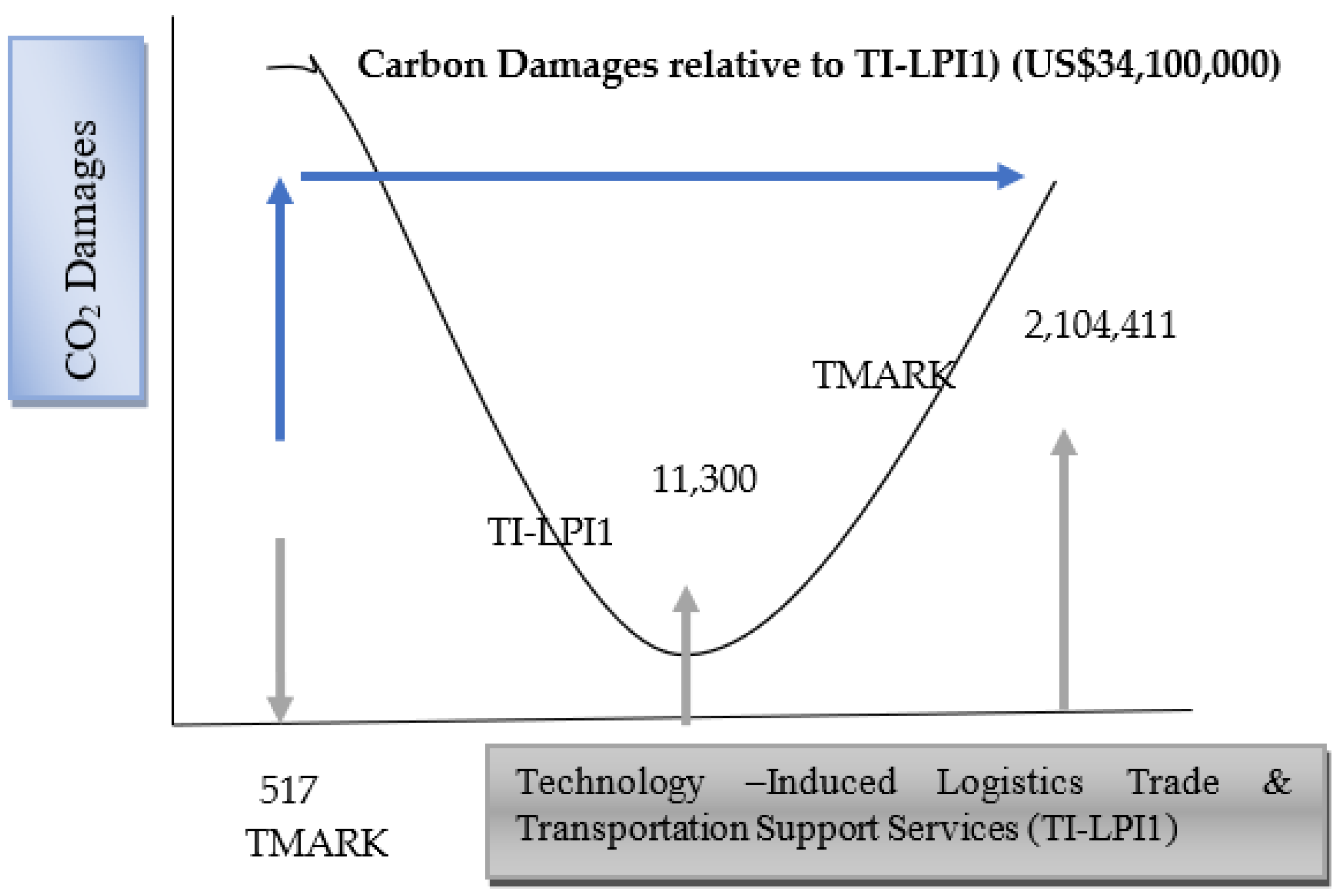
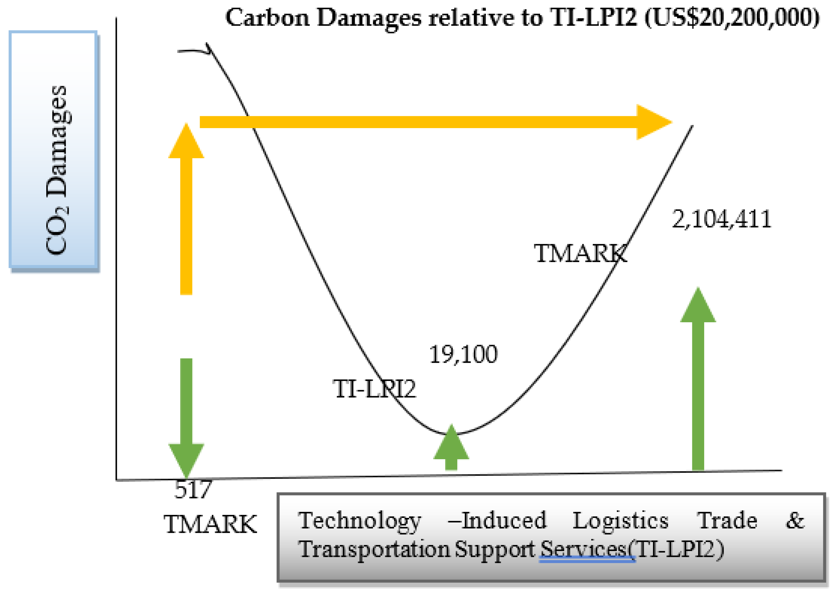
| Variables | Maximum | Minimum | Range | Cost of Carbon Emissions = Maximum value of Carbon Damages in US$/Turning Point | GDPPC | LPI1 × PATENTS | LPI2 × PATENTS | LPI1 × TMARK | LPI1 × TMARK |
| CDAM | 385,000,000,000 | 14,143,239 | 3.84,985,856,761 | US$15,000,000 | US$13,800,000 | US$6,100,000 | US$34,100,000 | US$20,200,000 | |
| GDPPC | 92,077.57 | 341.554 | 91,700 | ||||||
| LPI1 × PATENTS | 5,535,787 | 8.160 | 5,540,000 | ||||||
| LPI2 × PATENTS | 5,782,508 | 7.710 | 5,780,000 | ||||||
| LPI1 × TMARK | 7,618,117 | 956.450 | 7,620,000 | ||||||
| LPI1 × TMARK | 7,896,506 | 842.710 | 7,900,000 | ||||||
| Calculation from Prevention of Losses/Gains from Carbon Damages = (Cost of Carbon Damages in US$)–(Minimum Value of Carbon Damages in US$) OR (formula for calculating estimates in%) = [(Cost of Carbon Damages in US$)–(Minimum Value of Carbon Damages in US$)]/Minimum Value of CDAM in US$ | |||||||||
| GDPPC | US$856,761 (5.7%) | LPI1 × PATENTS | US$−343,239 (−2.4%) | LPI2 × PATENTS | US$−8,043,239 (−56.9%) | LPI1 × TMARK | US$19,956,761 (141.1%) | LPI2 × TMARK | US$6,056,761 (42.8%) |
| Panel–A: VAR Granger Causality | ||||||||||
| GDPPC→CDAM | χ2 value = 6.553 ** | PATENTS→CDAM | χ2 value = 439.515 * | PATENTS→CDAM | χ2 value = 439.515 * | |||||
| IND→GDPPC | χ2 value = 26.595 * | PATENTS→GDPPC | χ2 value = 5.377 *** | IND→IFS | χ2 value = 16.856 * | |||||
| GDPPC→LPI1 | χ2 value = 25.204 * | IND→LPI1 | χ2 value = 10.293 * | MHTECH→LPI1 | χ2 value = 16.211 * | |||||
| GDPPC→LPI2 | χ2 value = 47.457 * | MHTECH→LPI2 | χ2 value = 13.367 * | CDAM→PATENTS | χ2 value = 4.799 *** | |||||
| GDPPC→PATENTS | χ2 value = 8.309 ** | MHTECH→PATENTS | χ2 value = 5.162 *** | CDAM→TMARK | χ2 value = 99.932 * | |||||
| Panel–B: IRF Estimates Response of CDAM | ||||||||||
| Period | CDAM | GDPPC | IFS | IND | LPI1 | LPI2 | MHTECH | PATENTS | TMARK | |
| 1 | 979,000,000 | 0 | 0 | 0 | 0 | 0 | 0 | 0 | 0 | |
| 2 | 815,000,000 | 31,133,902 | 11,414,440 | −34,231,552 | 10,391,307 | 28,750,300 | 17,798,929 | 715,000,000 | 27,489,591 | |
| 3 | 836,000,000 | 44,423,031 | 9,741,106 | −37,524,336 | 17,275,727 | 39,453,430 | 28,485,206 | 538,000,000 | 174,000,000 | |
| 4 | 862,000,000 | 48,403,079 | 23,148,686 | −31,303,487 | 8,481,938 | 34,298,675 | 35,145,794 | 616,000,000 | 282,000,000 | |
| 5 | 885,000,000 | 47,191,581 | 28,977,373 | −25,077,303 | 11,590,938 | 36,444,242 | 45,351,963 | 659,000,000 | 390,000,000 | |
| 6 | 917,000,000 | 44,041,917 | 36,270,966 | −20,306,564 | 18,246,204 | 42,015,507 | 56,713,288 | 697,000,000 | 491,000,000 | |
| 7 | 955,000,000 | 40,016,487 | 42,266,737 | −16,354,633 | 28,334,800 | 50,099,640 | 69,736,073 | 734,000,000 | 584,000,000 | |
| 8 | 1,000,000,000 | 35,720,069 | 47,780,292 | −13,181,637 | 41,253,264 | 59,430,201 | 84,414,359 | 765,000,000 | 668,000,000 | |
| 9 | 1,050,000,000 | 31,352,273 | 52,662,917 | −10,519,072 | 56,344,268 | 69,242,784 | 101,000,000 | 793,000,000 | 743,000,000 | |
| 10 | 1,110,000,000 | 26,993,592 | 57,018,365 | −8,260,685 | 73,074,458 | 79,240,611 | 119,000,000 | 817,000,000 | 810,000,000 | |
| Panel–C: VDA Estimates of CDAM | ||||||||||
| Period | S.E. | CDAM | GDPPC | IFS | IND | LPI1 | LPI2 | MHTECH | PATENTS | TMARK |
| 1 | 979,000,000 | 100 | 0 | 0 | 0 | 0 | 0 | 0 | 0 | 0 |
| 2 | 1,460,000,000 | 75.85212 | 0.045348 | 0.006095 | 0.054821 | 0.005052 | 0.038670 | 0.014821 | 23.94772 | 0.035353 |
| 3 | 1,780,000,000 | 73.37281 | 0.093066 | 0.007121 | 0.081591 | 0.012854 | 0.075369 | 0.035681 | 25.33708 | 0.984421 |
| 4 | 2,090,000,000 | 70.08976 | 0.120948 | 0.017415 | 0.081457 | 0.010946 | 0.081452 | 0.054082 | 27.01669 | 2.527242 |
| 5 | 2,400,000,000 | 66.92227 | 0.130726 | 0.027854 | 0.072886 | 0.010662 | 0.085051 | 0.076916 | 28.11067 | 4.562959 |
| 6 | 2,710,000,000 | 63.99801 | 0.129068 | 0.039821 | 0.062825 | 0.012913 | 0.090845 | 0.104276 | 28.69388 | 6.868357 |
| 7 | 3,020,000,000 | 61.35512 | 0.121113 | 0.051528 | 0.053343 | 0.019158 | 0.100398 | 0.136958 | 28.92033 | 9.242052 |
| 8 | 3,340,000,000 | 59.06324 | 0.110328 | 0.062510 | 0.045119 | 0.030874 | 0.113598 | 0.175614 | 28.85943 | 11.53928 |
| 9 | 3,670,000,000 | 57.15358 | 0.098716 | 0.072366 | 0.038210 | 0.049126 | 0.129689 | 0.220861 | 28.57829 | 13.65917 |
| 10 | 4,010,000,000 | 55.63420 | 0.087370 | 0.080955 | 0.032488 | 0.074451 | 0.147898 | 0.273312 | 28.12958 | 15.53975 |
© 2020 by the authors. Licensee MDPI, Basel, Switzerland. This article is an open access article distributed under the terms and conditions of the Creative Commons Attribution (CC BY) license (http://creativecommons.org/licenses/by/4.0/).
Share and Cite
Anser, M.K.; Khan, M.A.; Awan, U.; Batool, R.; Zaman, K.; Imran, M.; Sasmoko; Indrianti, Y.; Khan, A.; Bakar, Z.A. The Role of Technological Innovation in a Dynamic Model of the Environmental Supply Chain Curve: Evidence from a Panel of 102 Countries. Processes 2020, 8, 1033. https://doi.org/10.3390/pr8091033
Anser MK, Khan MA, Awan U, Batool R, Zaman K, Imran M, Sasmoko, Indrianti Y, Khan A, Bakar ZA. The Role of Technological Innovation in a Dynamic Model of the Environmental Supply Chain Curve: Evidence from a Panel of 102 Countries. Processes. 2020; 8(9):1033. https://doi.org/10.3390/pr8091033
Chicago/Turabian StyleAnser, Muhammad Khalid, Muhammad Azhar Khan, Usama Awan, Rubeena Batool, Khalid Zaman, Muhammad Imran, Sasmoko, Yasinta Indrianti, Aqeel Khan, and Zainudin Abu Bakar. 2020. "The Role of Technological Innovation in a Dynamic Model of the Environmental Supply Chain Curve: Evidence from a Panel of 102 Countries" Processes 8, no. 9: 1033. https://doi.org/10.3390/pr8091033
APA StyleAnser, M. K., Khan, M. A., Awan, U., Batool, R., Zaman, K., Imran, M., Sasmoko, Indrianti, Y., Khan, A., & Bakar, Z. A. (2020). The Role of Technological Innovation in a Dynamic Model of the Environmental Supply Chain Curve: Evidence from a Panel of 102 Countries. Processes, 8(9), 1033. https://doi.org/10.3390/pr8091033