Decoupling Adaptive Smith Prediction Model of Flatness Closed-Loop Control and Its Application

Abstract

Flatness control system is characterized by multi-parameters, strong coupling, pure time delay, which complicate the establishment of an accurate mathematical model. Therefore, a control scheme that combines dynamic decoupling, PI (Proportion and Integral) control and adaptive Smith predictive compensation is proposed. To this end, a dynamic matrix is used to decouple the control system. A multivariable coupled pure time-delay system is transformed into several independent generalized single-loop pure time-delay systems. Then, a PI-adaptive Smith predictive controller is constructed for the decoupled generalized single-loop pure time-delay system. Simulations show that the scheme has a simple and feasible structure, and good control performance. When the mathematical model of the control system is inaccurate, the control performance of adaptive Smith control method is evidently better than that of the ordinary Smith control method. The model is successfully applied to the cold rolling production site through LabVIEW, and the control accuracy is within 5I. This study reveals a new solution to the problem of coupled pure time-delay in flatness control system.

1. Introduction

Cold rolling strip is characterized by high speed (rolling speed), heavy load, large width-thickness ratio, multi-parameters etc. It requires high dimensional accuracy (micron level) and short measurement and control period (millisecond level). In recent years, with the development of science and technology, some industries, such as automobiles, household appliances, precision instruments, aerospace equipment, etc., have higher and higher requirements on the quality of strip flatness. It is urgent to eliminate the strip flatness defects as much as possible [1]. The flatness control technology of cold rolling strip has a complex principle, numerous influencing factors and a strong technical comprehensiveness. It is involved in different fields, such as mechanical, material, instrument, control, electronics, information and computer, among others. It has also been a trending but complex research topic locally and abroad for decades [2,3,4,5,6,7,8]. Firstly, available flatness actuators, and the components that characterize flatness, are numerous; moreover, each adjustment actuator affects each flatness component, thereby making flatness control a multi-input and multi-output (MIMO) coupling control system [9]. Secondly, there is a certain distance between the position of the shapemeter and the roll gap. A period is spent for the shapemeter to measure the flatness after rolling, thereby making flatness control a typical pure time-delay control system. Thirdly, the open-loop gain matrix (influence matrix) calculated by the flatness control deformation mechanism model according to the set parameters deviates from the actual open-loop gain matrix because the actual rolling parameters fluctuate at any time [10]. Therefore, an accurate flatness control model is difficult to obtain.

In conclusion, the flatness control system is multi-parameter and has strong coupling and pure time-delay. As a result, the control model is difficult to establish timely and accurately, thereby increasing the instability and design difficulty of the system. For this reason, Wang et al., [11] proposed the Smith predictive control method, Ma [12], proposed the Dahlin–Smith predictive control algorithm and Liu et al., [13] proposed the dynamic variable gain control algorithm. Their studies were all based on the multi-point flatness control method, which has a large calculation amount and low calculation efficiency [14]. Furthermore, the control effect is poor when the model mismatches. Li Bo et al. [15] proposed a predictive control method, and Zhang et al., [16] proposed the Smith predictive control method. Their studies were based on the component flatness control method, which has a small calculation amount and high calculation efficiency. However, they all believed that an actuator only affects one flatness component, thereby neglecting the coupling effect of each flatness control loop. Moreover, the control effect is poor when the model is mismatched.

Following the above analysis, this study presents a decoupling adaptive Smith predictive control algorithm based on component flatness control. This algorithm handles the coupling and pure time-delay of the loop respectively, and simplifies the design of the control system. Initially, a multivariable coupled pure time-delay system is decoupled into several generalized single variable pure time-delay systems by using the dynamic decoupling matrix. Then, for the generalized single-loop pure time-delay system, an adaptive Smith predictor is designed to solve the problem of pure time-delay, and improve the control performance when the model is mismatched [17]. In this control system, the transverse multi-point flatness is recognized as several characteristic components by pattern recognition [18], and the overall flatness is controlled by controlling the characteristic components. Compared with the multi-point flatness control system, the calculation amount is greatly reduced. Based on the theory of MIMO, the essence of the flatness control system is revealed. The whole process decoupling of the control system is realized by using the diagonal matrix decoupling method. The overshoot and adjustment time of the system are reduced by using the adaptive Smith method. Compared with other components flatness control system, the control process is more stable and faster.

2. Flatness Decoupling Control System

2.1. Principle of Flatness Control

The position of intermediate roll shifting (IRS) of a 1420mm UCM (universal crown control mill) six-high cold rolling mill will be set and kept unchanged according to the rolling process before rolling, which is called set value control. Therefore, there are only three kinds of on-line adjustment means, roll tilting (RT), work roll bending (WRB) and intermediate roll bending (IRB). Following rolling deformation theory and the engineering practice, RT controls primary flatness mainly, whereas WRB and IRB control quadratic and quartic flatness mainly. Figure 1 shows the principle of flatness control, in which, σ = {σ₁, σ₂,…,σ_m} is a vector of the flatness of each section along the strip width direction measured by the shapemeter, and m is the number of measurement sections, where σ_m is the measured flatness value of the m-th measurement section. After flatness pattern recognition the measured flatness component coefficient vector A = {a₁, a₂, a₄} can be obtained, where a₁, a₂ and a₄, represent the measured primary, quadratic and quartic flatness component coefficients, respectively. A^T = {$a_1^T$, $a_2^T$, $a_4^T$} is the target flatness component coefficient vector, $a_1^T$, $a_2^T$ and $a_4^T$ represent the primary, quadratic and quartic target flatness component coefficient respectively. E = A^T – A = {e₁, e₂, e₄} is the vector of flatness deviation component coefficient, where e₁, e₂ and e₄ represent the primary, quadratic and quartic flatness deviation coefficient components respectively. ΔU = {Δu₁, Δu₂, Δu₄} is the regulator vector of a given flatness adjustment parameter, where Δu₁, Δu₂ and Δu₄ are the given RT displacement adjustment, WRB and IRB force adjustment respectively. ΔU^* = {Δ$u_1^{*}$, Δ$u_2^{*}$, Δ$u_4^{*}$} is the actual output flatness adjustment parameter adjustment vector, Δ$u_1^{*}$, Δ$u_2^{*}$ and Δ$u_4^{*}$ are the actual adjustment of RT displacement adjustment, WRB and IRB force adjustment respectively. In each control cycle, the flatness control system makes the target flatness A^T minus the measured flatness A initially obtain the flatness deviation E. Then, it calculates the adjustment amount ΔU according to the flatness deviation E and sends it to the hydraulic system. Lastly, the hydraulic system of each actuator outputs the actual adjustment amount ΔU^* to the roll system according to its dynamic response. Meanwhile, the flatness of the roll gap is changed by changing its shape. The flatness after rolling reaches the shapemeter after τ = l/v time in which l (m) is the distance between the roll gap and the shapemeter, and v (m/s) is the rolling speed.

2.2. Flatness Open-Loop Control Model

The flatness control system of the 1420 mm UCM six-roll cold rolling mill shown in Figure 1 is a three-input-three-output MIMO coupling pure time-delay control system. In accordance with the flatness control principle in Figure 1, the flatness open-loop control system which is shown in Figure 2 is constructed; in such system, G_TM(s) = G_T(s)G_M(s), G_WM(s) = G_W(s)G_M(s), G_IM(s) = G_I(s)G_M(s), where G_T(s), G_W(s), G_I(s) and G_M(s) are the transfer functions of RT, WRB, IRB and shapemeter, respectively. Here, Δa₁, Δa₂ and Δa₄ are the changes of the flatness coefficients of primary, quadratic and quartic flatness, respectively; meanwhile, $a_1^0$, $a_2^0$ and $a_4^0$ are the initial measured (last time) primary, quadratic and quartic flatness coefficients respectively. Element c_ij is the open-loop gain of the flatness control system, whose physical meaning is the influence coefficient of the j-th adjustment means on the i-th flatness component coefficient. The open-loop gain matrix of the flatness control is constituted by flatness component coefficient, which is called the flatness adjustment influence matrix C [19].

$$C=\left[\begin{array}{ccc}{c}_{11}& c_{12}& c_{13}\\ c_{21}& c_{22}& c_{23}\\ c_{41}& c_{42}& c_{43}\end{array}\right]c_{ij}=\Delta a_i/\Delta u_j^{*}$$

(1)

Equation (1), Δa_i is the change of the i-th flatness component and Δ$u_j^{*}$ is the change of the j-th actuator. The transfer functions of hydraulic system of RT, WRB and IRB of the cold rolling mill and the shapemeter are shown in Equation (2), which can be approximated to a first-order model [20].

$$G_T(s)=\frac{1}{T_{T}s+1}, G_W(s)=\frac{1}{T_{W}s+1}, G_I(s)=\frac{1}{T_{I}s+1}, G_M(s)=\frac{1}{T_{M}s+1}$$

(2)

Equation (2), s is the variable after Laplace transformation (differential operator). T_T, T_W, T_I and T_M are the time constants of the RT, WRB, and IRB system and the shapemeter, respectively. After the transfer function of each link and the influence matrix of flatness adjustment are known, the transfer function matrix G(s) of flatness control is obtained as follows. Equation (3), e^-τs indicates that the system has a time-delay of τ seconds.

$$G(s)=\left[\begin{array}{ccc}{c}_{11}{G}_{TM}{e}^{-\tau s}& c_{12}{G}_{WM}{e}^{-\tau s}& c_{14}{G}_{IM}{e}^{-\tau s}\\ c_{21}{G}_{TM}{e}^{-\tau s}& c_{22}{G}_{WM}{e}^{-\tau s}& c_{24}{G}_{IM}{e}^{-\tau s}\\ c_{41}{G}_{TM}{e}^{-\tau s}& c_{42}{G}_{WM}{e}^{-\tau s}& c_{44}{G}_{IM}{e}^{-\tau s}\end{array}\right]$$

(3)

2.3. Flatness Closed-Loop Decoupling Control Model

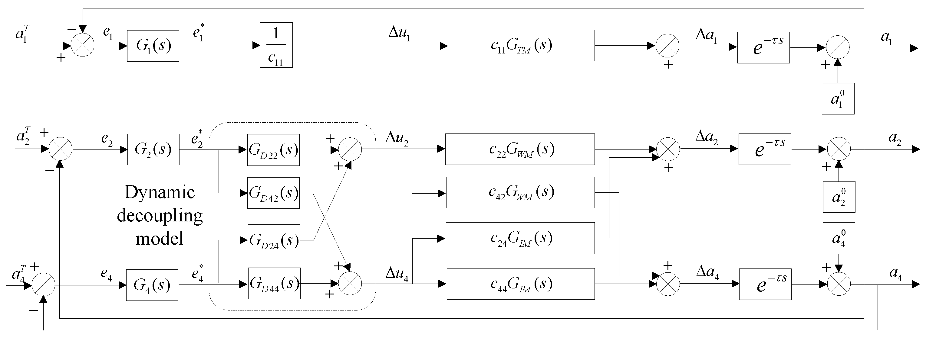
The pure time-delay time of each flatness component control loop is the same. Hence, the coupling and the time-delay parts of the strip control system can be dealt, respectively. For the coupling part in Figure 2, the coupling system can be transformed into three generalized single-loop control systems by decoupling. In this study, the closed-loop control strategy of independent control primary flatness, decoupling control quadratic and quartic flatness proposed by the author in another study is adopted [21]. The slight influence of RT on quadratic and quartic flatness and the slight influence of WRB and IRB on primary flatness are ignored. Figure 3 shows the flatness closed-loop decoupling control system. The dotted lines in Figure 3 is a dynamic decoupling model. G_D22(s), G_D42(s), G_D24(s) and G_D44(s) are the four elements of the dynamic decoupling matrix G_D(s). G₁(s), G₂(s) and G₄(s) are primary, quadratic and quartic flatness PI controllers, respectively. E^* = {$e_1^{*}$, $e_2^{*}$, $e_4^{*}$} is the coefficient vector of flatness deviation component output by PI controllers, in which $e_1^{*}$, $e_2^{*}$ and $e_4^{*}$ are the primary, quadratic and quartic flatness deviation components output by PI controllers, respectively. In accordance with diagonal matrix decoupling theory [22], the control system will be decoupled completely when the dynamic decoupling matrix satisfies Equation (4), and the Equation (5) is obtained, which is called dynamic decoupling matrix.

$$\left[\begin{array}{cc}{c}_{22}{G}_{WM}(s)& c_{24}{G}_{IM}(s)\\ c_{42}{G}_{WM}(s)& c_{44}{G}_{IM}(s)\end{array}\right]\times \left[\begin{array}{cc}{G}_{D22}(s)& G_{D24}(s)\\ G_{D42}(s)& G_{D44}(s)\end{array}\right]=\left[\begin{array}{cc}{G}_{WM}(s)& 0\\ 0& G_{IM}(s)\end{array}\right]$$

(4)

$$G_D(s)=\frac{1}{c_{22}{c}_{44}-c_{24}{c}_{42}}\left[\begin{array}{cc}{c}_{44}& -c_{24}{G}_{IM}(s)/G_{WM}(s)\\ -c_{42}{G}_{WM}(s)/G_{IM}(s)& c_{22}\end{array}\right]$$

(5)

3. Flatness Decoupling Adaptive Smith Predictive Control

3.1. Primary Flatness Adaptive Smith Predictive Control

Decoupling control solves the coupling problem of the flatness control system, but does not solve the pure time-delay problem. The decoupled flatness control system can be regarded as three independent loops, and the predictive controller can be designed by solving single-loop pure time-delay; in this manner, the controller design is simplified and the practicability of the controller is enhanced [23,24]. Smith predictive control is an effective solution to the problem of single-loop pure time-delay. However, it depends on an accurate control object model to obtain good control effect [25,26]. However, in the general industrial process, the control object often contains uncertainties. As a result, the predictive model is difficult to match with the control object completely. Therefore, the desired control effect is difficult to achieve when the traditional Smith predictive control algorithm used [27]. In view of this deficiency of Smith predictive control, an adaptive Smith predictive control algorithm is proposed. By adjusting the parameters of the cascade controller adaptively, the output of the controller can be adjusted in real time to reduce the overshoot and adjustment time caused by model mismatch and enhance the stability of the system. Each control loop can be described by a first-order plus pure time-delay model because T_M is more than one order of magnitude smaller than T_T, T_W and T_I. In other words, G_TM(s) ≈ G_T(s), G_WM(s) ≈ G_W(s) and G_IM(s) ≈ G_I(s) as shown in Figure 3. By taking the primary flatness control loop as an example, and ignoring the slight influence of WRB and IRB on primary flatness, the cascade controller adopts proportional control K₁(t) to obtain a PI-adaptive Smith predictive control system of primary flatness as shown in Figure 4, where, $K_1^{*}$, $G_{\mathit{TM}}^{*}$(s) and τ^* are the open-loop gain coefficient, dynamic response and delay time of the primary flatness Smith predictor, respectively. Δ$a_1^{*}$ is the primary flatness change output of the Smith predictor, and e_y1 is the deviation between the actual and predicted outputs of the primary flatness control loop.

Let $G_{\mathit{TM}}^{*}$(s) = 1/($T_T^{*}$ + 1), where $T_T^{*}$ is the time constant of Smith predictor, the following can be inferred from Figure 4. Δ$a_1^{\prime }$(t) and Δ$a_1^{*\prime }$(t) are the derivatives of Δa₁ (t) and Δ$a_1^{*}$(t) with respect to t, respectively.

$$\Delta a_1^{\prime }(t)=-\frac{1}{T_T}\Delta a_1(t)+\frac{K_1(t)}{T_T}{e}_1^{*}(t)$$

(6)

$$\Delta a_1^{*\prime }(t)=-\frac{1}{T_T^{*}}\Delta a_1^{*}(t)+\frac{K_1^{*}}{T_T^{*}}{e}_1^{*}(t)$$

(7)

$$e_{y1}(t)=\Delta a_1(t)e^{-\tau t}-\Delta a_1^{*}(t)e^{-{\tau }^{*}t}$$

(8)

Given $G_{TM}^{*}$(s) = 1/($T_T^{*}$ + 1) and $T_T^{*}$ = T_T, we can rewrite Equation (8) to Equation (9) because e^-τs only shifts Δa₁(t) and Δ$a_1^{*}$(t) on the time axis by a time τ, which can be calculated, so the time-delay can be ignored [28]. Transforming Equation (8) to time domain and ignoring time-delay, it can be written as Equation (9).

$$e_{y1}(t)=\Delta a_1(t)-\Delta a_1^{*}(t)$$

(9)

Taking the derivative of Equation (9), Equation (10) can be obtained.

$$e_{y1}^{\prime }(t)=-\frac{1}{T_T}{e}_{y1}(t)+\frac{1}{T_T}[K_1(t)-K_1^{*}]e_1^{*}(t)$$

(10)

Given Ω as a two-dimensional space containing variables e_y1(t) and K₁(t) − $K_1^{*}$, and ε^T = {e_y1(t), (K₁(t) − $K_1^{*}$)} as a vector of space Ω, we choose Equation (11) as a Lyapunov-function [29].

$$V(\epsilon )=\frac{1}{2}\left\{T_T{e}_{y1}^2(t)+\frac{1}{{\lambda }_1}{[K_1(t)-K_1^{*}]}^2\right\}$$

(11)

Equation (11), λ₁ is a constant greater than zero, and T_T > 0 holds for all V(ε) > 0. Taking the derivative of Equation (11), Equation (12) can be obtained.

$$V^{\prime }(\epsilon )=T_T{e}_{y1}(t)e_{y1}^{\prime }(t)+\frac{1}{{\lambda }_1}[K_1(t)-K_1^{*}]K_1^{\prime }(t)$$

(12)

By bring Equation (10) in Equation (12) and sorting out, Equation (13) can be obtained.

$$V^{\prime }(\epsilon )=-e_{y1}^2(t)+[K_1(t)-K_1^{*}][\frac{1}{{\lambda }_1}{K}^{\prime }(t)+e_{y1}(t)e_1^{*}(t)]$$

(13)

Given $K_1^{\prime }$(t) = −λ₁e_y1(t)$e_1^{*}$(t), Equation (14) can be obtained.

$$K_1(t)=-{\lambda }_1\int e_{y1}(t)e_1^{*}(t)dt+K_1(0)$$

(14)

$$V^{\prime }(\epsilon )=-e_{y1}^2(t)\le 0$$

(15)

Equation (14), K₁(0) is the initial value of K₁(t). Following Lyapunov’s asymptotic stability theorem [30], Equation (10) is asymptotically stable, when V′(ε) ≤ 0. Equation (14) is the adaptive equation. To speed up the adjustment speed and improve the performance of the adaptive algorithm K₁(t), an adaptive algorithm for the primary flatness is obtained as Equation (16) by adding ${-\lambda }_1^{*}$e_y1(t)$e_1^{*}$(t) (${\lambda }_1^{*}$ is a constant greater than zero) to the adaptive equation [31,32].

$$K_1(t)=-{\lambda }_1\int e_{y1}(t)e_1^{*}(t)dt-{\lambda }_1^{*}{e}_{y1}(t)e_1^{*}(t)+K_1(0)$$

(16)

3.2. Quadratic and Quartic Flatness Decoupling Adaptive Smith Predictive Control

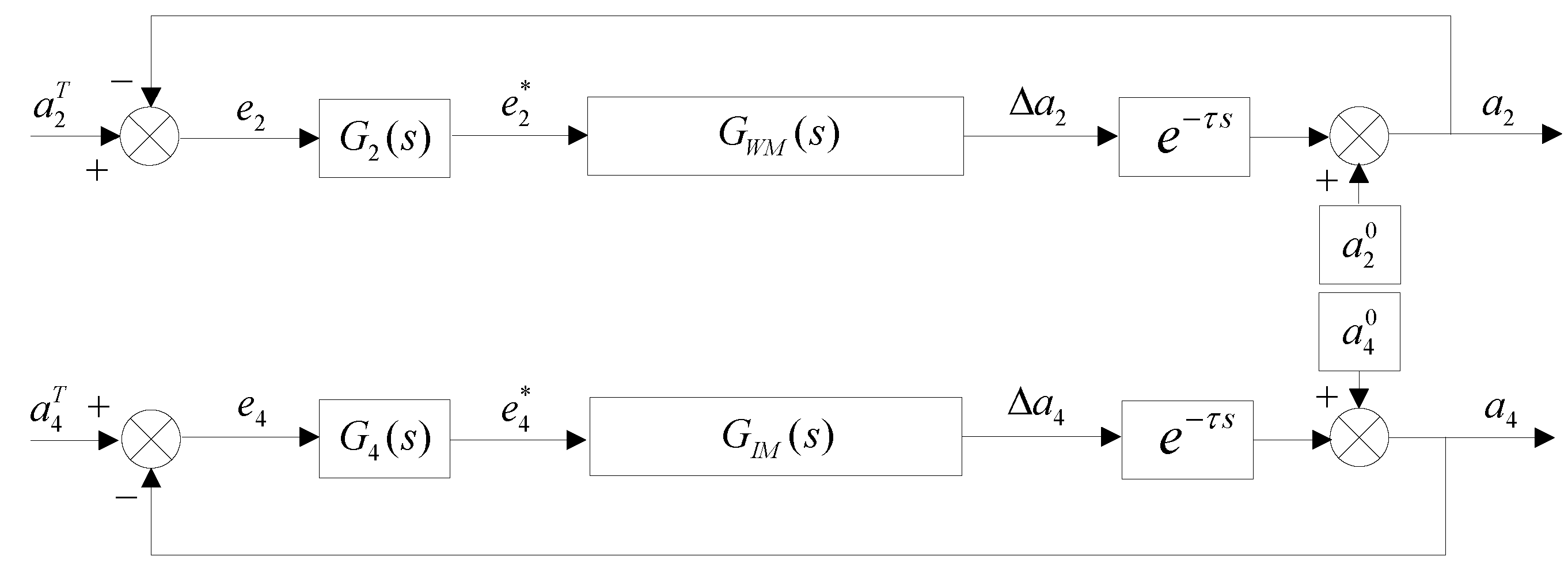
The decoupled quadratic and quartic flatness control loops are two independent and uncoupled single-loops as shown in Figure 5. Each adaptive Smith predictive control system can be designed on the basis of single-loop. Ignoring the slight influence of RT on the quadratic and quartic flatness, and the cascade controllers adopt proportional control, the quadratic and quartic flatness decoupling PI-adaptive Smith predictive control system shown in Figure 6 is obtained. K₂(t) and K₄(t) are the quadratic and quartic flatness cascade proportional controllers, $K_2^{*}$ and $K_4^{*}$ are the open-loop gain coefficients of the quadratic and quartic flatness Smith predictors, $G_{WM}^{*}$(s) and $G_{IM}^{*}$(s) are the dynamic responses of the quadratic and quartic flatness Smith predictors, Δ$a_2^{*}$ and Δ$a_4^{*}$ are the quadratic and quartic flatness changes of the Smith predictors, and e_y2 and e_y4 are the deviation between the actual and predicted outputs of the quadratic and quartic flatness control loops respectively. Referring to the adaptive algorithm of primary flatness control, the adaptive algorithm of quadratic and quartic flatness control loops is obtained as shown in Equation (17) and Equation (18), respectively, in which K₂(0) and K₄(0) are the initial values of K₂(t) and K₄(t), respectively, and λ₂, ${\lambda }_2^{*}$, λ₄ and ${\lambda }_4^{*}$ are four constants greater than zero.

$$K_2(t)=-{\lambda }_2\int e_{y2}(t)e_2^{*}(t)dt-{\lambda }_2^{*}{e}_{y2}(t)e_2^{*}(t)+K_2(0)$$

(17)

$$K_4(t)=-{\lambda }_4\int e_{y4}(t)e_4^{*}(t)dt-{\lambda }_4^{*}{e}_{y4}(t)e_4^{*}(t)+K_4(0)$$

(18)

4. Simulation Comparison and Industrial Application

4.1. Simulation Comparison

T_T, T_W, T_I and T_M are 0.05 s, 0.15 s, 0.25 s and 0.003 s of a 1420 mm UCM six-roll cold rolling mill in a factory respectively. The normal rolling speed of the mill is between 5.0 and 13.3 m/s (according to field rolling process), and the distance between the shapemeter and the roll gap is 2.0 m (field measurement). Therefore, the delay time is between 0.15 and 0.4 s. The normal rolling speed of the strip with a width of 1230 mm is 10 m/s, i.e., delay time τ = 0.2 main rolling parameters and the flatness adjustment influence matrix (calculating matrix) calculated from the flatness control deformation mechanism model are shown in

Table 1. Main rolling parameters and calculating matrix.

Strip Width /mm	Rolling Force /10kN	Entry Thickness /mm	Exit Thickness /mm	Front Force /kN	Post Tension /kN	IRS /mm	Calculating Matrix C0
1230	864	1.04	0.79	107	80	115	$\begin{array}{ccc}-0.1829& -0.0001& 0.0002\\ 0.0003& -0.4084& 0.0398\\ 0.0005& 0.3079& 0.0373\end{array}$

[33]. The simulation systems of flatness control Simulink based on decoupling PI, decoupling PI-Smith and decoupling PI-adaptive Smith are built, respectively. Figure 5 shows that when the model matches perfectly, the open-loop gain coefficient of the generalized quadratic and quartic flatness control loops after decoupling is 1. Hence, the initial value of the cascade controller of the quadratic and quartic flatness control loops and the open-loop gain of Smith predictor are all 1, i.e., K₂(0) = 1, K₄(0) = 1, $K_2^{*}$ = 1 and $K_4^{*}$ = 1, similarly K₁(0) = 1, $K_1^{*}$ = 1. The parameters of each loop controller and the adaptive parameters are selected as shown in

Table 2. Main parameters of control system.

KP1	KI1	λ1	λ1*	KP2	KI2	λ2	λ2*	KP4	KI4	λ4	λ4*
0.2	0.033	0.01	0.5	0.6	0.107	0.03	0.45	0.5	0.167	0.02	0.40

, in which K_P1, K_I1, K_P2, K_I2, K_P4 and K_I4 are the proportional and integral coefficients of the primary, quadratic and quartic flatness PI controllers, respectively. Taking the primary flatness control loop as an example, its PI controller equation is shown in Equation (19) [34].

$$u_t=K_{p}e(t)+K_I\int e(t)dt$$

(19)

In accordance with Equation (3), the transfer function matrix of the flatness control system is composed of three parts: influence matrix, dynamic response and time-delay. RT, WRB and IRB are the inner rings of flatness control. Their time constants, i.e., their dynamic response is determined. The delay time is τ = l/v, where l is fixed, and v is measured in real time, so the delay time is determined. Therefore, the major factor affecting the transfer function matrix is the influence matrix. The influence matrix for control is usually calculated from the flatness control deformation mechanism model according to the set (specific) parameters, which is called calculating matrix. The actual rolling parameters fluctuate at any time, thereby result in a large deviation between the calculating matrix and the actual matrix, which can be calculated in accordance with the measured data of the rolling process and changes at any time. In summary, only the influence matrix is uncertain in the flatness control system model. Hence, in this study, only the matching and mismatching control performance comparison between the calculating matrix of the decoupling part and the actual matrix of the coupling part are discussed.

Assuming the initial flatness is $a_1^0$ = 0, $a_2^0$ = 0 and $a_4^0$ = 0, let $a_1^T$ = 1, $a_2^T$ = 1 and $a_4^T$ = 1, and the various situations of actual matrix and calculating matrix of rolling mill are simulated and compared. Three representative cases are presented in

Table 3. Actual matrix.

C0	C1	C2
$\begin{array}{ccc}-0.1829& -0.0001& 0.0002\\ 0.0003& -0.4084& 0.0398\\ 0.0005& 0.3079& 0.0373\end{array}$	$\begin{array}{ccc}-0.2560& -0.0001& 0.0003\\ 0.0004& -0.5718& 0.0557\\ 0.0007& 0.4310& 0.0522\end{array}$	$\begin{array}{ccc}-0.1097& -0.0001& 0.0001\\ 0.0002& -0.2450& 0.0239\\ 0.0003& 0.1847& 0.0224\end{array}$

and Figure 7. The interpretations of the curves in Figure 7 are shown in

Table 4. The meanings of the curves in Figure 7.

Curve label	A	B	C	D	E	F
Calculating matrix	C0	C0	C0	C0	C0	C0
Actual matrix	C0	C0	C1	C1	C2	C2
Control method	PI	PI-Smith	PI-Smith	PI-adaptive Smith	PI-Smith	PI-adaptive Smith

.

(1) From the comparison of Curves A and B, when the model matches perfectly, after adding Smith predictive control, the flatness components are not overshoot and the adjustment time is greatly shortened. Hence the control strategy of decoupling first and then Smith predictive control is effective.

(2) From the comparison of Curves C and D, when the absolute value of each element of the actual matrix is larger than that of the calculating matrix, PI-Smith predictive control produces large overshoots for each flatness component. After using PI-adaptive Smith predictive control, the overshoots of the primary and quadratic flatness are evidently reduced, the quartic flatness is no overshoot.

(3) From the comparison of Curves E and F, when the absolute value of each element in the actual matrix is smaller than that of the calculating matrix, and the adjustment time of each flatness component is long using PI-Smith predictive control, whereas that of PI-adaptive Smith predictive control is short.

In summary, the flatness control system using decoupled PI-adaptive Smith predictive control can greatly reduce overshoot caused by pure time-delay, shorten the adjustment time, and stabilize control process. Furthermore, the adaptive algorithm can improve the control quality of the system when the mathematical model is mismatched.

4.2. Industrial Application

The flatness control method proposed in this paper has been applied to a 1420 mm UCM six-high cold rolling mill. The control program is written with LabVIEW as the development environment, and its application process principle is shown in Figure 8. Ni OPC server is the bridge between LabVIEW and S7-400 to establish data connection, and plays the function of communication protocol conversion. The flatness control program first reads the parameters needed for flatness control in S7-400 through Ni OPC server, then reads the measured flatness of the flatness measuring host through the switch, calculates the flatness control amount and writes it into S7-400 through Ni OPC server, and finally, S7-400 gives the control adjustment amount to the corresponding actuator through its input and output (I/O) equipment. The variation range of RT is–150 µm ~ 150 µm, the variation range of WRB is −200kN ~ 500kN, the variation range of IRB is 0kN ~ 500kN, and the variation range of IRS is −200mm ~ 200mm. Take the strip of Table 1 as an example, control period is 50ms, the target flatness $a_1^T$ = 0, $a_2^T$ = 0 and $a_4^T$ = 0, the initial RT is 0μm, the initial WRB is 110 kN, the initial IRB is 120 kN, the actual change of flatness component coefficient, actuator adjustment amount, the overall flatness change process and the strip after rolling are shown in (a), (b), (c) and (d) of Figure 9, respectively. The flatness data is from the flatness control host (sampling period 50 ms), and the actual change of actuator adjustment parameters is from the factory PDA (sampling period 1ms).

It can be seen that the controlled primary, quadratic and quartic flatness coefficients do not overshoot and reach the target value in about 1.5 s. After control, the flatness of all transverse parts of the strip are within ±5I. The remaining flatness defects are high-order, whose shape is wave, which indirectly shows that RT, WRB and IRB can’t adjust the high-order flatness. In the process of adjustment, only the IRB produces overshoot of about 10%, and the RT and WRB do not produce overshoot. The overall flatness of the strip changes rapidly and stably, and the surface shape of the strip is good after rolling without obvious deformation. After a long time of industrial application, different specifications of strip only have different response of the actuator and flatness during the adjustment process, the adjustment time is mostly within 2.5 s, and the final flatness deviation is mostly within ± 5I, which shows that the decoupling strategy and control method proposed in this paper are effective. With the setting value of IRS is appropriate, the integral flatness deviation of strip can be eliminated by adjusting the primary, quadratic and quartic flatness components through roll RT, WRB and IRB, and the local flatness deviation cannot be eliminated.

5. Discussion

The flatness control system can control the overall flatness of strip by controlling the three characteristic components: primary, quadratic and quartic. Compared with the multi-point flatness control system in references 11–14, the design is simple, the control variables are fewer, and the calculation amount is small. When the control system model is mismatched, the adjustment time of the system is shorter, the flatness control process is more stable and the actuator will not produce large overshoot. Compared with the predictive control algorithm in reference 15, the process coupling of the system is considered in this paper. The dynamic term is added to the decoupling process to realize the whole process decoupling of the control system. Moreover, the influence of various actuators means that the flatness components is considered, so the design of the control system is more perfect and the operation more stable. Compared with the traditional Smith predictive control algorithm in reference 16, the adaptive Smith algorithm proposed in this paper is more suitable for industrial field, the flatness control effect is better, the overshoot of actuator is smaller, and the adjustment time is shorter. Because the control system is specially designed for a 1420 mm UCM reversible cold rolling mill, it is not equipped with subsection cooling system, the system cannot be combined with subsection cooling, and the flatness control accuracy remains at ± 5I, which cannot be further improved.

6. Conclusions

1. Through analysis the internal structure of the flatness control system, the control strategy of decoupling first and then compensating time-delay is proposed. A complex multi-loop coupled time-delay system is decoupled into simple multi-generalized single-loop time-delay systems. In this manner, the design difficulty of the control system is simplified.

2. To address solve the difficulty in accurately calculating the influence matrix of flatness adjustment and the poor effect of ordinary Smith predictive control method, this study proposes an adaptive Smith predictive control method. Adjusting the cascade controller coefficients in real time reduces the overshoot and adjustment time caused by model mismatch, improving the control quality.

3. The simulation results show that for the time-delay flatness control system Smith predictive control is effective when the model is matched. When the control model is mismatched, the adaptive Smith method is better than the ordinary Smith method.

4. The industrial application shows that the setting value of IRS is appropriate, the integral flatness deviation of strip can be controlled within ± 5I by adjusting the primary, quadratic and quartic flatness components, through roll RT, WRB and IRB, and the local flatness deviation cannot be eliminated.

References

1. Yang, L.P.; Yu, H.X.; Zhang, Y.S.; Liu, H.M. Shape Detection and Control System of Cold Rolling Strip Based on the Virtual Instrument and Its Industrial Application. J. Mech. Eng. 2018, 54, 1–7. [Google Scholar] [CrossRef]
2. Li, X.; Luan, F.; Wu, Y.A. Comparative Assessment of Six Machine Learning Models for Prediction of Bending Force in Hot Strip Rolling Process. Metals 2020, 10, 685. [Google Scholar] [CrossRef]
3. Pin, G.; Francesconi, V.; Cuzzola, F.A.; Parisini, T. Adaptive task-space metal strip-flatness control in cold multi-roll mill stands. J. Process Control 2013, 23, 108–119. [Google Scholar] [CrossRef]
4. Jin, X.; Li, C.S.; Wang, Y.; Li, X.G.; Xiang, Y.; Gu, T. Investigation and Optimization of Load Distribution for Tandem Cold Steel Strip Rolling Process. Metals 2020, 10, 677. [Google Scholar] [CrossRef]
5. Ogasahara, T.; Kitamura, T.; Aoe, S.I.; Tateno, J.I.; Asano, K. Dynamic Control of Flatness and Elongation of the Strip in a Skin Pass Mill. Tetsu Hagane 2019, 105, 512–521. [Google Scholar] [CrossRef]
6. Xie, H.B.; Li, L.J.; Liu, T.W.; Wang, E.R.; Liu, X.; Jiang, Z.Y. Three Dimensional Finite Element Simulation of Strip Shape and Flatness of High Strength Steel. Key Eng. Mater. 2019, 794, 232–245. [Google Scholar] [CrossRef]
7. Kozhevnikov, A.; Kozhevnikov, I.; Bolobanova, N. Dynamic model of cold strip rolling. Metalurgija 2018, 57, 99–102. [Google Scholar]
8. Ataka, M. Rolling Technology and Theory for the Last 100 Years: The Contribution of Theory to Innovation in Strip Rolling Technology. ISIJ Int. 2015, 55, 89–102. [Google Scholar] [CrossRef] [Green Version]
9. Liu, H.M.; He, H.T.; Shan, X.Y.; Jiang, G.B. Flatness Control Based on Dynamic Effective Matrix for Cold Strip Mills. J. Mech. Eng. 2009, 22, 41–75. [Google Scholar] [CrossRef]
10. Yang, L.P.; Yu, H.Y.; Wang, D.C.; Zhang, Z.; Jiang, Z.Y. Intelligent Shape Regulation Cooperative Model of Cold Rolling Strip and Its Application. Steel Res. Int. 2017, 88, 1600383. [Google Scholar] [CrossRef]
11. Wang, P.F.; Peng, Y.; Wang, D.C.; Sun, J.; Zhang, D.H.; Liu, H.M. Flatness Control Strategy Based on Delay Compensation for Cold Rolling Mill. Steel Res. Int. 2017, 88, 1600065. [Google Scholar]
12. Ma, L. Strategy of Flatness Control System Lag Compensation. Master’s Thesis, Yanshan University, Qinhuangdao, China, 2014. [Google Scholar]
13. Liu, J.W.; Jiang, D.P.; Wu, H.L.; Chen, R.J. Algorithm Research and Application of dynamic variable gain controller based on flatness control in cold mill. In Proceedings of the 8th Youth Academic Annual Meeting of China Metal Society, Beijing, China, 23–25 October 2013; pp. 1–6. [Google Scholar]
14. Wang, P.F.; Zhang, Z.J.; Sun, J.; Zhang, D.H.; Liu, H.M.; Gao, X.L. Flatness control of cold rolled strip based on relay optimization. Ironmak. Steelmak. 2016, 45, 166–175. [Google Scholar] [CrossRef]
15. Li, B.; Zhang, Q.D. Study on Flatness Predictive Control for CVC-4th Cold Mill. Metall. Equip. 2008, 4, 9–12. [Google Scholar]
16. Zhang, R.C.; Zheng, X. Automatic flatness control strategy with a Smith predictor for steel strip rolling. In Proceedings of the 2011 International Conference on Photonics, 3D-Imaging, and Visualization, Guangzhou, China, 30–31 October 2011; pp. 1–6. [Google Scholar]
17. Xing, Z.W.; Ding, B.J. Intelligent Control Method for Aircraft Deicing Fluid temperature Based on a New Adaptive Smith Predictor. Adv. Mater. Res. 2012, 424, 936–940. [Google Scholar] [CrossRef]
18. Song, M.M.; Wang, D.C.; Zhang, S.; Xu, Y.H.; Liu, H.M. Flatness pattern recognition based on recurrent neural network. Iron Steel 2018, 53, 56–62. [Google Scholar]
19. Yang, L.P.; Zhang, Z.; Wang, D.C.; Li, R.M.; Yu, H.X.; Zhang, Y.S. Mechanism-intelligent coordination shape control model of cold strip. Iron Steel 2017, 52, 52–57. [Google Scholar]
20. Zhu, Y.; Tang, S.; Wang, C.; Jiang, W.; Zhao, J.; Li, G. Absolute stability condition derivation for position closed-loop system in hydraulic automatic gauge control. Processes 2019, 7, 766. [Google Scholar] [CrossRef] [Green Version]
21. Song, M.M.; Liu, H.M.; Wang, D.C.; Xu, Y.H. Decoupling Strategy and Dynamic Decoupling Model of Flatness Control in Cold Rolling Strip. ISIJ Int. 2020, 60, 286–296. [Google Scholar] [CrossRef]
22. Wang, J.; Yan, W.; Shao, H. Performance improvement of VAV air conditioning control system through diagonal matrix decoupling and Lonworks technology. Energy Build. 2005, 37, 911–919. [Google Scholar] [CrossRef]
23. Chou, J.H.; Chang, J.F.; Lin, D.B.; Wu, T.L. Dual-band WLAN MIMO antenna with a decoupling element for full-metallic bottom cover tablet computer applications. Microw. Opt. Technol. Lett. 2018, 60, 1245–1251. [Google Scholar] [CrossRef]
24. Xu, S.; Hashimoto, S.; Jiang, W. Pole-Zero Cancellation Method for Multi Input Multi Output (MIMO) Temperature Control in Heating Process System. Processes 2019, 7, 497. [Google Scholar] [CrossRef] [Green Version]
25. Kaya, I. Improving performance using cascade control and a Smith predictor. ISA Trans. 2001, 40, 223–234. [Google Scholar] [CrossRef]
26. Wang, Y.Q.; Sun, F.; Liu, J.; Sun, M.H.; Xie, Y.H. Application of Smith Predictor Based on Single Neural Network in Cold Rolling Shape Control. Chin. J. Mech. Eng. 2009, 22, 282–286. [Google Scholar] [CrossRef]
27. Zhang, P.; Yuan, M.Z.; Wang, H. Self-adaptive Fuzzy-Smith Control for a Long Time-delay System. Comput. Simul. 2006, 23, 88–90. [Google Scholar]
28. Li, X.; Song, D.Q.; Yu, S.Y.; Gui, W.H. Feedback automatic gauge control system using model reference adaptive Smith predictor. Control Theory Appl. 2009, 26, 999–1003. [Google Scholar]
29. Gao, H.J.; Lam, J.; Chen, T.W.; Wang, C.H. Stability analysis of uncertain discrete-time systems with time-varying state delay: A parameter-dependent Lyapunov function approach. Asian J. Control 2010, 8, 433–440. [Google Scholar] [CrossRef]
30. Zheng, D.Z. Liner System Theory; Tsinghua University Press: Beijing, China, 1990; pp. 213–242. [Google Scholar]
31. Zhou, Y.; Song, D.D.; Nie, P.P.; Hao, H.M. Application of model reference adaptive control-improved Smith-predictor in temperature control of fermentation. J. Hebei Univ. Tech. 2011, 40, 5–9. [Google Scholar]
32. Song, Y.X.; Zhu, X.F. An Improved Adaptive Smith Predictor System. Meas. Control Tech. 2002, 8, 37–40. [Google Scholar]
33. Wang, D.C.; Liu, H.M. A Model Coupling Method for Shape Prediction. J. Iron Steel Res. Int. 2012, 19, 22–27. [Google Scholar] [CrossRef]
34. Rodríguez-Miranda, E.; Beschi, M.; Guzmán, J.L.; Berenguel, M.; Visioli, A. Daytime/Nighttime Event-Based PI Control for the pH of a Microalgae Raceway Reactor. Processes 2019, 7, 247. [Google Scholar] [CrossRef] [Green Version]
Figure 1. Flatness control principle.
Processes 08 00895 g001
Figure 2. Open-loop control system.
Processes 08 00895 g002
Figure 3. Closed-loop decoupling control system.
Processes 08 00895 g003
Figure 4. Flatness adaptive Smith control system.
Processes 08 00895 g004
Figure 5. Generalization closed-loop control system of quadratic and quartic flatness.
Processes 08 00895 g005
Figure 6. Quadratic and quartic flatness decoupling adaptive Smith control system.
Processes 08 00895 g006
Figure 7. Contrast of flatness control change process.
Processes 08 00895 g007
Figure 8. Principle of flatness control system.
Processes 08 00895 g008
Figure 9. Change of control parameters in rolling process.
Processes 08 00895 g009