1. Introduction
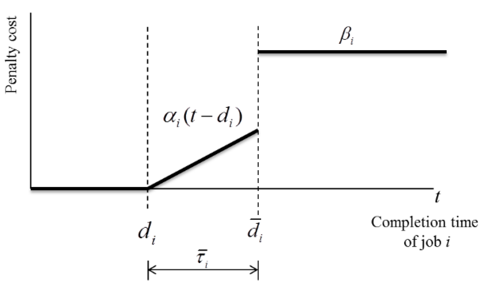
In many manufacturing or service industries, customers may specify maximum allowable tardiness for their orders in purchase contracts, according to agreements with suppliers. Here, maximum allowable tardiness is a delayed time over the due date within which the customer can allow a delayed delivery. That is, customers can cancel their orders and/or request compensation for damages for the unfulfilled contract when the delayed time over the due date exceeds maximum allowable tardiness. A typical example can be found in the semiconductor market, where the power of major customers such as Apple or Dell is continuously increasing in the supply chain. If a delivery for a customer’s order is late for its due date, and within the maximum allowable tardiness, the supplier pays a penalty fee or gives price discounts to the customer for the late fulfillment of the orders. Usually, the later the order is fulfilled, the higher the penalty cost. Customers in the semiconductor market usually allow one or two weeks lateness over the due dates, although allowable tardiness mainly depends on the levels of their safety stocks. If the delivery is late over the maximum allowable tardiness, customers will cancel their orders and try to find other suppliers. In this case, the supplier may have to scrap the products of the canceled orders if there are no other customers to buy the products. This happens occasionally if the products of cancelled orders are non-commodity ones, such as application process (AP) chips or multi-chip-package chips. Thus, it is critical to have competitiveness in meeting the due dates of customers’ orders in the semiconductor manufacturing industry. According to [
1], individual job release times and due dates, combined with other processing environment characteristics of a semi-conductor manufacturing facility, have formed a complex job shop scheduling problem (JSP). Mason et al. [
2] also mentioned that massive penalties for not satisfying the due date of orders require semiconductor manufacturers to control their manufacturing facilities efficiently. So far, most research on the job shop scheduling problem has been focused on the makespan criterion. However, due date related performance is becoming more significant in the make-to-order manufacturing environment nowadays [
3].
In this study, we deal with the job shop scheduling problem with maximum allowable tardiness (JSP-MAT). In the job shop, any job consisting of a number of different operations could be performed by different machines. We were inspired by a real factory problem in a semiconductor chip packaging and test process in Korea. In the test process, three kinds of tests are performed: burn-in tests, electrical power-consumption tests, and functional speed tests. Among these tests, the electrical power consumption test and functional speed test consist of multiple routes, with sub-steps which are determined by the product types and the former test results. Furthermore, customers designate, both a normal shipping date, and a final shipping date (with late penalty) for the ordering contract. This production process can be modeled as a job shop with maximum allowable tardiness (MAT).
We study the JSP-MAT with the objective of minimizing the total penalty cost, where two kinds of penalty costs are considered, i.e., tardiness penalty costs for allowable tardy jobs, and lost-sale penalty costs for cancelled jobs. The JSP-MAT is a special case of the job shop scheduling problem, which is one of the most studied problems in the scheduling area.
Although there have been lots of studies on dispatching rules for job shop scheduling, with the objective of minimizing total tardiness, there is a lack of research works considering the two penalty costs. Furthermore, some optimal solution tools, such as CPLEX, have the limitation of not providing the optimal solutions for the large-sized job shop scheduling problem within a reasonable time. In many industries, operation managers require practical tools that can solve a large-sized problem quickly, rather than using time-consuming optimization tools. In addition, existing dispatching rules have a limitation in improving the performance of job shop operations, because fixed priorities, determined by a certain dispatching rule, are assigned to all operations so that they offer the same solution for the same problem. To overcome these limitations, we developed probabilistic dispatching rules to solve the JSP-MAT, with the objective of minimizing the total penalty cost. The proposed rules are an extended version of earliest due date (EDD), modified due date (MDD), SLACK, original cost over time (COVERT), and apparent tardiness cost (ATC), which are known to work well for the job shop tardiness scheduling problem, by considering lost-sale penalty costs as well as tardiness costs, in order to set the priority of jobs to be scheduled in a probabilistic manner.
2. Previous Works
In general, three kinds of solution approaches to the job shop scheduling problem exist. First, meta-heuristics, such as genetic algorithms, simulated annealing algorithms, and a tabu search have been proposed to obtain near-optimal solutions efficiently for large-scale problem instances. Second, exact algorithms, such as Lagrangian relaxation approaches, queuing network models, and branch-and-bound methods have been proposed to solve the problem to optimality. Lastly, dispatching rules have been developed to obtain good solutions quickly for practical use. Holthaus and Rajendran [
4] classified the dispatching rules in a job shop into four categories: (1) process-time based rules, (2) due-date based rules, (3) combination rules, and (4) rules that are neither process-time based nor due-date based. For an extensive literature review of the job shop scheduling problem, refer to Blazewicz et al. [
5].
There have been research works for the JSP in semiconductor manufacturing. For example, Gupta and Sivakumar [
3] reviewed the job shop scheduling techniques in semiconductor manufacturing, including dispatching rules, mathematical programming techniques, search methods, and AI techniques. Mönch et al. [
6] discussed several problems and solution techniques in semiconductor manufacturing, and addressed the challenging issues in scheduling semiconductor manufacturing operations. Several researchers mentioned the necessity, or importance, of the research of semiconductor job shop scheduling. For example, Essafi et al. [
7] reported that research works dealing with the minimization of due date related objectives in job-shops are very scarce, despite the increasing importance of customer service in terms of meeting due dates. Zhang and Wu [
8] also mentioned that the research on the total weighted tardiness objective is comparatively scarce, because this objective function is more difficult and complex to optimize. Due date related performance is becoming more significant in the make-to-order manufacturing environment nowadays [
8].
Various algorithms have been proposed to solve the JSP, with the objective of minimizing total tardiness. Singer and Pinedo [
9] proposed branch and bound algorithms, having two types of branching schemes for minimizing the total weighted tardiness in job shops. Pinedo and Singer [
10] proposed a shifting bottleneck heuristic to minimize the total weighted tardiness in a job shop. To resolve the problem efficiently, in the proposed heuristic they applied a decomposition concept to break down the job shop into a number of single-machine subproblems. Asano and Ohta [
11] dealt with a JSP to minimize the total weighted tardiness, with job-specific due dates and delay penalties. To resolve the problem, they proposed a heuristic algorithm based on the tree search procedure. Mattfeld and Bierwirth [
12] proposed a genetic algorithm for JSPs, with release and due-dates, and with various tardiness criteria (e.g., weighted mean tardiness, maximum tardiness of jobs, and weighted number of tardy jobs) as objectives. Furthermore, Mason et al. [
2] investigated three rescheduling strategies for complex job shops, such as semiconductor wafer fabs having dynamic and uncertain environments, with the objective of minimizing order total weighted tardiness. Mason et al. [
1] presented a mixed integer programming (MIP) heuristic, solved by CPLEX, to minimize total weighted tardiness in a complex job shop. In order to evaluate the proposed method, they compared it with a modified shifting bottleneck heuristic and various dispatching rules. De Bontridder [
13] also addressed a JSP with release times, positive end-start time lags, and a general precedence graph under the objective of minimization of the total weighted tardiness. To resolve the problem, they proposed a tabu search algorithm to search for the order in which the operations were processed on each machine. Chiang and Fu [
14] reviewed eighteen dispatching rules for the JSP with due data-based objectives and proposed a new dispatching rule, having a balanced performance when more than one objective is considered. Essafi et al. [
7] addressed the job-shop problem with the objective of minimizing the total weighted tardiness, considering release dates and due dates. To resolve the problem, they proposed a genetic local search algorithm. Zhou et al. [
15] also dealt with a JSP to minimize weighted tardiness. They proposed a hybrid framework, integrating a genetic algorithm (GA) and four dispatching rules, i.e., weighted COVERT, Rachamadagu and Morton (RandM), weighted shortest processing time (SPT), and EDD. In their scheduling framework, the first operation of each machine was determined by the GA, and the remaining operations are allocated to the machines by a dispatching rule. They showed that the proposed hybrid framework functioned well, regardless of different levels of due-date tightness. Recently, Zhang and Wu [
8] dealt with a JSP with the objective of minimizing total weighted tardiness. To solve the problem more effectively, they revised a simulated annealing algorithm with a block-based neighborhood structure. Chen and Matis [
16] proposed the weighted biased modified rule (WBMR) to minimize the mean weighted tardiness of jobs in a job shop. They showed that WBMR outperformed other traditional rules at various congesting and due-date tightness levels.
However, to the best of our knowledge, the JSP with maximum allowable tardiness (JSP-MAT) has not yet been studied, while there are only a few studies for the single machine scheduling problem with maximum allowable tardiness, including [
17,
18,
19,
20,
21]. In this study, we deal with the JSP-MAT. The objective of the problem is to minimize the total penalty cost consisting of two kinds of penalty costs, i.e., tardiness penalty costs for allowable tardy jobs, and lost-sale penalty costs for cancelled jobs. Due to the dynamic characteristic of manufacturing lines, the scheduling problem should be solved very quickly, so dispatching rules are commonly used in practice [
22]. In this study, we propose dispatching rules with a probability scheme for the JSP-MAT. This paper is organized as follows: In the next section, we declare the integer programming model of the JSP-MAT. The probabilistic dispatching rules for the job shop scheduling are presented in
Section 3. In
Section 4, we report the performance of the suggested rules through computational experiments. Finally,
Section 5 concludes the paper with a short summary.
4. Dispatching Rules
4.1. Extend Dispatching Rules
In many industries, operation managers require practical tools that can solve large-sized operational problems quickly, rather than using time-consuming optimization tools. In this paper, we suggest several practical dispatching rules for the JSP-MAT, which can be implemented in the production planning and scheduling process at actual manufacturing facilities. Dispatching rules are used to determine the job sequence in which jobs should be worked. Various dispatching rules have been developed for the JSP [
23,
24], and five dispatching rules (EDD, MDD, SLACK, COVERT, and ATC) are most widely used in practice, and are known to perform better than others, in terms of the total tardiness criterion [
14,
25,
26,
27]. In this section, we extend these five dispatching rules to improve their performance for the JSP-MAT. For this, we introduce additional notation, as below:
| |
| total processing time of job i |
| average total processing time of the remaining jobs |
| total remaining processing time of job i |
(1) EEDD
In the earliest due date (EDD) rule, jobs with earlier due dates have higher priorities and are processed before those with later due dates. The EDD rule that considers the weight of tardiness penalty cost can be represented by EDD: . For the JSP-MAT, the EDD rule can be extended by considering both the weight of tardiness penalty cost and lost-sale penalty cost. This rule is named the extended EDD (EEDD) rule in this study, and given as follows: EEDD: , where is a set of unselected jobs.
Note that is used instead of in the proposed rule because has the same measure as , i.e., a cost per unit time.
(2) EMDD
The modified due date (MDD) rule was originally suggested by [
28] for the JSP. In this rule, the modified due date of a job is defined as the larger value of the due date of the job and the earliest possible completion time of the job. The MDD rule selects the job with the least modified due date among the unselected jobs to be processed next. The modified due dates of jobs are updated each time a new job is selected because the earliest possible completion times of the unselected jobs depend on those of selected ones. In this regard, the MDD rule is called the dynamic dispatching rule. The MDD rule that considers the weight of tardiness penalty cost can be represented by
. Then the extended MDD (EMDD) rule that considers both the weight of tardiness penalty cost and lost-sale penalty cost can be represented as follows:
In the EMDD rule, priorities of jobs to be selected are determined by the three different criteria, according to the range of their earliest possible completion times. The basic concept of the EMDD rule is that a job has one of three different types of modified due dates according to the range of the earliest possible completion time of the job. In the case that the earliest possible completion time of job i is not greater than , represents , i.e., the modified due date of job i, while replaces it when the earliest possible completion time exceeds the due date but not the cancellation deadline. Note that is usually less than because in general. On the other hand, a very large value V is assigned to the modified due date when the job cannot help being cancelled. Once a job turns out to be cancelled, we assign it the lowest scheduling priority so as not to consider it any longer.
(3) ESLACK
In the SLACK rule, the job with the least slack time has the highest priority. The slack time of a job is defined as the maximum available time to delay the completion of the job without violating its due date. The job slack time is computed as the difference between the job due-date and the earliest possible completion time for the job. As with the MDD rule, the SLACK rule is also a dynamic dispatching rule, because the job slack time is not static, but should be updated each time a new job is selected for processing. The SLACK rule that considers the weight of tardiness penalty cost is represented by SLACK:
. Then the Extended SLACK (ESLACK) rule that considers both the weight of tardiness penalty cost and lost-sale penalty cost can be represented as follows:
(4) ECOVERT
The original cost over time (COVERT) priority index represents the expected tardiness cost per unit of imminent processing time, or cost over time [
23]. The COVERT rule is a ratio-based dispatching rule, which combines the SLACK rule and the shortest processing time (SPT) rule. It puts the job with the largest COVERT ratio in the first position of the job sequence. The COVERT ratio of a job is computed by dividing a derived urgency ratio of the job by the pseudo-processing time of the job. It is known that it performs well on due date-based objectives, especially on the total tardiness measure for the JSP [
29]. The COVERT rule that considers the weight of tardiness penalty cost can be represented by COVERT:
. In COVERT,
k is a parameter, and its value is usually determined through experimental analysis. We extend the COVERT rule to ECOVERT rule by considering both the weight of tardiness penalty cost and lost-sale penalty cost as follows:
Note that the ECOVERT is different from the previous three dispatching rules proposed, in that it gives higher priorities to jobs with larger COVERT ratios. The COVERT ratio of job i, , has a value between 0 and if , and one between and if , and otherwise. Since the lost-sale penalty cost is much higher than the tardiness penalty cost, job i has larger as the possibility of the job being cancelled is increased.
(5) EATC
The apparent tardiness cost (ATC) rule was developed based on the COVERT rule for the JSP [
23]. The basic concept of the ATC rule is the same as the COVERT rule, with two main differences. First, the ATC rule uses an exponential function rather than a linear one to emphasize the role of slack. Second, the ratio is calculated by dividing the job slack by the average processing time, instead of the job processing time. The ATC that considers the weight of tardiness penalty cost can be represented by ATC:
. Here,
k is a parameter and
. Then the Extended ATC (EATC) can be represented as follows:
4.2. Probabilistic Dispatching Rules
The main disadvantage of the dispatching rules is that they always offer the same schedule for the same problem instance, because jobs with higher priorities are processed earlier in them, which however does not guarantee better solutions. To overcome this, we proposed probabilistic dispatching rules, based on the five dispatching rules proposed in the previous section. In the probabilistic dispatching rules, jobs with higher priorities are selected for processing with higher probabilities, which enables them to generate various solutions for the same problem instance. To assign a selection probability to each job, we use the softmax function denoted as
which takes a
K-dimensional vector of arbitrary real values, and produces another
K-dimensional vector with real values in the range (0, 1) that add up to 1.0. Let us consider a
K-dimensional input vector
z =
. Then
, which can be regarded as a probability that event
i occurs when the value of event
i is
. By using the softmax function, a probability that a certain event occurs increases exponentially as the value of the event increases. In this study, probabilistic versions for the five dispatching rules proposed are denoted, respectively, as PEEDD, PEMDD, PESLACK, PECOVERT, and PEATC. Among these, PEMDD can be represented as below:
In the PEMDD rule, Prob(i) represents the probability that job i is selected for processing. To select a job for dispatching, we sort the values of all jobs in the unselected job set in a non-increasing order, and let [i] indicate the index of the i-th job in the sorting sequence. Then, job [k] is selected if , for , where U(0, 1) is a randomly selected real value with a range [0,1]. Finally, the best solution is selected for scheduling among prescribed number of replicates obtained by applying this rule iteratively.
The other four probabilistic dispatching rules PEEDD, PESLACK, PECOVERT, and PEATC can be represented in the same manner as PEMDD.
5. Computational Experiments
To test the performance of the suggested dispatching rules, we randomly generated 300 test instances varying the numbers of jobs, due-date tightness, and range of allowable tardiness: five levels for the number of jobs, three levels for the due-date tightness, and 20 replications for each combination. Note that currently open data sets of job shop problems are not suitable for this study because they do not contain information about the maximum allowable tardiness and the related penalty cost. Instead, we generated suitable data sets for this study based on a statistical specification from a real factory of a semiconductor chip packaging and test process in Korea. In the semiconductor chip test process, three kinds of tests are performed: burn-in tests, electrical power-consumption tests, and functional speed tests. Among these tests, the electrical power consumption test and functional speed test consist of multiple routes, with sub-steps according to the production process of the product types and their former test results. We modified the statistical specification to protect the company’s industrial property right, without loss of generality, and published the full data set publicly [
30].
In the generated problem, we assumed the following:
- (1)
Set-up times are included in the processing times.
- (2)
Each machine can perform at most one job at a time.
- (3)
Each job can be processed only on one machine at a time, without preemption.
- (4)
Each operation has a deterministic processing time.
- (5)
The transportation time between different machines can be neglected.
- (6)
No machine breakdown or maintenance happens.
In each problem instance, relevant data were generated as follows. Here, DU(a, b) and U(a, b) denote random numbers generated from the discrete and continuous uniform distributions, with a range (a, b), respectively.
- (1)
The number of jobs used in computational experiments is 10, 20, 30, 40, or 50.
- (2)
The number of machines is generated considering the number of jobs as follows: 3·N/10.
- (3)
The number of operations for each job is randomly generated with DU(1, 10). If the number of operations is bigger than the number of machines, then the number of operations is set to the number of machines.
- (4)
The processing time of each operation is randomly generated with DU(1, 20).
- (5)
The machine to take each operation of a job is randomly assigned.
- (6)
The due date of each job is randomly determined between 1 and 5 times of the total processing time of each job. That is, it is set to , where is a random number between 1 and 5.
- (7)
There are three levels of allowable due date tightness: loose, normal, and tight. For this, cancellation deadline of job i is set to , where is a factor for controlling the range of allowable due date tightness and it is set to U(1, 2) for tight allowable due dates, U(1, 3) for normal ones, and U(1, 4) for loose ones. Note that larger generates bigger allowable due date tardiness.
- (8)
Tardiness penalty cost per unit time for job i, i.e., αi, was set to U(1.0, 5.0)
- (9)
Lost-sale penalty cost of job i is generated as follows: , where η is a random value between 5 and 15.
First, we compared five existing dispatching rules (i.e., EDD, SLACK, MDD, COVERT, and ATC) with our extended ones (i.e., EEDD, ESLACK, EMDD, ECOVERT, and EATC).
Table 1 summarizes the relative deviation index (RDI) values of solutions obtained by each rule for each number of jobs. Here the RDI of solution s is calculated as below:
Note that the range of RDI is between 0 and 1, where 0 and 1 denote the best and the worst solutions, respectively.
The results of
Table 1 tell us the following: first, most of the extended dispatching rules gave better performance than the original dispatching rules, although the performance of EEDD was not better than that of EDD. Second, overall, ECOVERT outperformed the other rules, irrespective of the number of jobs and levels of due date tightness.
Table 2 shows the number of best solutions (NBS) found by each rule. In
Table 2, we can also see similar results: first, many of the extended dispatching rules, such as EMDD, ECOVERT, and EATC, gave better results than the original dispatching rules. However, EEDD and ESLACK gave slightly worse results than EDD and SLACK. Second, ECOVERT found a total of 126 best solutions, which was overwhelming in comparison with the others. ECOVERT always found the highest number of best solutions among all the rules.
Next, we compared the extended dispatching rules with the probabilistic dispatching rules (i.e., PEEDD, PEMDD, PESLACK, PECOVERT, and PEATC) and solutions from CPLEX 12.1, the commercial optimization solver. In CPLEX, we set the time limit to solve the JSP-MAT as 200 s, and set the parameter mipemphasis as CPXMIPEMPHASIS_FEASIBILITY to obtain a good and feasible solution rather than an optimal solution within the short time limit. In ECOVERT and EATC rules, the parameter k was set to 2. For each probabilistic dispatching rule, the best solution was selected among 1000 replicates, obtained by applying each rule iteratively.
Table 3 shows the NBS found by each rule for each job size. Overall, the probabilistic dispatching rules found more NBS than the extended dispatching rules did. As the number of jobs increased, it seemed that NBS of most rules became worse. However, PECOVERT and PESLACK gave the best solutions, irrespective of the number of jobs. It was also observed that EDD based rules, such as EEDD and PEEDD, gave the worse performance.
Table 4 indicates the averages and standard deviations of RDI values for extended dispatching rules and their probabilistic rules, compared with the solutions of CPLEX 12.1. The test results in
Table 4 show that the PECOVERT rule outperformed the other rules. In terms of the solution quality, the result shows that as the number of jobs increased, the RDI values of most dispatching rules also increased, until the number of jobs was 30, which means that the number of jobs highly affected the performance of the dispatching rules in a negative way. However, from a number above 40, those of most dispatching rules seemed to be decreasing. CPLEX’s solutions outperformed the other dispatching rules’ solutions when the number of jobs was 10 or 20. However, CPLEX’s RDI values tended to increase rapidly as the number of jobs increased. Especially when the number was over 40; it was relatively bad compared to those of ECOVERT or PECOVERT. It was also observed that the degree of due date tightness did not seem to affect the performance of solutions of the dispatching rules. Overall, the probabilistic extended dispatching rules were much better than the extended dispatching rules. Among the suggested rules, PECOVERT and PESLACK were the best, followed by PEATC. In particular, the PECOVERT rule gave the best solutions, irrespective of the number of jobs. The outstanding performance of the PECOVERT rule became more evident when the job size became larger, as shown in
Figure 2. In summary, we could see that PECOVERT gave a robust performance, and its solution quality was also good when compared to the solutions of CPLEX, in particular, when the number of jobs was over 30.
To see if there was any statistically significant difference in the performances of the dispatching rules and CPLEX, statistical comparison tests were carried out. Prior to the comparison between two methods, the normality test with significance level 0.01 was carried out. As a result, normality was not guaranteed for all cases, so that a non-parametric method for the comparison of two groups, the Wilcoxon signed rank test with significance level 0.01, was carried out instead of paired
t-tests. As per the summarized results shown in
Table 5, we see that the rank is determined as follows PECOVERT > PESLACK > PEATC > CPLEX, ECOVERT, PEMDD > EATC > ESLACK > PEEDD > EMDD > EEDD. Overall, the proposed PECOVERT rule gave the best performance among tested dispatching rules. We also found that there was no significant difference in the results of the following two rules: CPLEX, ECOVERT, and PEMDD.
To assess the efficiency of PECOVERT and CPLEX, the computational times of PECOVERT and CPLEX for 300 test problems are reported in
Table 6. The test results show that CPLEX found optimal solutions for all the 10-job test instances within 0.5 s. However, the computational times of CPLEX exponentially increased as the number of jobs increased. CPLEX frequently timed out (200 s) in solving the large-sized problems. While the computational times of PECOVERT are very short (about 2 s or less), even in the cases with more than 40 jobs. This means that PECOVERT efficiently solves the large-sized JSP-MAT within a reasonable time, in practice.
6. Conclusions
In this study, we dealt with the JSP-MAT, with the objective of minimizing tardiness penalty costs, consisting of penalty costs for allowable tardy jobs and those for cancelled jobs. We proposed probabilistic dispatching rules for the JSP-MAT by extending five well-known dispatching rules for the JSP, and adding a probabilistic concept into them. We conducted computational experiments to test the performance of the proposed rules. The test results showed that the extended dispatching rules outperformed the original dispatching rules, and the probabilistic dispatching rules work better than the extended dispatching rules. Among the proposed rules, PECOVERT showed the best performance; its solution quality was as good as CPLEX, despite its fast execution. Compared to CPLEX, the larger the number of jobs, the worse the CPLEX solution was, while PECOVRT gave stable and good solutions.
The suggested dispatching rules, especially PECOVERT, can be used as a viable tool for machine scheduling in the manufacturing industries which have penalty costs for order cancellation due to tardiness, such as the semiconductor manufacturing industry. They also can be used to develop an order promising procedure in the semiconductor business. The demand management system of a semiconductor manufacturing company receives orders from customers, and gives back the information on the estimated completion times and the quantities of products that can be shipped within due dates. After several runs of order promising negotiation, the product quantities and the due dates of the orders are confirmed, and only the confirmed orders will be processed by a production system. During the negotiation, the JSP-MAT can be solved using the suggested dispatching rules to estimate the completion times of the orders, and to decide whether the orders should be accepted or not, by considering the maximum allowable tardiness from the customers.
In conclusion, although the probabilistic extended dispatching rules do not outperform the solutions of a commercial optimization solver in all cases, we believe that they could give satisfactory results, as good as the optimization solver’s solutions. Furthermore, due to the simplicity and speed of the probabilistic extended dispatching rules, they could be easily used in practice and in simulation models of semiconductor production scheduling. For future research, it is necessary to study modifications and adaptations of more sophisticated heuristics or dispatching rules, which are known as relatively good algorithms for the single machine total tardiness scheduling problem, for further research of the JSP-MAT.


