Static Deformation-Compensation Method Based on Inclination-Sensor Feedback for Large-Scale Manipulators with Hydraulic Actuation

Abstract

Modern large-scale manipulators with hydraulic actuation like mobile concrete pump manipulators are increasingly used in industrial, construction, and other fields. Due to the large span of these manipulators, the static deformation accumulation to the endpoint has seriously affected the precise control of the endpoint. In this paper, we propose a static deformation-compensation method based on inclination sensor feedback for large-scale manipulators to reduce the deviation of the endpoint. Compared with the finite element method, this method does not need to consider many boundary conditions that are uncertain for flexible manipulators in most situations. It has appropriate accuracy and is universal for large-scale manipulators of different sizes and working under different loads. Based on a 24m-3R mobile concrete pump manipulator, the parametric simulation is carried out. The reliability of the static deformation-compensation method is verified, and the error is analyzed. The validity of the static deformation-compensation method is verified by comparing the theoretical endpoint position with the actual endpoint position after static deformation compensation. The compensation error under different loads is obtained, and the universality of the compensation method for different loads is verified.

1. Introduction

Modern large-scale manipulators are increasingly used in industrial, construction, and other fields. With the increase in the operational speed requirements of large-scale manipulators and the demand for lightweight design, the flexibility of these manipulators have gradually increased. Compared to the conventional heavy and bulky manipulators, flexible link manipulators have the potential advantage of lower cost, larger working volume, faster operational speed, larger payload-to-manipulator-weight ratio, smaller actuators, lower energy consumption, better maneuverability, better transportability, and safer operation due to reduced inertia [1,2,3,4]. The concepts of modern light-weight construction enable the large-scale manipulators like mobile concrete pump manipulators with extended operating range and less static load. However, due to the reduced weight, the elasticity of the construction elements has a significant influence on the precise positioning of the endpoint [5,6]. The influence of large-scale manipulators’ static deformation on the precise control of the endpoint cannot be ignored anymore [6,7].

The research on the motion control of the engineering manipulator has made good progress [8,9,10,11,12,13,14,15,16,17]. Many researchers have studied the control of the endpoint trajectory of the mobile concrete pump manipulator. Most of them considered the manipulator as rigid. Although the control of the endpoint trajectory was realized, there are still positioning errors (deviation of the endpoint) due to static deformation [18,19,20]. Despite the length of the mobile concrete pump manipulator ranging from 24 m to 53 m that are widely used now, the demand for the length of the mobile concrete pump manipulator will be higher with the development of the construction level and the influence of static deformation will be more serious.

In the literature, there are many types of research on the modeling of flexible multi-body systems. The existing methods are well developed and are presented in several textbooks, e.g., Bremer, Shabana, and many others [21]. For large-scale manipulators like mobile concrete pump manipulators, hydraulic actuators comprising hydraulic cylinders and valves are commonly used. Their dynamic behavior and the nonlinear characteristics have to be considered in the controller design. Henikl et al. and Lambeck et al. studied the combination of flexible multi-body systems and hydraulic actuators [22,23,24]. Zimmert et al. presented a control design considering the infinite-dimensional model of a flexible turntable ladder [25].

Many researchers have studied different schemes for modeling flexible link manipulators. Links are subjected to torsion, bending, and compression. The main concern is bending. For bending one may often use the Euler–Bernoulli equation, which ignores shearing and rotary inertia effects. These two effects may be incorporated using a Timoshenko beam element, which always is used if the beam is short relative to its diameter. However, since links may be considered as being rigid [26], in most models of flexible manipulators Euler–Bernoulli beams are used. In the literature [27,28], there are many well-established dynamic models in which three main modeling methods of the flexible link manipulators are the assumed mode method (AMM), the finite element method (FEM), and the lumped parameter model. AMM and FEM use either the Lagrangian formulation or the Newton–Euler recursive formulation.

The flexibility of the link is usually represented by a truncated finite modal series in terms of spatial mode eigenfunctions and time-varying mode amplitudes in assumed mode model (AMM) formulation. This method’s main disadvantage is the difficulty in finding modes for links with non-regular cross sections and multi-link manipulators [29]. Using the law of conservation of momentum, the Lagrangian principle was utilized to model the dynamic function of the space flexible manipulator incorporating the assumed modes method in Deng-Feng’s research [30]. Subudhi and Morris [31] presented a dynamic modeling technique for a manipulator with multiple flexible links and flexible joints based on a combined Euler–Lagrange formulation and assumed modes method. Then, they controlled the system by formulating a singularly perturbed model and used it to design a reduced-order controller. In the finite element method (FEM), the elastic deformations are analyzed by assuming a known rigid body motion and later superposing the elastic deformation with the rigid body motion [32,33,34,35,36,37]. In order to solve a large set of differential equations derived by the finite element method, a lot of boundary conditions have to be considered, which are, in most situations, uncertain for flexible manipulators [38]. Using the assumed mode method to derive the equations of motion of the flexible manipulators, only the first several modes are usually retained by truncation and the higher modes are neglected. The lumped parameter model is the simplest one for analysis purposes; the manipulator is modeled as a spring and mass system, which does often not yield sufficiently accurate results [39,40,41]. Zhu et al. [42] employed a lumped model to simulate the tip position tracking control of a single-link flexible manipulator. Raboud et al. [43] showed the existence of multiple equilibrium solutions under a given load condition by studying the stability of very flexible cantilever beams.

Some researchers have paid attention to the static deformation of large-scale manipulators. Most of them are based on the application of finite element method (FEM) in the static deformation of flexible manipulators. Lee et al. reduced the endpoint deviation of the mobile concrete pump manipulator by 30% compared with steel structures by using carbon fiber material in the last link [44]. In order to better improve the trajectory tracking accuracy of the working platform at high altitude, Qing Hui Yuan considered the elastic deformation of the manipulator and the influence of vibration on the trajectory tracking control and introduces the deformation compensation strategy to eliminate the influence [45]. Xia Jijun et al., based on finite element deformation analysis under the actual load conditions of the mobile concrete pump manipulator system, established an expert database of full position and orientation deformation compensation of the manipulator and applied it to the trajectory control of the endpoint. The position deviation of the endpoint could be controlled within ±15 cm [46]. Zhao Xin et al. obtained the deformation compensation model of the manipulator and the vehicle body through the deformation analysis of the whole concrete pump truck under the full working condition, established the kinematics model of the concrete pump truck after the deformation compensation and used the control method of the cerebellar model neural network in the motion control, and well solved the dynamic detection and trajectory control of the manipulator position and orientation [47]. Wang Xiaoming et al. used finite element simulation to establish the data model of the deformation of the manipulator during the trajectory control process. Then, the BP neural network model was used to establish the deformation compensation algorithm, and the deformation law of the manipulator was obtained [48]. Pan Daoyuan et al. used FEM to analyze the variation of the acceleration of the manipulator and the force applied on the manipulator in different positions and orientations, and determined their influence on the deformation [49]. These studies have made some achievements and have made great progress in the deformation compensation of mobile concrete pump manipulators. However, these studies are based on the prototype studied by them, such as Xia Jijun et al. with Zoomlion 52m-6RZ concrete pump truck (RZ manipulator folding structure) as the research prototype [46]. Wang Xiaoming, Zhao Xin et al., and Pan Daoyuan et al. all built finite element simulation results databases based on their respective experimental prototypes [47,48,49]. All of the above studies needed to establish an accurate simulation model and needed to consider a lot of boundary conditions. The amount of calculation was very large, and the methods used to develop the prototype were not universal and thus are difficult to use in practical applications.

In this paper, we propose a static deformation-compensation method for large-scale manipulators based on inclination sensor feedback. Compared with the finite element method, this method does not need to consider many boundary conditions that are uncertain for flexible manipulators in most situations. It has appropriate accuracy and is universal for large-scale manipulators of different sizes and working under different loads.

2. The Structure and the Forward Kinematic Model of the Mobile Concrete Pump Manipulator

2.1. Structure of the Mobile Concrete Pump Manipulator

The mobile concrete pump manipulator is a multi-degree of freedom manipulator system. This paper takes the mobile concrete pump manipulator with three links as an example to explain the static deformation-compensation method. Its main components are rotation base, 1st joint, 1st link, 2nd joint, 2nd link, 3rd joint, 3rd link, and the concrete discharge hose. Given that the concrete discharge hose has little capacity to bear the load of concrete, it is only used as the concrete discharge guide, ignoring its degree of freedom. It is a manipulator composed of four joints, each link of which is a long-scale flexible link.

During the process of concrete placing during construction, the manipulator produces a large elastic deformation caused by complex stress due to the influence of gravity on the manipulator, the pumping concrete load, the concrete flow impact, and other factors. Due to the large span of the mobile concrete pump manipulator, the deformation accumulation to the end outlet has seriously affected the concrete placing accuracy. The elastic deformation varies in different positions and orientations. Figure 1 shows a structural diagram of the mobile concrete pump manipulator.

2.2. Forward Kinematics Model of the Mobile Concrete Pump Manipulator

In order to study the influence of the joint compensation angle on the position of the endpoint, the relationship between the joint angle change of each joint and the position and orientation of the endpoint is established based on the D–H matrix (Denavit–Hartenberg Matrix) method. As shown in Figure 2, D–H coordinate system is established for the mobile concrete pump manipulator.

The distance from the rotation axis of the rotation base to the rotation axis of the 1st link is negligible compared with the length of the whole manipulator (24 m), so let the origin of the rotation base coordinate system T₁ coincide with the origin of the 1st link coordinate system T₂. The base coordinate system T₀, the rotation base coordinate system T₁, the 1st link coordinate system T₂, the 2nd link coordinate system T₃, the 3rd link coordinate system T₄, and the end coordinate system T₅ is established. According to the D–H matrix method, the homogeneous coordinate transformation matrix is calculated. The joint angle ${\mathsf{\theta }}_0{\mathsf{\theta }}_1{\mathsf{\theta }}_2{\mathsf{\theta }}_3$ is positive clockwise and negative counterclockwise:

$${}_1{}^0\mathrm{T}=\left[\begin{array}{cc}\begin{array}{cc}{c}_0& -s_0\\ s_0& c_0\end{array}& \begin{array}{cc}0& 0\\ 0& 0\end{array}\\ \begin{array}{cc}0& 0\\ 0& 0\end{array}& \begin{array}{cc}1& 0\\ 0& 1\end{array}\end{array}\right]{}_2{}^1\mathrm{T}=\left[\begin{array}{cc}\begin{array}{cc}{c}_1& -s_1\\ 0& 0\end{array}& \begin{array}{cc}0& 0\\ -1& 0\end{array}\\ \begin{array}{cc}{s}_1& c_1\\ 0& 0\end{array}& \begin{array}{cc}0& 0\\ 0& 1\end{array}\end{array}\right]$$

$${}_3{}^2\mathrm{T}=\left[\begin{array}{cc}\begin{array}{cc}{c}_2& -s_2\\ s_2& c_2\end{array}& \begin{array}{cc}0& l_1\\ 0& 0\end{array}\\ \begin{array}{cc}0& 0\\ 0& 0\end{array}& \begin{array}{cc}1& 0\\ 0& 1\end{array}\end{array}\right]{}_4{}^3\mathrm{T}=\left[\begin{array}{cc}\begin{array}{cc}{c}_3& -s_3\\ s_3& c_3\end{array}& \begin{array}{cc}0& l_2\\ 0& 0\end{array}\\ \begin{array}{cc}0& 0\\ 0& 0\end{array}& \begin{array}{cc}1& 0\\ 0& 1\end{array}\end{array}\right]{}_5{}^4\mathrm{T}=\left[\begin{array}{cc}\begin{array}{cc}1& 0\\ 0& 1\end{array}& \begin{array}{cc}0& l_3\\ 0& 0\end{array}\\ \begin{array}{cc}0& 0\\ 0& 0\end{array}& \begin{array}{cc}1& 0\\ 0& 1\end{array}\end{array}\right]$$

$${}_5{}^0\mathrm{T}={\left(\begin{array}{cccc}\begin{array}{c}{\mathbf{c}}_{\mathbf{3}}({\mathbf{c}}_{\mathbf{0}}{\mathbf{c}}_{\mathbf{1}}{\mathbf{c}}_{\mathbf{2}}-{\mathbf{c}}_{\mathbf{0}}{\mathbf{s}}_{\mathbf{1}}{\mathbf{s}}_{\mathbf{2}})-{\mathbf{s}}_{\mathbf{3}}({\mathbf{c}}_{\mathbf{0}}{\mathbf{c}}_{\mathbf{1}}{\mathbf{s}}_{\mathbf{2}}+{\mathbf{c}}_{\mathbf{0}}{\mathbf{c}}_{\mathbf{2}}{\mathbf{s}}_{\mathbf{1}})\\ {\mathbf{c}}_{\mathbf{3}}({\mathbf{c}}_{\mathbf{1}}{\mathbf{c}}_{\mathbf{2}}{\mathbf{s}}_{\mathbf{0}}-{\mathbf{s}}_{\mathbf{0}}{\mathbf{s}}_{\mathbf{1}}{\mathbf{s}}_{\mathbf{2}})-{\mathbf{s}}_{\mathbf{3}}({\mathbf{c}}_{\mathbf{1}}{\mathbf{s}}_{\mathbf{0}}{\mathbf{s}}_{\mathbf{2}}+{\mathbf{c}}_{\mathbf{2}}{\mathbf{s}}_{\mathbf{0}}{\mathbf{s}}_{\mathbf{1}})\\ {\mathbf{c}}_{\mathbf{3}}({\mathbf{c}}_{\mathbf{1}}{\mathbf{s}}_{\mathbf{2}}+{\mathbf{c}}_{\mathbf{2}}{\mathbf{s}}_{\mathbf{1}})+{\mathbf{s}}_{\mathbf{3}}({\mathbf{c}}_{\mathbf{1}}{\mathbf{c}}_{\mathbf{2}}-{\mathbf{s}}_{\mathbf{1}}{\mathbf{s}}_{\mathbf{2}})\\ \mathbf{0}\end{array}& \begin{array}{c}-{\mathbf{c}}_{\mathbf{3}}({\mathbf{c}}_{\mathbf{0}}{\mathbf{c}}_{\mathbf{1}}{\mathbf{s}}_{\mathbf{2}}+{\mathbf{c}}_{\mathbf{0}}{\mathbf{c}}_{\mathbf{2}}{\mathbf{s}}_{\mathbf{1}})-{\mathbf{s}}_{\mathbf{3}}({\mathbf{c}}_{\mathbf{0}}{\mathbf{c}}_{\mathbf{1}}{\mathbf{c}}_{\mathbf{2}}-{\mathbf{c}}_{\mathbf{0}}{\mathbf{s}}_{\mathbf{1}}{\mathbf{s}}_{\mathbf{2}})\\ -{\mathbf{c}}_{\mathbf{3}}({\mathbf{c}}_{\mathbf{1}}{\mathbf{s}}_{\mathbf{0}}{\mathbf{s}}_{\mathbf{2}}+{\mathbf{c}}_{\mathbf{2}}{\mathbf{s}}_{\mathbf{0}}{\mathbf{s}}_{\mathbf{1}})-{\mathbf{s}}_{\mathbf{3}}({\mathbf{c}}_{\mathbf{1}}{\mathbf{c}}_{\mathbf{2}}{\mathbf{s}}_{\mathbf{0}}-{\mathbf{s}}_{\mathbf{0}}{\mathbf{s}}_{\mathbf{1}}{\mathbf{s}}_{\mathbf{2}})\\ {\mathbf{c}}_{\mathbf{3}}({\mathbf{c}}_{\mathbf{1}}{\mathbf{c}}_{\mathbf{2}}-{\mathbf{s}}_{\mathbf{1}}{\mathbf{s}}_{\mathbf{2}})-{\mathbf{s}}_{\mathbf{3}}({\mathbf{c}}_{\mathbf{1}}{\mathbf{s}}_{\mathbf{2}}+{\mathbf{c}}_{\mathbf{2}}{\mathbf{s}}_{\mathbf{1}})\\ \mathbf{0}\end{array}& \begin{array}{c}{\mathbf{s}}_{\mathbf{0}}\\ -{\mathbf{c}}_{\mathbf{0}}\\ \mathbf{0}\\ \mathbf{0}\end{array}& \begin{array}{c}{\mathbf{l}}_{\mathbf{2}}({\mathbf{c}}_{\mathbf{0}}{\mathbf{c}}_{\mathbf{1}}{\mathbf{c}}_{\mathbf{2}}-{\mathbf{c}}_{\mathbf{0}}{\mathbf{s}}_{\mathbf{1}}{\mathbf{s}}_{\mathbf{2}})+{\mathbf{l}}_{\mathbf{3}}\left({\mathbf{c}}_{\mathbf{3}}\right({\mathbf{c}}_{\mathbf{0}}{\mathbf{c}}_{\mathbf{1}}{\mathbf{c}}_{\mathbf{2}}-{\mathbf{c}}_{\mathbf{0}}{\mathbf{s}}_{\mathbf{1}}{\mathbf{s}}_{\mathbf{2}})-{\mathbf{s}}_{\mathbf{3}}({\mathbf{c}}_{\mathbf{0}}{\mathbf{c}}_{\mathbf{1}}{\mathbf{s}}_{\mathbf{2}}+{\mathbf{c}}_{\mathbf{0}}{\mathbf{c}}_{\mathbf{2}}{\mathbf{s}}_{\mathbf{1}}\left)\right)+{\mathbf{c}}_{\mathbf{0}}{\mathbf{c}}_{\mathbf{1}}{\mathbf{l}}_{\mathbf{1}}\\ {\mathbf{l}}_{\mathbf{3}}\left({\mathbf{c}}_{\mathbf{3}}\right({\mathbf{c}}_{\mathbf{1}}{\mathbf{c}}_{\mathbf{2}}{\mathbf{s}}_{\mathbf{0}}-{\mathbf{s}}_{\mathbf{0}}{\mathbf{s}}_{\mathbf{1}}{\mathbf{s}}_{\mathbf{2}})-{\mathbf{s}}_{\mathbf{3}}({\mathbf{c}}_{\mathbf{1}}{\mathbf{s}}_{\mathbf{0}}{\mathbf{s}}_{\mathbf{2}}+{\mathbf{c}}_{\mathbf{2}}{\mathbf{s}}_{\mathbf{0}}{\mathbf{s}}_{\mathbf{1}}\left)\right)+{\mathbf{l}}_{\mathbf{2}}({\mathbf{c}}_{\mathbf{1}}{\mathbf{c}}_{\mathbf{2}}{\mathbf{s}}_{\mathbf{0}}-{\mathbf{s}}_{\mathbf{0}}{\mathbf{s}}_{\mathbf{1}}{\mathbf{s}}_{\mathbf{2}})+{\mathbf{c}}_{\mathbf{1}}{\mathbf{l}}_{\mathbf{1}}{\mathbf{s}}_{\mathbf{0}}\\ {\mathbf{l}}_{\mathbf{1}}{\mathbf{s}}_{\mathbf{1}}+{\mathbf{l}}_{\mathbf{3}}\left({\mathbf{c}}_{\mathbf{3}}\right({\mathbf{c}}_{\mathbf{1}}{\mathbf{s}}_{\mathbf{2}}+{\mathbf{c}}_{\mathbf{2}}{\mathbf{s}}_{\mathbf{1}})+{\mathbf{s}}_{\mathbf{3}}({\mathbf{c}}_{\mathbf{1}}{\mathbf{c}}_{\mathbf{2}}-{\mathbf{s}}_{\mathbf{1}}{\mathbf{s}}_{\mathbf{2}}\left)\right)+{\mathbf{l}}_{\mathbf{2}}({\mathbf{c}}_{\mathbf{1}}{\mathbf{s}}_{\mathbf{2}}+{\mathbf{c}}_{\mathbf{2}}{\mathbf{s}}_{\mathbf{1}})\\ \mathbf{1}\end{array}\end{array}\right)}^{\prime }$$

3. Joint Angle Independent Compensation Method Based on Inclination Sensor Feedback

3.1. Principle of Joint Angle Independent Compensation

The elastic deformation varies in different positions and orientations. Therefore, the elastic deformation of the entire mobile concrete pump manipulator is decomposed into the elastic deformation of each link. The position recovery of the endpoint of each link is achieved by compensation of the joint angle of each joint. Since the deformation angle is very small, the following simplification is made in the compensation angle solution: The deflection of the endpoint of each link with respect to the horizontal axis of the corresponding coordinate system is regarded as the compensation angle arc length. The basic principle of joint angle independent compensation can be simplified as the angle compensation of each link coordinate system around the z-axis rotation, as shown in Figure 3.

The deviation of the 1st link’ s endpoint can be compensated by the 1st joint angle.

The compensation angle of the 1st joint is as follows:

$$\Delta {\mathsf{\theta }}_1=\frac{w_1}{l_1}$$

(1)

where

• $w_1$ is deflection of the endpoint of the 1st link;
• $l_1$ is length of the 1st link;
• ${\gamma }_1$ is tangential deformation angle of the 1st link.

The compensation angle of the 2nd joint and the 3rd joint can be calculated in the same way.

3.2. Joint Torque Solution Based on Jacobian Matrix

The deviation of the endpoint caused by gravity is often ignored in the existing static analysis of the manipulator, and most of the studies regard the manipulator as a rigid body. The relationship between the force on the endpoint of the manipulator and the torque of each joint has been established by the Jacobian matrix.

$$\mathsf{\tau }={\mathrm{J}}^{\mathrm{T}}ℱ$$

(2)

where

• $ℱ$ is force vector and moment vector acting on the end actuator;
• T is joint torque.

The gravity effect is simplified as follows: The Jacobian matrix of the three-link model and the two-link model is established separately without considering the rotation of the rotation base. When considering the joint torque, the gravity of the rear link of the joint is regarded as the load acting on the centroid of the latter link. The joint torque is calculated by the Jacobian matrix.

The manipulator’s kinematic equation is as follows:

$$\{\begin{array}{l}x=l_{1}cos{\theta }_1+l_{2}cos{(\theta }_1+{\theta }_2)\\ y=l_{1}sin{\theta }_1+l_{2}sin{(\theta }_1+{\theta }_2)\end{array}.$$

(3)

Then, the two sides are respectively derived from t as follows:

$$\{\begin{array}{l}\dot{x}=-l_{1}sin{\theta }_1\dot{{\theta }_1}-l_{2}sin{(\theta }_1+{\theta }_2)\dot{{(\theta }_1}+\dot{{\theta }_2})\\ \dot{y}=l_{1}cos{\theta }_1\dot{{\theta }_1}+l_{2}cos{(\theta }_1+{\theta }_2)\dot{{(\theta }_1}+\dot{{\theta }_2})\end{array}.$$

(4)

The Jacobian matrix relative to the base coordinates is as follows:

$$\mathrm{J}=\left[\begin{array}{cc}-{\mathrm{l}}_1{\mathrm{s}}_1-{\mathrm{l}}_2{\mathrm{s}}_{12}& -{\mathrm{l}}_2{\mathrm{s}}_{12}\\ {\mathrm{l}}_1{\mathrm{c}}_1+{\mathrm{l}}_2{\mathrm{c}}_{12}& {\mathrm{l}}_2{\mathrm{c}}_{12}\end{array}\right].$$

(5)

Transposing the Jacobian matrix gives

$${\mathrm{J}}^T=\left[\begin{array}{cc}-{\mathrm{l}}_1{\mathrm{s}}_1-{\mathrm{l}}_2{\mathrm{s}}_{12}& {\mathrm{l}}_1{\mathrm{c}}_1+{\mathrm{l}}_2{\mathrm{c}}_{12}\\ -{\mathrm{l}}_2{\mathrm{s}}_{12}& {\mathrm{l}}_2{\mathrm{c}}_{12}\end{array}\right].$$

(6)

For the two-link model, the distance between the centroid of the 2nd link and the 2nd joint is a₂ and the gravity is simplified to be applied to the centroid.

The torque of each joint produced by the gravity of the 2nd link is expressed as

$${\mathsf{\tau }}_{12}=({\mathrm{l}}_1{\mathrm{c}}_1+a_2{\mathrm{c}}_{12})m_2 g;$$

(7)

$${\mathsf{\tau }}_{22}=a_2{\mathrm{c}}_{12}{m}_2 g.$$

(8)

where

• ${\mathsf{\tau }}_{12}$ is torque on the 1st joint produced by the gravity of the 2nd link;
• ${\mathsf{\tau }}_{22}$ is torque on the 2nd joint produced by the gravity of the 2nd link.

Similarly, for the three-link model, the distance between the centroid of the 3rd link and the 3rd joint is a₃.

The torque of each joint produced by the gravity of the 3rd link is as follows:

$${\mathsf{\tau }}_{13}=({\mathrm{l}}_1{\mathrm{c}}_1+l_2{\mathrm{c}}_{12}+a_3{\mathrm{c}}_{123})m_3 g;$$

(9)

$${\mathsf{\tau }}_{23}=(l_2{\mathrm{c}}_{12}+a_3{\mathrm{c}}_{123})m_3 g;$$

(10)

$${\mathsf{\tau }}_{33}=a_3{\mathrm{c}}_{123}{m}_3 g.$$

(11)

where

• ${\mathsf{\tau }}_{13}$ is torque on the 1st joint produced by the gravity of the 3rd link;
• ${\mathsf{\tau }}_{23}$ is torque on the 2nd joint produced by the gravity of the 3rd link;
• ${\mathsf{\tau }}_{33}$ is torque on the 3rd joint produced by the gravity of the 3rd link;

The gravity of the 1st link is simplified to the centroid. In summary, the total torque at each joint is finally obtained as follows:

$${\mathsf{\tau }}_1=a_1{c}_1{m}_1 g+({\mathrm{l}}_1{\mathrm{c}}_1+a_2{\mathrm{c}}_{12})m_2 g+({\mathrm{l}}_1{\mathrm{c}}_1+l_2{\mathrm{c}}_{12}+a_3{\mathrm{c}}_{123})m_3 g;$$

(12)

$${\mathsf{\tau }}_2=a_2{\mathrm{c}}_{12}{m}_2 g+(l_2{\mathrm{c}}_{12}+a_3{\mathrm{c}}_{123})m_3 g;$$

(13)

$${\mathsf{\tau }}_3=a_3{\mathrm{c}}_{123}{m}_3 g,$$

(14)

where

• ${\mathsf{\tau }}_1$ is torque on the 1st joint;
• ${\mathsf{\tau }}_2$ is torque on the 2nd joint;
• ${\mathsf{\tau }}_3$ is torque on the 3rd joint,

where $c_{12}=\cos ({\mathsf{\theta }}_1+{\mathsf{\theta }}_2);c_{123}=\cos ({\mathsf{\theta }}_1+{\mathsf{\theta }}_2+{\mathsf{\theta }}_3)$. The rest of the abbreviation has the same principle.

3.3. Compensation Angle Solution Based on Cantilever Model Combined Deformation of Compression and Bending

For the mobile concrete pump manipulator, its main feature is that the links are slender and have a large scale, especially the 1st link, which is the longest and has the largest deformation and compensation amount. The deformation caused by insufficient joint stiffness (piston–cylinder oil compression at the joint) is not considered at present, and each link is simplified to a cantilever beam model that is deformed by compression and bending.

The deformation analytical formulae of three links are as follows:

$$w_1=\frac{\rho gA{c}_1}{24EI}{x}^4-\frac{\rho gA{c}_1{l}_1}{6EI}{x}^3+\left(\frac{{\tau }_1}{2EI}+\frac{\rho gA{c}_1{l}_1^2}{4EI}\right)x^2$$

(15)

$$w_2=\frac{\rho gA{c}_{12}}{24EI}{x}^4-\frac{\rho gA{c}_{12}{l}_2}{6EI}{x}^3+\left(\frac{{\tau }_2}{2EI}+\frac{\rho gA{c}_{12}{l}_2^2}{4EI}\right)x^2$$

(16)

$$w_3=\frac{\rho gA{c}_{123}}{24EI}{x}^4-\frac{\rho gA{c}_{123}{l}_3}{6EI}{x}^3+\left(\frac{{\tau }_3}{2EI}+\frac{\rho gA{c}_{123}{l}_3^2}{4EI}\right)x^2$$

(17)

where

• $w$ is Deflection of the corresponding point of the corresponding link;
• $\rho$ is Equivalent density;
• $A$ is Equivalent cross-sectional area.

Deriving the deformation analytical formula to obtain the tangential deformation angle (the angle between the tangent and the x-axis) analytical formula yields

$${\gamma }_1=\arctan \left(\frac{\rho gA{c}_1}{6EI}{x}^3-\frac{\rho gA{c}_1{l}_1}{2EI}{x}^2+\left(\frac{{\tau }_1}{EI}+\frac{\rho gA{c}_1{l}_1^2}{2EI}\right)x\right)$$

(18)

$${\gamma }_2=\arctan \left(\frac{\rho gA{c}_{12}}{6EI}{x}^3-\frac{\rho gA{c}_{12}{l}_2}{2EI}{x}^2+\left(\frac{{\tau }_2}{EI}+\frac{\rho gA{c}_{12}{l}_2^2}{2EI}\right)x\right)$$

(19)

$${\gamma }_3=\arctan \left(\frac{\rho gA{c}_{123}}{6EI}{x}^3-\frac{\rho gA{c}_{123}{l}_3}{2EI}{x}^2+\left(\frac{{\tau }_3}{EI}+\frac{\rho gA{c}_{123}{l}_3^2}{2EI}\right)x\right)$$

(20)

Take the 1st link as an example; the endpoint deflection is as follows:

$$w_1=\frac{\rho gA{c}_1}{8EI}{l}_1{}^4+\frac{{\tau }_1}{2EI}{l}_1{}^2.$$

(21)

The endpoint tangential deformation angle is

$${\gamma }_1=\arctan \left(\frac{\rho gA{c}_1}{6EI}{l}_1{}^3+\frac{{\tau }_1}{EI}{l}_1\right).$$

(22)

The compensation angle is

$$\Delta {\mathsf{\theta }}_1=\frac{w_1}{l_1}=\frac{\rho gA{c}_1}{8EI}{l}_1{}^3+\frac{{\tau }_1}{2EI}{l}_1.$$

(23)

According to the engineering practice, there are three methods to solve the compensation angle:

➀ Directly measure the endpoint deflection $w$ of each link.

Take the 1st link as an example.

The compensation angle is calculated by Formula (1).

This is a joint angle compensation method based on the basic principle. In this method, direct measurement of the endpoint deflection of each link can be used to solve the joint compensation angle. Direct measurement of deflection reduces the error caused by deflection calculation using other methods. Nowadays, in the engineering practice, laser is adapted to measure the endpoint deflection, which has a high cost.

➁ Measure the tangential deformation angle $\gamma$ at the end of each link.

The tangential deformation angle $\gamma$ at the endpoint can be obtained by the difference of inclination sensor installed at both ends of the link.

Compensation angle:

$$\Delta {\mathsf{\theta }}_1=tan{\gamma }_1-\frac{1}{24}\frac{\rho gA{c}_1}{EI}{l}_1{}^3-\frac{{\tau }_1}{2EI}{l}_1.$$

(24)

This method has the error of theoretical modeling and calculation, with medium accuracy and low cost. However, considering the subtraction term and the deformation is small, when l is not large, γ can be used to replace $\Delta \mathsf{\theta }$ directly. The simulation verification in the following text has adopted this method for the 2nd link and the 3rd link and achieved good results.

➂ Reverse the tangential deformation angle analytical formula, then get the deformation analytical formula and calculate the endpoint deflection.

The analytical formula can be solved by the feedback value from four inclination sensors. Figure 4 shows the inclination sensors installed at three positions on the upper surface of the link and the inclination sensor installed at the head end of the link.

The three inclination sensor (x = a, b, c) measures the tangential deformation angle $\gamma$ as ${\gamma }_a,$ ${\gamma }_b,$ ${\gamma }_c,$ which are the differences between the feedback value from each inclination sensor and the feedback value from the inclination sensor at the head end of the link (reference inclination sensor) respectively.

According to Cramer’s Rule, the coefficient matrix is as follows:

$$\mathrm{A}=\left[\begin{array}{ccc}{a}^3& a^2& a\\ b^3& b^2& b\\ c^3& c^2& c\end{array}\right],$$

(25)

and the constant term matrix is

$$\mathsf{\beta }=\left[\begin{array}{c}tan{\gamma }_a\\ tan{\gamma }_b\\ tan{\gamma }_c\end{array}\right].$$

(26)

As long as the coefficient matrix A is non-singular, the unique coefficient solution of the analytical formula of the tangential deformation angle can be obtained as follows:

$${\mathrm{A}}^{-1}\mathsf{\beta }=\left[\begin{array}{c}-\frac{tan{\gamma }_a}{a^{2}b+a^{2}c-a^3-abc}-\frac{tan{\gamma }_b}{a{c}^2+b{c}^2-c^3-abc}-\frac{tan{\gamma }_c}{a{b}^2+b^{2}c-b^3-abc}\\ \frac{\left(b+c\right)tan{\gamma }_a}{a^{2}b+a^{2}c-a^3-abc}+\frac{\left(a+b\right)tan{\gamma }_b}{a{c}^2+b{c}^2-c^3-abc}+\frac{\left(a+c\right)tan{\gamma }_c}{a{b}^2+b^{2}c-b^3-abc}\\ -\frac{bctan{\gamma }_a}{a^{2}b+a^{2}c-a^3-abc}-\frac{abtan{\gamma }_b}{a{c}^2+b{c}^2-c^3-abc}-\frac{actan{\gamma }_c}{a{b}^2+b^{2}c-b^3-abc}\end{array}\right].$$

(27)

Then the compensation angle is obtained as follows:

$$\Delta {\mathsf{\theta }}_1=\frac{w_1}{l_1}=K_3{l}_1{}^3+K_2{l}_1{}^2+K_1{l}_1$$

(28)

where

$$K_3=\frac{1}{4}\left(-\frac{tan{\gamma }_a}{a^{2}b+a^{2}c-a^3-abc}-\frac{tan{\gamma }_b}{a{c}^2+b{c}^2-c^3-abc}-\frac{tan{\gamma }_c}{a{b}^2+b^{2}c-b^3-abc}\right)$$

(29)

$$K_2=\frac{1}{3}\left(\frac{\left(b+c\right)tan{\gamma }_a}{a^{2}b+a^{2}c-a^3-abc}+\frac{\left(a+b\right)tan{\gamma }_b}{a{c}^2+b{c}^2-c^3-abc}+\frac{\left(a+c\right)tan{\gamma }_c}{a{b}^2+b^{2}c-b^3-abc}\right)$$

(30)

$$K_1=\frac{1}{2}\left(-\frac{bctan{\gamma }_a}{a^{2}b+a^{2}c-a^3-abc}-\frac{abtan{\gamma }_b}{a{c}^2+b{c}^2-c^3-abc}-\frac{actan{\gamma }_c}{a{b}^2+b^{2}c-b^3-abc}\right).$$

(31)

The functional relationship between the compensation angle and the inclination sensor installation positions $a$, $b$, $c$, and the tangential deformation angles ${\gamma }_a,$ ${\gamma }_b,$ ${\gamma }_c$ is established.

This method has high accuracy and reasonable cost. The inclination sensor can be installed at any position on the upper surface of the link and only the accurate position data needs to be provided without the consideration of making the inclination sensor be close to the joint hinge. It is especially suitable for the link with a large scale and has large deformation.

4. Deformation Compensation Verification Based on ANSYS Workbench and MATLAB Co-Simulation

The finite element parametric simulation of a 24m-3R mobile concrete pump manipulator was carried out. The parameters of the mobile concrete pump manipulator are shown in

Table 1. Parameters of 24m-3R mobile concrete pump manipulator.

Serial Number	1st Link	2nd Link	3rd Link
Link length (joint distance) (mm)	11,204	7800	4982
Joint angle range (°)	0°–90°	−180° to 0°	−180° to 40°

.

The mobile concrete pump manipulator has strong structural strength, light weight, and a no-load equivalent density of 7000 kg/m³. Since there is no simple method for directly measuring the tangent slope of a point after deformation in ANSYS Workbench, in this paper, in order to simulate the inclination angle reading value measured by the inclination sensor in the actual experiment, the idea of limit was adopted.

Take two points that are very close to each other on the upper surface of one link (the distance between the two points is known), then the tangent angle of the midpoint of the two points is obtained by taking the deflection at these two points relative to the corresponding coordinate system. The approximate tangent obtained by this method has some errors. As shown in Figure 4, the measurement area in ANSYS is a rectangular area with a length of 200 mm. Compared with the length of each link of about 8000 mm, the distance between the two ends of the rectangular area is very small. The slope of the secant passing through the two ends of the small rectangle is equal to the tangent slope at the center of the small rectangle.

Use the maximum and minimum values of the deflection on the rectangle, as shown in Figure 5; then the tangent angle of the point in this coordinate system can be solved.

$$\mathsf{\beta }=\arcsin \frac{MAX-MIN}{200}$$

(32)

The tangential deformation angle $\mathsf{\gamma }$ is obtained by making a difference with the tangent angle of the point at the head end in the coordinate system.

$$\mathsf{\gamma }=\arcsin \frac{MA{X}_t-MI{N}_t}{200}-\arcsin \frac{MA{X}_0-MI{N}_0}{200}$$

(33)

In the simulation, method ③ is applied to the 1st link, and the compensation angle values are calculated from the three inclination sensor readings at a, b, and c. For the 2nd link and 3rd link, method ② is directly adopted due to their small deformation, and $\gamma$ is directly used to replace $\Delta \mathsf{\theta }$.

4.1. ANSYS Workbench Parametric Simulation Verification

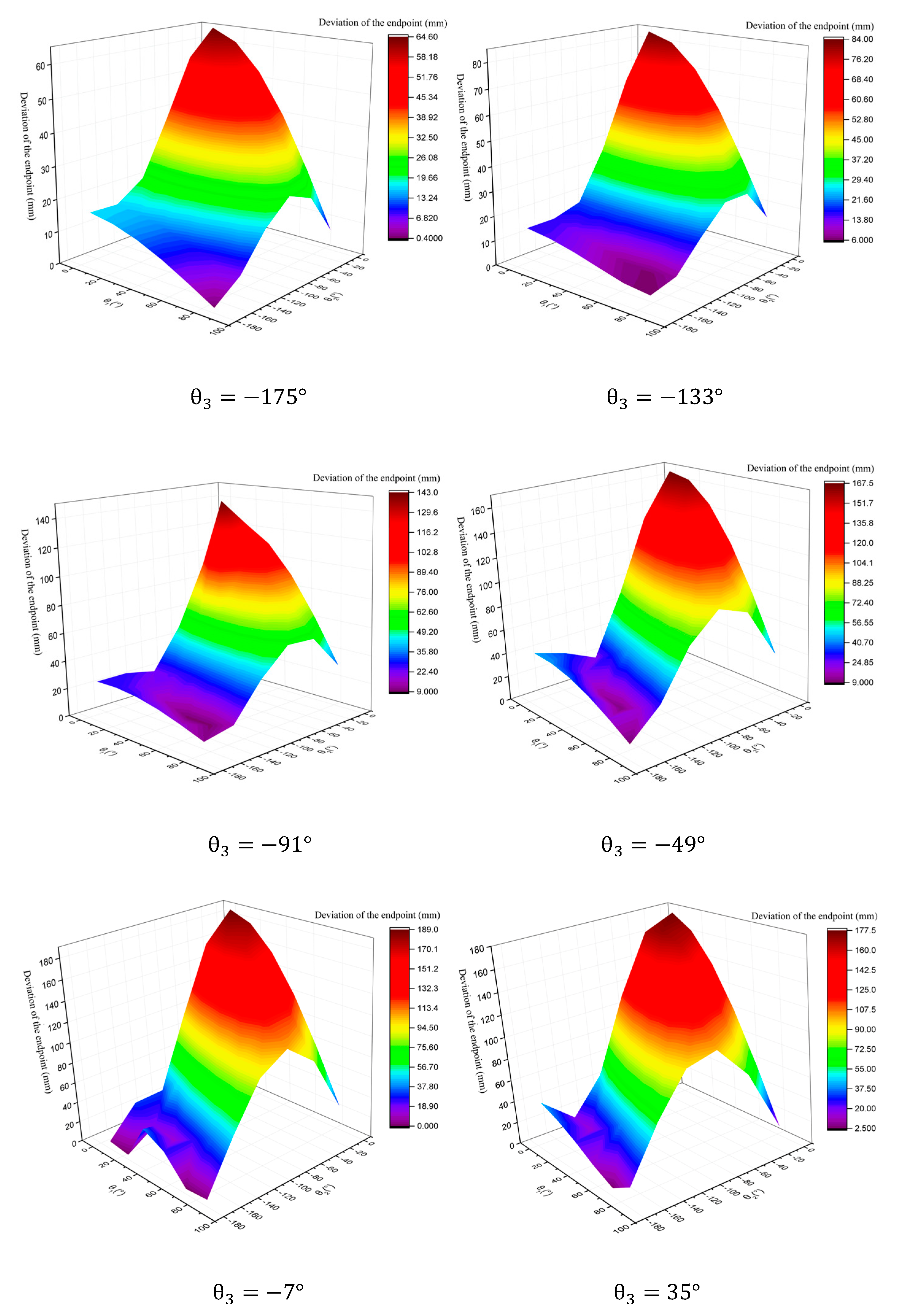
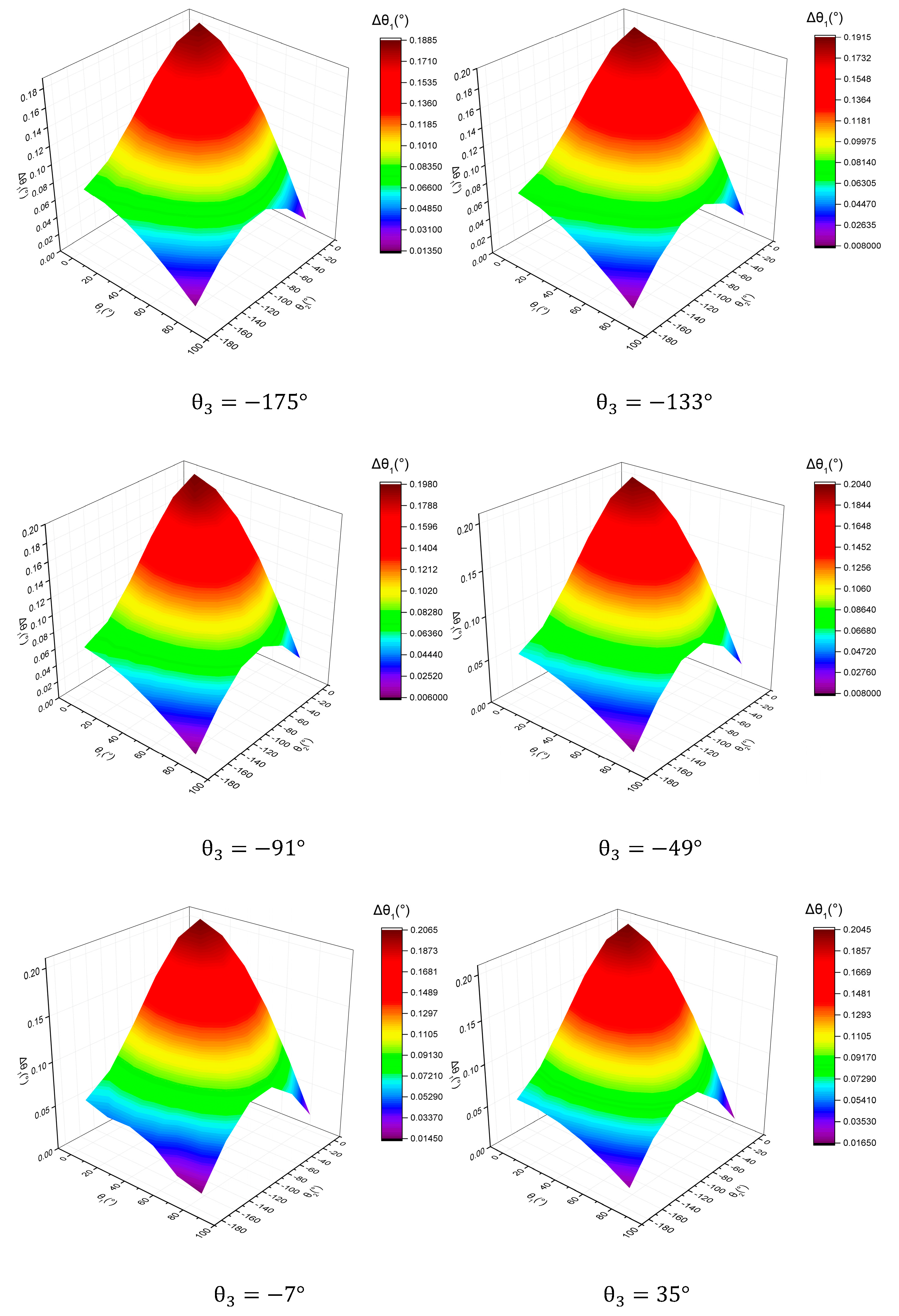
4.1.1. Parametric Simulation of Compensation Angle

Since ${\mathsf{\theta }}_0$ is the rotation angle of the rotation base, its influence on the deformation of the manipulator is little; take ${\mathsf{\theta }}_0=0$ in the simulation.

The range of joint angles is ${\mathsf{\theta }}_1\in \left[0,90\right];{\mathsf{\theta }}_2\in \left[-180,0\right];{\mathsf{\theta }}_3\in \left[-180,40\right],$ A total of 216 positions and orientations are simulated.

$${\left[\begin{array}{ccc}{\mathsf{\theta }}_1& {\mathsf{\theta }}_2& {\mathsf{\theta }}_3\end{array}\right]}^{\mathrm{T}}=\left[\begin{array}{cc}\begin{array}{ccc}\begin{array}{c}5\\ -175\\ -175\end{array}& \begin{array}{c}21\\ -141\\ -133\end{array}& \begin{array}{c}37\\ -107\\ -91\end{array}\end{array}& \begin{array}{ccc}\begin{array}{c}53\\ -73\\ -49\end{array}& \begin{array}{c}69\\ -39\\ -7\end{array}& \begin{array}{c}85\\ -5\\ 35\end{array}\end{array}\end{array}\right]$$

The relationship between the endpoint’s deviation of the mobile concrete pump manipulator and ${\mathsf{\theta }}_1{\mathsf{\theta }}_2 {\mathsf{\theta }}_3$ is obtained.

As shown in Figure 6, they are continuous three-dimensional relational surface diagrams between the endpoint’s deviation and ${\mathsf{\theta }}_1{\mathsf{\theta }}_2$ when ${\mathsf{\theta }}_3$ takes −175°, −133°, −91°, −49°, −7°, 35° respectively.

It can be seen that the larger the angle of the 2nd link unfolding, the larger the endpoint’s deviation will become, and the sharper the endpoint’s deviation will change when the 1st link’s corresponding action is performed. The position and orientation of the 3rd link has a certain influence on the total deformation of the end. The effect on the deviation when the 3rd link is in the approximate symmetrical orientation (such as 35° and −49°) is approximately the same.

The relationship between the 1st joint compensation angle and the and ${\mathsf{\theta }}_1{\mathsf{\theta }}_2 {\mathsf{\theta }}_3$ is obtained. As shown in Figure 7, they are continuous three-dimensional relational surface diagrams between the joint compensation angles $\Delta {\mathsf{\theta }}_1$ and ${\mathsf{\theta }}_1{\mathsf{\theta }}_2$ when ${\mathsf{\theta }}_3$ taking −175°, −133°, −91°, −49°, −7°, 35°.

It can be seen that the orientations of the 1st link and the 2nd link have a great influence on the compensation angle of the 1st joint and the orientation of the 3rd link has less influence. The compensation angle of the 1st joint reaches the maximum when the manipulator is fully extended.

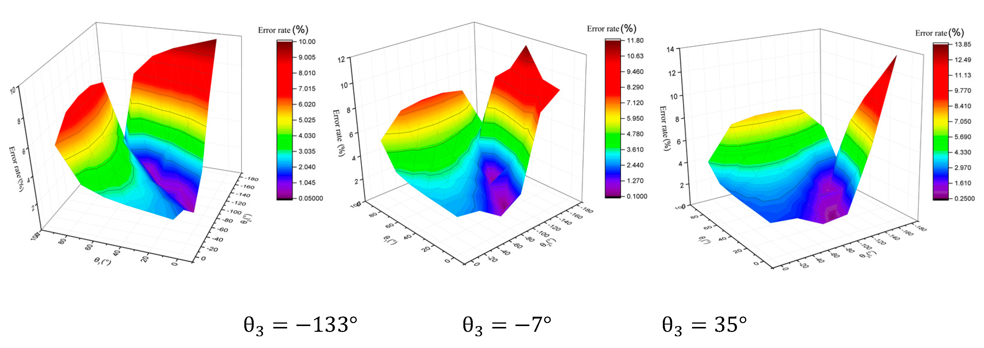
4.1.2. Parametric Simulation to Verify the Reliability of the Compensation Method

Considering the ratio of deflection and link length as the actual value of angle compensation, the accuracy of the compensation method can be verified by comparing the actual value of angle compensation and the angle compensation value obtained by this static deformation-compensation method. In this paper, the accuracy of the compensation method is measured by the error rate (actual value − calculated value)/(actual value).

The relationship between the compensation error rate of the 1st link and the joint angles is obtained. As shown in Figure 8, they are continuous three-dimensional relational surface diagrams between error rate and ${\mathsf{\theta }}_1 {\mathsf{\theta }}_2$ when ${\mathsf{\theta }}_3$ takes −133°, −7°, 35°.

It can be seen that when the manipulator is in various positions and orientations, the deformation compensation error rate is controlled within 14%, which verifies the reliability of the static deformation-compensation method based on the inclination sensor feedback. The orientations of the 1st and the 2nd links have a great influence on the deformation compensation error. It can be seen from the figure that the deformation compensation error is the smallest when the angles of the 1st and 2nd joints are in the middle of the value range, and there is a low error valley, which can be used as the research object in the future.

The main reason for the error is that using the secant slope approximates the tangent slope to obtain the inclination angle approximate value. In engineering practice, errors will be of two types: γi experimental determination and accuracy of the coefficient matrix (Equation (26)). In order to compensate the endpoint deviation of the concrete truck manipulator with a length of 24 m up to 200 mm, it is recommended that the accuracy of the inclination sensor is 0.01° to achieve better results.

4.2. Verification of Deformation Compensation Effect Based on ANSYS Workbench and MATLAB Co-Simulation

The six common orientations and six different loads of the 24m-3R mobile concrete pump manipulator were simulated by ANSYS Workbench and MATLAB co-simulation. The validity of the static deformation-compensation method was verified by comparing the theoretical endpoint position of the manipulator with the actual endpoint position (simulation result) after deformation compensation. The compensation error under different loads was obtained, and the universality of the compensation method to different loads was verified.

4.2.1. Verification of the Static Deformation-Compensation Method’s Validity

The six common orientations of the link were simulated by ANSYS Workbench and MATLAB co-simulation. ANSYS Workbench parametric simulation obtained the deformation value before and after deformation compensation and obtained the simulation values of inclination sensors; then the results were input to MATLAB, MATLAB according to the set joint angle and ANSYS Workbench input data real-time calculate the manipulator’s endpoint position. As shown in

Table 2. Deformation compensation effect of six common orientations.

$\mathbf{Orientation}(°)({\mathsf{\theta }}_{\mathbf{1}},{\mathsf{\theta }}_{\mathbf{2}},{\mathsf{\theta }}_{\mathbf{3}})$	Endpoint Deviation (mm)	Compensation Angle (°) $(\Delta {\mathsf{\theta }}_{\mathbf{1}},\Delta {\mathsf{\theta }}_{\mathbf{2}},\Delta {\mathsf{\theta }}_{\mathbf{3}})$	Endpoint Target Position (mm) $(\mathit{x},\mathit{z})$	Endpoint Position before Compensation (mm) $(\mathit{x},\mathit{z})$	Endpoint Position after Compensation (mm) $(\mathit{x},\mathit{z})$	Compensation Error (Residual Deviation) (mm) $(\mathit{x},\mathit{z})$
(5, −5, 35)	177.0635	(0.204, 0.181, 0.042)	(23042, 3834)	(23079.22, 3660.73)	(23055.25, 3784.12)	(13.25, 49.88)
(37, −5, 35)	140.1612	(0.163, 0.138, 0.022)	(17509, 15462)	(17606.04, 15360.49)	(17539.17, 15432.31)	(30.17, 29.69)
(53, −5, 35)	104.5001	(0.123, 0.100, 0.010)	(12569, 19689)	(12659.12, 19635.76)	(12596.90, 19673.30)	(27.90, 15.70)
(53, −73, −49)	105.5360	(0.147, 0.146, 0.015)	(15858, 1629)	(15814.44, 1533.23)	(15829.77, 1596.88)	(28.23, 32.12)
(69, −73, −49)	101.2360	(0.120, 0.171, 0.027)	(14794, 5937)	(14773.62, 5837.99)	(14777.04, 5901.81)	(16.96, 35.19)
(85, −73, −49)	89.38721	(0.083, 0.183, 0.037)	(12585, 9785)	(12585.90, 9695.61)	(12578.28, 9753.63)	(6.72, 31.37)

, the deformation compensation effects of six common orientations were obtained.

The deformation compensation error of the mobile concrete pump manipulator in different orientations under no-load operation can be controlled within 50 mm. Compared with the endpoint deviation of 177 mm before compensation, the effect of deformation compensation is obvious. The validity of this method was verified.

4.2.2. Verification of the Static Deformation-Compensation Method’s Universality for Different Loads

Six different loads of the 24m-3R mobile concrete pump manipulator in a certain orientation were simulated by ANSYS Workbench and MATLAB co-simulation. In engineering practice, in order to make the concrete pumpable, the concrete in the pipeline is a fluid liquid. In the simulation analysis of concrete pumping, there is a consensus on the treatment of the liquid concrete in the pipeline. In the analysis and calculation, the rigidity of the liquid concrete is not considered, and it is directly applied to the pipeline arch rib as an external load. This method is supported by many engineering application backgrounds, and the calculated results are consistent with the corresponding measured results. Considering the concrete load has the same uniformity as gravity when verifying the static deformation-compensation method is universal for different loads, the equivalent density of the manipulator is changed in the parametric modeling. The simulation results are shown in

Table 3. Deformation compensation effect of different equivalent density.

Equivalent Density (kg/m3)	Endpoint Deviation (mm)	Compensation Angle (°) $(\Delta {\mathsf{\theta }}_1,\Delta {\mathsf{\theta }}_2,\Delta {\mathsf{\theta }}_3)$	Endpoint Target Position (mm) $(\mathit{x},\mathit{z})$	Endpoint Position before Compensation (mm) $(\mathit{x},\mathit{z})$	Endpoint Position after Compensation (mm) $(\mathit{x},\mathit{z})$	Compensation Error (Residual Deviation) (mm) $(\mathit{x},\mathit{z})$
7000	177.0635	(0.204, 0.181, 0.042)	(23042, 3834)	(23079.22, 3660.73)	(23055.25, 3783.82)	(13.25, 50.18)
8272	209.2331	(0.241, 0.214, 0.049)	(23042, 3834)	(23085.98, 3629.25)	(23058.42, 3774.71)	(16.42, 59.29)
11116	281.1570	(0.324, 0.288, 0.066)	(23042, 3834)	(23101.10, 3558.87)	(23063.69, 3754.57)	(21.69, 79.43)
13959	353.0808	(0.407, 0.361, 0.083)	(23042, 3834)	(23116.21, 3488.48)	(23070.30, 3734.47)	(28.30, 99.53)
16803	425.0046	(0.490, 0.435, 0.100)	(23042, 3834)	(23131.33, 3418.10)	(23076.25, 3714.50)	(34.25, 119.50)
19646	496.9285	(0.573, 0.509, 0.117)	(23042, 3834)	(23146.45, 3347.72)	(23082.54, 3694.66)	(40.54, 139.34)

, and the selected orientation was (5, −5, 35).

By changing the equivalent density, the deformation compensation effect of the manipulator under different materials and loads was obtained.

The compensation error increased with the increase of the equivalent density, but the endpoint deviations were all reduced to about 20% of the original endpoint deviations after the compensation. The static deformation-compensation method’s universality for different loads was verified.

5. Conclusions and Future Work

In this paper, we propose a static deformation-compensation method based on inclination sensor feedback for large-scale manipulators with hydraulic actuation like mobile concrete pump manipulators, maritime crane systems, and so on to reduce the deviation of the endpoint. Compared with the finite element method, this method does not need to consider many boundary conditions that are uncertain for flexible manipulators in most situations. It has appropriate accuracy and is universal for large-scale manipulators of different sizes and working under different loads.

Based on a 24m-3R mobile concrete pump manipulator, the parametric simulation based on ANSYS is carried out. The relationship between the endpoint’s deviation of the mobile concrete pump manipulator and ${\mathsf{\theta }}_1{\mathsf{\theta }}_2 {\mathsf{\theta }}_3$ and the relationship between the compensation error rate of the 1st link and the joint angles are obtained. When the manipulator is in various positions and orientations, the deformation compensation error rate is controlled within 14%. The reliability of the static deformation-compensation method is verified, and the error of this method is analyzed.

Based on the ANSYS and MATLAB co-simulation, we compared the theoretical endpoint position with the actual endpoint position after deformation compensation. The deformation compensation error of the mobile concrete pump manipulator in different orientations under no-load operation can be controlled within 50 mm. Compared with the endpoint deviation of 177 mm before compensation, the effect of deformation compensation is obvious. The validity of this method is verified.

Besides, the compensation error under different loads is obtained. The compensation error increases with the increase of the equivalent density, but the endpoint deviations are all reduced to about 20% of the original endpoint deviations after the compensation. The universality of the compensation method for different loads is verified.

In the future, experiments based on this method will be performed to verify the feasibility of the method and to evaluate the deformation-compensation effectiveness of this method in practical application.

References

1. Dwivedy, S.K.; Eberhard, P. Dynamic analysis of flexible manipulators, a literature review. Mech. Mach. Theory 2007, 41, 749–777. [Google Scholar] [CrossRef]
2. Book, W.J.; Majette, M. Controller design for flexible distributed parameter mechanical arm via combined state-space and frequency domain techniques. Trans. ASME: J. Dyn. Syst. Meas. Contr. 1983, 105, 245–254. [Google Scholar] [CrossRef]
3. Azad, A.K.M. Analysis and Design of Control Mechanisms for Flexible Manipulator Systems. Ph.D. Thesis, Department of Automatic Control and Systems Engineering, The University of Sheffield, Sheffield, UK, 1994. [Google Scholar]
4. Poerwanto, H. Dynamic Simulation and Control of Flexible Manipulator Systems. Ph.D. Thesis, Department of Automatic Control and Systems Engineering, The University of Sheffield, Sheffield, UK, 1998. [Google Scholar]
5. Hartmut, B. Mechydronic for Boom Control on Truck Mounted Concrete Pumps. Tech. Symp. Constr. Equip. Technol. 2003, 1, 12. [Google Scholar]
6. Henikl, J.; Kemmetmüller, W.; Meurer, T.; Elsevier, A.K. Infinite-dimensional decentralized damping control of large-scale manipulators with hydraulic actuation. Automatica 2016, 63, 101–115. [Google Scholar] [CrossRef]
7. Liu, J.; Dai, L.; Zhao, L.; Cai, J.; Zhang, W. Flexible multi-body dynamics modeling and simulation of concrete pump truck boom. J. Mech. Eng. 2007, 1, 131–135. [Google Scholar] [CrossRef]
8. Keating, S.J.; Leland, J.C.; Cai, L. Toward site-specific and self-sufficient robotic fabrication on architectural scales. Sci. Robot. 2017, 2, eaam8986. [Google Scholar] [CrossRef]
9. Cheng, M.; Zhang, J.; Xu, B.; Ding, R. An Electrohydraulic Load Sensing System based on flow/pressure switched control for mobile machinery. ISA Trans. 2019. [Google Scholar] [CrossRef]
10. Bradley, D.A.; Seward, D.W. Developing real-time autonomous excavation-the LUCIE story. In Proceedings of the 34th IEEE Conference on Decision and Control, New Orleans, LA, USA, 13–15 December 1995; pp. 3028–3033. [Google Scholar]
11. Bradley, D.; Seward, D. The development, control and operation of an autonomous robotic excavator. J. Intell. Robot. Syst. 1998, 21, 73–97. [Google Scholar] [CrossRef]
12. Nguyen, Q.H.; Ha, Q.P.; Rye, D.C.; Durrant-Whyte, H.F. Force/position tracking for electro-hydraulic systems of a robotic excavator. In Proceedings of the 39th IEEE Conference on Decision and control, Sydney, NSW, Australia, 12–15 December 2000; pp. 5224–5229. [Google Scholar]
13. Ha, Q.P.; Nguyen, Q.H.; Rye, D.C.; Durrant-Whyte, H.F. Fuzzy sliding-mode controllers with applications. Ieee Trans. Ind. Electron. 2001, 48, 38–46. [Google Scholar] [CrossRef]
14. Lee, S.U.; Chang, P.H. Control of a heavy-duty robotic excavator using time delay control with integral sliding surface. Control Eng. Pract. 2002, 10, 697–711. [Google Scholar] [CrossRef]
15. Chang, P.H.; Lee, S.J. A straight-line motion tracking control of hydraulic excavator system. Mechatronics 2002, 12, 119–138. [Google Scholar] [CrossRef]
16. Budny, E.; Chlosta, M.; Gutkowski, W. Load-independent control of a hydraulic excavator. Autom. Constr. 2003, 12, 245–254. [Google Scholar] [CrossRef]
17. Araya, H.; Makoto, K.; Kinugawa, H.; Tatsuo, A. Level luffing control system for crawler cranes. Autom. Constr. 2004, 13, 689–697. [Google Scholar] [CrossRef]
18. Guo, L.; Zhang, G.; Li, J. Kinematics analysis and trajectory planning control modeling and simulation of concrete pump truck. Constr. Mach. 2000, 4, 29–32. [Google Scholar]
19. Guo, L.; Zhao, M.; Zhang, G.; Huang, Y. Automatic pumping and process simulation of concrete pump truck cloth mechanism. J. Northeast. Univ. (Nat. Sci. Ed.) 2000, 21, 617–619. [Google Scholar]
20. Zhipeng, Y. Research on the end Track Control of the Concrete Pump Truck Boom; Wuhan University of Science and Technology: Wuhan, China, 2018. [Google Scholar]
21. Bremer, H. Elastic Multibody Dynamics: A Direct Ritz Approach; Springer: Dordrecht, The Netherlands, 2008. [Google Scholar]
22. Henikl, J.; Kemmetmüller, W.; Bader, M.; Kugi, A. Modeling, simulation and identification of a mobile concrete pump. Math. Comput. Model. Dyn. Syst. 2015, 21, 180–201. [Google Scholar] [CrossRef]
23. Henikl, J.; Kemmetmüller, W.; Kugi, A. Modeling and control of a mobile concrete pump. In Proceedings of the 6th IFAC Symposium of Mechatronic Systems, Hangzhou, China, 10–12 April 2013; pp. 91–98. [Google Scholar]
24. Lambeck, S.; Sawodny, O.; Arnold, E. Trajectory tracking control for a new generation of fire rescue turntable ladders. In Proceedings of the 2nd IEEE Conference on Robotics, Automation and Mechatronics, Orlando, FL, USA, 15–19 May 2006; pp. 847–852. [Google Scholar]
25. Zimmert, N.; Pertsch, A.; Sawodny, O. 2-DOF control of a fire-rescue turntable ladder. IEEE Trans. Control Syst. Technol. 2012, 20, 438–452. [Google Scholar] [CrossRef]
26. Book, W.J. Modeling, design, and control of flexible manipulator arms: A tutorial review. In Proceedings of the IEEE Conference on Decision and Control, Honolulu, HI, USA, 5–7 December 1990; pp. 500–506. [Google Scholar]
27. Rahimi, H.N.; Nazemizadeh, M. Dynamic analysis and intelligent control techniques for flexible manipulators: A review. Adv. Robot. 2013, 28, 63–76. [Google Scholar] [CrossRef]
28. Kiang, T.; Spowage, A.; Yoong, C.K. Review of control and sensor system of flexible manipulator. J. Intell. Robot. Syst. 2015, 77, 187–213. [Google Scholar] [CrossRef]
29. Theodore, R.J.; Ghosal, A. Comparison of the assumed modes and finite element models for flexible multi-link manipulators. Int. J. Robot. Res. 1995, 14, 91–111. [Google Scholar] [CrossRef] [Green Version]
30. Huang, D.; Chen, L. Partitioned neural network control and fuzzy vibration control for free-floating space flexible manipulator. Eng. Mech. 2012, 37. [Google Scholar] [CrossRef]
31. Subudhi, B.; Morris, A.S. Dynamic modelling, simulation and control of a manipulator with flexible links and joints. Rob. Auton. Syst. 2002, 41, 257–270. [Google Scholar] [CrossRef]
32. Usoro, P.B.; Nadira, R.; Mahil, S.S. A finite element/lagrangian approach to modeling light weight flexible manipulators. ASME J. Dyn. Syst. Meas. Contr. 1986, 108, 198–205. [Google Scholar] [CrossRef]
33. Zienkiewicz, O.C.; Taylor, R.L.; Zhu, J.Z. The Finite Element Method, Its Basis and Fundamentals; Butterworth-Heinemann: Oxford, UK, 2005. [Google Scholar]
34. Geradin, M.; Cardona, A. Kinematics and dynamics of rigid and flexible mechanisms using finite elements and quaternion algebra. Comput. Mech. 1988, 4, 115–135. [Google Scholar] [CrossRef]
35. Bayo, E. A finite-element approach to control the end point motion of a single link flexible robot. Rob. Syst. 1987, 4, 63–75. [Google Scholar] [CrossRef]
36. Jonker, B. A finite element dynamic analysis of flexible spatial mechanisms with flexible links. Comput. Methods Appl. Mech. Eng. 1989, 76, 17–40. [Google Scholar] [CrossRef]
37. Jonker, B. A finite element dynamic analysis of flexible manipulators. Int. J. Rob. Res. 1990, 9, 59–74. [Google Scholar] [CrossRef]
38. Hastings, G.G.; Book, J.W. Verification of a linear dynamic model for flexible robotic manipulators. In Proceedings of the IEEE International Conference on Robotics and Automation, Francisco, CA, USA, 7–10 April 1986; pp. 1024–1029. [Google Scholar]
39. Kim, J.S.; Uchiyama, M. Vibration mechanism of constrained spatial flexible manipulators. JSME Ser. C 2003, 46, 123–128. [Google Scholar] [CrossRef]
40. Feliu, V.; Rattan, K.S.; Brown, H.B. Modeling and control of single-link flexible arms with lumped masses. ASME J.Dyn. Syst. Meas. Contr. 1992, 114, 59–69. [Google Scholar] [CrossRef]
41. Khalil, W.; Gautier, M. Modeling of mechanical systems with lumped elasticity. Proc. IEEE Int. Conf. Rob. Autom. 2000, 4, 3964–3969. [Google Scholar]
42. Zhu, G.; Ge, S.S.; Lee, T.H. Simulation studies of tip tracking control of a single-link flexible robot based on a lumped model. Robotica 1999, 17, 71–78. [Google Scholar] [CrossRef]
43. Raboud, D.W.; Lipsett, A.W.; Faulkner, M.G.; Diep, J. Stability evaluation of very flexible cantilever beams. Int. J.Nonlinear Mech. 2001, 36, 1109–1122. [Google Scholar] [CrossRef]
44. Lee, S.J.; Chung, I.S.; Bae, S.Y. Structural design and analysis of CFRP boom for concrete pump truck. Mod. Phys. Lett. B 2019, 33, 787–792. [Google Scholar] [CrossRef]
45. Yuan, Q.H.; Lew, J.; Piyabongkarn, D. Motion control of an aerial work platform. In Proceedings of the 2009 American control conference, AACC 2009, Hyatt Regency Riverfront, St. Louis, MO, USA, 10–12 June 2009; pp. 2873–2878. [Google Scholar]
46. Xia, J.; Gang, G.; Xin, Z. Research on deformation compensation and trajectory control technology of concrete boom. Constr. Mach. 2016, 5, 70–76. [Google Scholar]
47. Xin, Z.; Liang, W.; Jiaqian, W.; Shiyang, H. Research on trajectory control technology of concrete pump truck based on vehicle deformation compensation. J. Mech. Eng. 2015, 13, 492–496. [Google Scholar]
48. Wang, X. Research on Trajectory Control Technology of Concerte Pump Arm Frame based on Arm Frame Denaturalization Compensation. Master’s Thesis, Qingdao University of Science and Technology, Qingdao, China, 2018. [Google Scholar]
49. Pan, D.; Xing, J.; Wang, B. Static Analysis and Dynamic Simulation of Concrete Pump Truck Boom. J. Chongqing Univ. Technol. (Nat. Sci.) 2018, 32, 86–91, 123. [Google Scholar]
Figure 1. Structure diagram of the mobile concrete pump manipulator. 1. Rotation base; 2. 1st joint; 3. 1st link; 4. 2nd joint; 5. 2nd link; 6. 3rd joint; 7. 3rd link; 8. End outlet; 9. Concrete discharge hose.
Processes 08 00081 g001
Figure 2. Denavit–Hartenberg (D–H) coordinate system of the mobile concrete pump manipulator.
Processes 08 00081 g002
Figure 3. The basic principle of joint angle independent compensation.
Processes 08 00081 g003
Figure 4. Schematic diagram of installation positions of inclination sensors.
Processes 08 00081 g004
Figure 5. The tangent angle solution method.
Processes 08 00081 g005
Figure 6. Relationship of endpoint deviation and each joint angle.
Processes 08 00081 g006
Figure 7. Relationship of compensation angle of the 1st joint angle and each joint angle.
Processes 08 00081 g007
Figure 8. Relationship of compensation error of the 1st joint angle and each joint angle.
Processes 08 00081 g008