Review

Modeling and Exploiting Microbial Temperature Response

Institute of Food Science and Biotechnology, Department of Bioprocess Engineering (150k), University of Hohenheim, Fruwirthstr. 12, 70599 Stuttgart, Germany
*
Author to whom correspondence should be addressed.
Processes 2020, 8(1), 121; https://doi.org/10.3390/pr8010121
Submission received: 15 December 2019 / Revised: 5 January 2020 / Accepted: 14 January 2020 / Published: 17 January 2020
(This article belongs to the Special Issue Bioprocess Monitoring and Control)

Abstract

:
Temperature is an important parameter in bioprocesses, influencing the structure and functionality of almost every biomolecule, as well as affecting metabolic reaction rates. In industrial biotechnology, the temperature is usually tightly controlled at an optimum value. Smart variation of the temperature to optimize the performance of a bioprocess brings about multiple complex and interconnected metabolic changes and is so far only rarely applied. Mathematical descriptions and models facilitate a reduction in complexity, as well as an understanding, of these interconnections. Starting in the 19th century with the “primal” temperature model of Svante Arrhenius, a variety of models have evolved over time to describe growth and enzymatic reaction rates as functions of temperature. Data-driven empirical approaches, as well as complex mechanistic models based on thermodynamic knowledge of biomolecular behavior at different temperatures, have been developed. Even though underlying biological mechanisms and mathematical models have been well-described, temperature as a control variable is only scarcely applied in bioprocess engineering, and as a conclusion, an exploitation strategy merging both in context has not yet been established. In this review, the most important models for physiological, biochemical, and physical properties governed by temperature are presented and discussed, along with application perspectives. As such, this review provides a toolset for future exploitation perspectives of temperature in bioprocess engineering.

1. Introduction

Predetermined by the applied system, bioprocesses are generally very sensitive to most changes in environmental conditions. It is for this reason that conditions such as temperature, pO2, or pH are generally tightly controlled. In most cases, even small deviations from optimum values may lead to a significant reduction in the overall productivity and reproducibility of the process. Therefore, special consideration must be given to control tasks, which are typically defined by maintaining process variables within a narrow optimum [1]. In contrast to artificial laboratory conditions, microorganisms are usually exposed to a changing environment, with changes in pH, nutrient availability, competitors, and elevated or decreased temperature, etc. A crucial environmental factor for microorganisms is temperature. It affects the folding, structure, and stability of almost every biomolecule, as well as the metabolic reaction rate. Detection of temperature changes and subsequent adaptation of the metabolism are essential for microbial survival, such as by pathogens sensing intrusion into a host. Organisms can sense temperature shifts indirectly or by specialized sensing systems that evolved to detect changes in temperature in order to respond with adapted gene expression. This was extensively reviewed by Klinkert and Narberhaus [2]. Indirect temperature sensing is possible via the accumulation of aggregated proteins after a heat shock and via stalled ribosomes after a cold shock. Molecular thermosensors may consist of DNA, RNA, proteins, or lipids. DNA topology changes, e.g., supercoiling caused by heat stress, stable RNA structures preventing translation at sub-optimal temperatures, temperature-responsive regulatory proteins, and alterations in lipid membrane stability with respective to fluidity are just a few examples for direct temperature sensing. Temperature plays an essential role and has a crucial effect on biological processes. Targeted temperature adjustments for triggering a desired response may also be exploited for biotechnological applications. Noll et al. published an example for a thermosensitive structure to direct the carbon flow of a substrate into a product rather than into biomass, by exploiting an RNA thermometer to optimize the heterologous production of rhamnolipid biosurfactants [3].
Alterations in temperature lead to multiple, often complex, interconnected metabolic changes. Models describing a biological process as a function of temperature are therefore indispensable to reducing complexity and facilitating understanding of those interconnections. Mathematical descriptions of how (bio-)chemical reactions respond to high or low temperatures emerged as early as in the 1900s with the “primal” temperature model of Arrhenius [4]. He investigated the reaction kinetics for sugar cane inversion by acids, depending on temperature. Popularized by Arrhenius, a variety of temperature models evolved over time, as shown in Figure 1. These models range from data-driven empirical approaches to complex mechanistic models that are based on thermodynamic knowledge of biomolecular behavior at different temperatures. Models are readily available to be used as a tool for process control and design. An overview of the current state of thermo-modeling is crucial to reasonably selecting a suitable model for the bioprocess to be monitored or optimized. The aim of this review is to provide an overview of available temperature models to facilitate understanding of model intention and reasonable selection for application. So far, only a few applications for temperature in (industrial) process design, monitoring, and control have been described. Applied model approaches are usually based on fuzzy logic or artificial neural networks and do not harvest the full potential of deterministic approaches. There are a few examples for applied model-assisted temperature control strategies in industrial biotechnology. These include heat balancing for an estimation of metabolic activity to improve batch-to-batch reproducibility by applying a process control module which uses the difference between the culture temperature and temperature of a coolant to predict oxygen mass transfer rates and kLa values [5,6,7]. Furthermore, deterministic process models can be used to describe a biological process as a function of a physical condition, like the temperature. They may be used in the food sector to estimate product shelf life, determining critical control points of a process, or to maximize productivities and ensure safe distribution chains [8]. These examples highlight a potential for temperature and deterministic models in process design. An approach for experimental design to optimize processes depending on multiple parameters is the Response Surface Method (RSM): “RSM is a collection of statistical techniques used for studying the relationships between measured responses and independent input variables” [9]. This method may be used for optimization purposes in experimental design in the shape of a metamodel. It connects the response of an objective function to input variables and determines its relations, for example, by the means of first- or second-order polynomial equations. The Matlab software package from The Mathworks, Inc. (Natick, MA, USA) [10] or the Minitab statistic software (GMSL s.r.l., UK) [11] may be used to conduct an RSM analysis. In bioprocesses, usually very few process variables are available online that continuously display a process course. Furthermore, arguably the only control variable to direct a bioprocess towards a desired outcome is, in most cases, the addition of fresh media. Other variables like pH, temperature, or pO2 are typically controlled at a constant value. Therefore, investigating and exploiting novel potentially available monitoring and control variables like temperature is a reasonable strategy to extend existing toolsets of bioprocess monitoring and control. Even though several systems inducible by temperature have been discovered and made available to biotechnologists in the last decades, only a few have been exploited for practical purposes, such as for process design or optimization [12]. For monitoring and control purposes, calorimetric approaches have been presented [5,6,13,14]. For control purposes, temperature may be used to directly address biological traits like RNA-thermometers to provoke a desired response, as previously evaluated [3]. Furthermore, indirect metabolic effects may be exploited, like elevated metabolic rates at high temperatures or the correct folding of proteins at low temperatures. Even though knowledge on microbial temperature responses and adaptation, along with descriptions developed by mathematical means, is available, its potential for applied industrial bioprocesses has not been sufficiently exploited. This review provides an overview on available thermo-models with the potential to develop model-assisted or model-derived process control strategies using temperature as a crucial parameter.

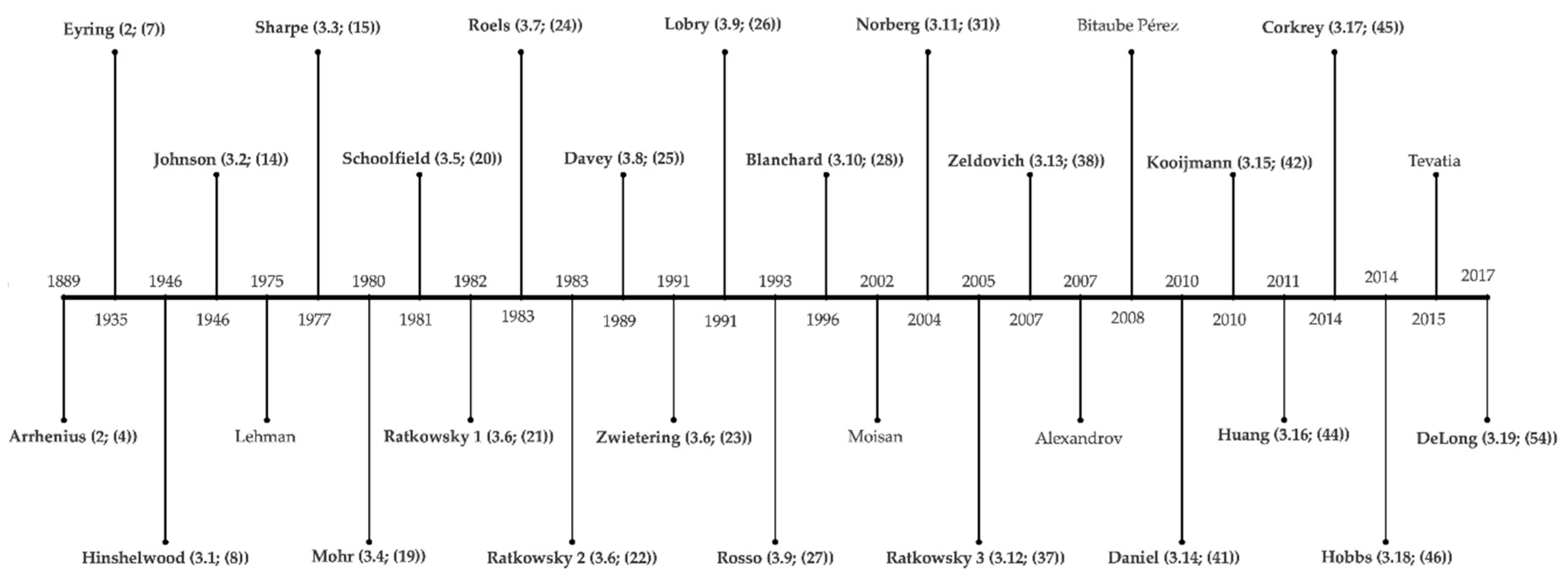
2. History of Temperature Modeling—17th–20th Century

As early as the 17th century, there were theories on temperature being a form of particle movement. The kinetic theory of gases, with its origins in the 18th century, first specifically associated translational motions of molecules with heat and not with their vibrational or rotational motions [15]. Daniel Bernoulli was the pioneer of the kinetic theory of gases. He hypothesized that gases consist of a finite number of small spherical particles, which move through space along a straight line with high velocities. He assumed that heat increases the particle speed (v) and demonstrated that air pressure correlates with v2. Air temperature can therefore be measured by this pressure at a constant density, making temperature proportional to v2 [16,17]. The kinetic energies of the molecules are correlated with the ideal gas law of Equation (1), whose history began with the French engineer Émile Clapeyron in 1834 [18,19]. In the following, only SI units are used. Parameters with non-SI units, used by cited authors, were converted into SI units.
p   ·   V   =   n   ·   R   ·   T
where p is the pressure, Pa; V is the volume, m3; n is the amount of substance, mol; R is the universal gas constant ~8.314, J mol−1 K−1; and T is the absolute temperature, K. The Dutch chemist and first Nobel Prize laureate J. H. Van’t Hoff observed that the chemical reaction rate doubles or triples when the temperature is increased by 10 K, which he expressed with the following equation:
Q 10 =   ( k 2 k 1 ) 10   T 2 T 1
This “rule of thumb” for chemical kinetics allows estimations for various phenomena in chemistry, biochemistry, and ecology. He furthermore described the change in the equilibrium constant K of a chemical reaction with respect to the change in temperature at constant pressure with the Van’t Hoff Equation (3):
d d T ln K eq =   Δ H R   · T 2
where K is the dimensionless equilibrium constant; ΔH is the standard enthalpy change, J mol−1; R is the universal gas constant ~8.314, J mol−1 K−1; and T is the absolute temperature, K. Van’t Hoff’s student and the father of temperature models Svante Arrhenius continued the work of his teacher on the description of temperature-dependent specific reaction rate constants in chemical reactions with his essay “On the Reaction Velocity of the Inversion of Cane Sugars by Acids” [4]. Arrhenius observed that the reaction velocity of chemical reactions increased between 10% and 15% for each degree of rising temperature and postulated a semi-empirical model based on the Van’t Hoff equation, which is shown in its integrated form in Equation (4).
k   =   A · e E a R · T
where k is the rate constant, s−1, for a first-order rate constant; A is called a pre-exponential frequency or collision factor, s−1, for a first-order rate constant; Ea is an empirical parameter, the (Arrhenius) activation energy, J mol−1, characterizing the exponential temperature dependence of k; R is the universal gas constant ~8.314, J mol−1 K−1; and T is the absolute temperature, K. In 1935, Henry Eyring formulated a statistical mechanistic equation following the transition state theory (former activated-complex theory) that assumed a transition state complex ( T C ) and a quasi-type equilibrium between educts (e1; e2), the transition state, and the product (P) [20,21]. The model has a similar way of describing the variance of the rate of a chemical reaction with temperature as the equation of Arrhenius. Therefore, it underlined Arrhenius’ previous observations and assumptions with a mechanistic approach.
e 1 + e 2 k 1 k 2 T C k 3 P
According to the transition state theory, the rate constant can be described as follows:
k ( T ) =   k B · T h · K
where kB is the Boltzmann constant ~1.381 ⋅10−23, J K−1; T is the absolute temperature, K; h is the Planck’s constant ~6.626⋅10−34, J s−1; and K is the dimensionless equilibrium constant. A different way to express the rate constant is by replacing the equilibrium constant with a term containing the standard molar changes of entropy and enthalpy:
k ( T ) =   k B · T h · e Δ S ° / R · e Δ H ° / ( R · T )
where the entropy and enthalpy of activation are the standard molar change of entropy Δ S ° , J K−1 mol−1, when reactants form the transition state (activated) complex and standard molar change of enthalpy Δ H ° , respectively, J mol−1. R is the universal gas constant ~8.314, J mol−1 K−1. The (Arrhenius) activation energy (Ea) and enthalpy of activation are not the same, but approximately equal, as they are convertible, depending on the molecularity [22].

2.1. Temperature in Biological Systems—The History Began with Arrhenius

Microbiologists have noticed a major effect of temperature on the growth rate of microbial populations and described this effect with the Arrhenius equation by simply replacing the rate constant k in Equation (4) with the growth rate (µ), meaning the reciprocal of the generation time. The so-called Arrhenius plot, where ln(µ) is plotted against the reciprocal temperature, was used in the past and is still applied today to describe a relation between the temperature and growth of different bacteria and molds [23,24,25,26]. From this plot, Arrhenius parameters can easily be derived. Their plots show a good fit for lower temperatures. The Arrhenius model does not represent cell death, so a decrease of the growth curve at non-physiological temperatures. The lack of fit of the Arrhenius model for some temperature-dependent biological processes gave rise to the development of improved models describing growth as a function of temperature. Most of these models are based on Arrhenius’ parental model and evolved over time.

2.2. Biological Mechanisms Involved in Temperature Responses

Microorganisms have developed molecular traits to respond to changing environmental temperatures. These traits have been extensively reviewed [2,27,28]. The principles of microbial thermo responses range from changing DNA topology, e.g., supercoiling caused by heat stress, stalled ribosomes, or stable RNA preventing translation during cold stress to proper folding of proteins, working optima of enzymes, or lipid membrane stability and fluidity. Biomolecules are generally thermos-sensitive. Therefore, various options for direct molecular thermosensing are possible. Molecular thermosensors may consist of DNA, RNA, proteins, or lipids [2]. The accessibility of DNA for the transcriptional machinery is crucial for transferring genetic information via RNA into a protein and is influenced by DNA topology [29]. DNA supercoiling, and thus accessibility, is altered in response to a shifting temperature, as has been reported for the plasmic DNA of meso- and thermophiles [30]. Mesophiles have negatively supercoiled plasmic DNA and hyperthermophilic archaea with a growth optimum ≥80 °C have relaxed or positively supercoiled plasmic DNA [30,31,32]. Proteins such as the histone-like structuring proteins (H-NS) work as temperature-dependent regulators, governing >200 temperature-regulated genes in Salmonella sp. and more than two third of E. coli K-12 temperature-regulated genes, respectively [33,34]. The inhibition of gene expression by H-NS is caused by trapping RNA polymerase and mediating DNA looping, thereby disturbing the progression of RNA polymerase [35,36,37,38]. Temperature-dependent gene expression is also influenced on the RNA level, where RNA can form inhibitory loop structures called RNA-thermometers (RNAT). Here, base pairing blocks the Shine-Dalgarno-sequence (SD) and AUG start codons, inhibiting ribosomal binding and translation initiation. By raising the temperature to a threshold (melting temperature), the hairpin structure opens and permits the access of ribosomes to the translation initiation site [2,39]. The secondary structure and thereby functionality of RNAT is characterized by canonical or non-canonical base paring, internal loops or mismatches, and the total number of loop structures. Based on these characteristics, RNA thermometers may be subdivided into three categories: (i) ROSE-like RNATs (repression of heat shock gene expression), (ii) FourU RNATs, and (iii) additional types of RNATs [40]. Most RNATs have been identified in the 5′-UTR of mRNA. The ROSE-like RNAT family is probably the most abundant temperature-sensing mRNA structure. ROSE-like RNATs usually control the repression of heat shock gene expression, but have also been reported to control expression of the rhamnosyl transferase, which is associated with Pseudomonas aeruginosa virulence [41]. ROSE-RNATs are located in the 5′UTR, are between 60 and 100 nt in length, and consist of 2–4 loop structures [41,42,43]. The majority of described RNATs of the second family, the FourU RNATs, govern the gene expression of virulence genes, and only two FourU RNAT’s are known to control heat shock protein formation. FourU RNATs contain a sequence of four Uridines that occlude the SD sequence by canonical A-U and/or non-canonical G-U base pairing [40]. The virulence gene lcrF (virF) of Yersina pestis and the agsA small heat shock gene of Salmonella enterica were among the first genes described to be governed by a FourU RNAT [44]. Furthermore, attempts have been made to design synthetic RNATs with tailor-made characteristics to differ in up to 10-fold sensitivity- and around 3-fold threshold changes compared to a starting thermometer sequence [45]. On the protein level, global repressors, sensor kinases, methyl-accepting chemotaxis proteins (MCPs), M-like proteins, chaperones, and proteases are involved in microbial temperature responses [2]. The global transcriptional repressor CtsR has been termed a “protein thermosensor”, and liberates DNA upon an up-shift in temperature connected to the expression of heat shock proteins. Due to a glycine-rich loop structure, CtsR exhibits intrinsic heat-sensing characteristics [46]. MCPs function as transmembrane receptors and consist of a periplasmic ligand-binding domain and a signaling domain in the cytosol that can interact with cytosolic sensor kinases [47]. The Tar MCP, for example, is convertible from a heat to a cold sensor in the presence of aspartate and consequent methylation at up to four sites [48]. The surface M and M-like proteins of the human pathogens group A streptococci bind to a variety of human plasma proteins in a temperature-dependent manner. The affinity of the M-like coild-coil protein Arp4 to IgA, is high at 10 and 20 °C, but low at 37 °C, due to a conformational change of Arp4 and consequent loss of the coild-coil conformation and binding activity [49]. The diverse class of small heat shock proteins (sHsp) can act as molecular chaperones upon heat shock. They are temperature sensors with different molecular mechanisms. For example, the sHsp Hsp26 of Saccharomyces cerevisiae consists of 24 subunits and changes its affinity state towards unfolded proteins at high temperatures by undergoing a conformational change [50,51].

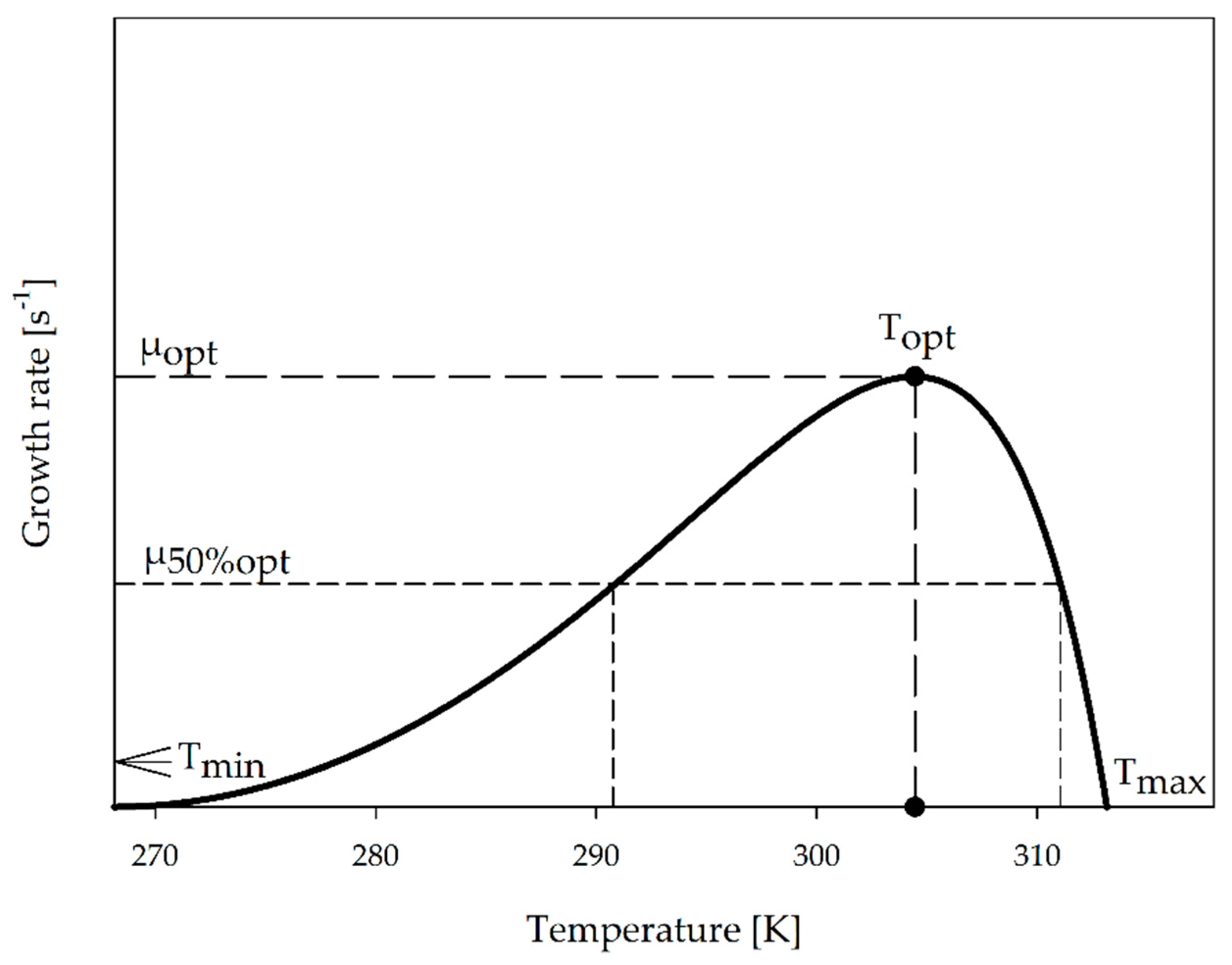
2.3. Characteristic Graph for Growth as a Function of Temperature

Representative curvature of a model depicting the specific growth rate as a function of temperature, called the thermal growth curve, is shown in Figure 2. The simulated optimal specific growth rate (µopt) with the maximum turning point at the temperature optimum (Topt) and growth rate at half of µopt (µ50%opt) are marked in the model of a thermal growth curve. It has been pointed out that the term “optimal temperature” may need further specification to distinguish between the temperature for the optimal growth rate and the optimal temperature of the maximum biomass yield [52]. The minimum and maximum temperatures (Tmin and Tmax, respectively) for growth flank the asymmetric function and mark the thermal tolerance or thermal niche of an organism [53,54]. These three temperatures (Tmin, Topt, and Tmax) are commonly referred to as cardinal temperatures. Bacteria can adapt to changing temperatures in the short run by producing cold- or heat-shock proteins. Furthermore, it was reported that the performance optimum of E. coli can be shifted when exposed to suboptimal temperatures for ~2000 generations. Conversely, the thermal niche breadth remained constant in that case [54]. The result is a reshaped thermal growth curve with the same upper and lower limits. The asymmetry of the thermal growth curve indicates that bacteria, which may be adapted to high temperatures, can survive in lower temperatures quite well. In contrary, fitness decreases sharply when temperatures exceed the optimum, resulting in thermal shock [55,56]. In one of the most recent approaches, the growth of psychrophiles, mesophiles, thermophiles, and hyperthermophiles was modeled, covering a temperature range of 124 °C, from −2 to +122 °C. The model was applied to 230 different strains of uni- and multicellular organisms with growth temperatures below freezing and the highest known temperature for biological growth so far [57,58].

2.4. Mechanistic Versus Empirical Models

An often cited empirical approach for modeling the thermal growth curve of microorganisms is the approach of Ratkowsky et al. [59] (Scopus: cited by 615, 6 November 2019) and the semi-empirical model of Arrhenius. The development of mechanistic approaches for modeling the thermal growth curve of microorganisms started with the master reaction model of Johnson et al. in 1946 [60] (Scopus: cited by 80, 6 November 2019). The mechanistic models consider the description of single essential protein thermal stability (master reaction model) or the thermal stability of the whole proteome (the proteome model) as key for modeling the thermal growth curve. The transition of the native to an active and/or inactive state of the protein is considered. Grimaud et al. have extensively reviewed temperature growth models and concluded that empirical models display a better fit for balanced growth in non-limiting conditions than mechanistic models. Conversely, mechanistic models offer a complementary point of view for modeling thermal growth and can accurately represent temperature responses for growth under non-balanced conditions [61].

3. Temperature Modeling—From the 20th Century until Today

3.1. The Model of Hinshelwood (1946)

Hinshelwood expanded Arrhenius’ model by adding a temperature-dependent term describing a “rate of degeneration” that becomes relevant at temperatures above Topt [62]. Hinshelwood assumes a balanced growth for his model, saying that the total amount of compounds in a cell is constant. The model is based on the assumptions that just one enzymatic reaction is rate-controlling and the product of this reaction is a thermosensitive essential biomolecule which denatures irreversibly when temperatures are raised beyond the optimum. Temperature dependency and denaturation at high temperatures are of zero order and exhibit a temperature dependency similar to the Arrhenius model. The model represents the rate of synthesis in the minuend and degeneration in the subtrahend. At low temperatures, the subtrahend term is insignificantly small; in a small temperature region, both terms are almost equal, canceling each other out; and at high temperatures, the subtrahend term mostly accounts for the rapid decrease of the rate to zero.
µ ( T ) = A 1 · e E 1 R · T A 2 · e E 2 R · T
where A1, and A2 are referred to as pre/non-exponential, collision, or frequency actors, s−1, related to entropy [62]; E1 and E2 are related to enthalpy [22], representing activation energies, J mol−1, of the rate-determining enzyme reaction and high-temperature denaturation, respectively; R is the universal gas constant ~8.314, J mol−1 K−1; and T is the temperature, K.

3.2. The Model of Johnson (1946)

In the same year, Johnson and Lewin [60] proposed another mechanistic model, which also assumes a simple case of a single reaction controlling growth, and called it their “master reaction model”. In contrast to Hinshelwood, they assumed that a reversibly denaturable “master enzyme” E0 controls an essential reaction for growth (assuming no substrate limitation). They reported their observation that E. coli stopped growing at non-viable 45 °C, but started growing exponentially again when transferred back to 37 °C. Increasing the exposition time of E. coli to non-viable temperatures led to lowered growth rates at 37 °C compared to the control. Hence, they assumed and described reversible protein denaturation damage as part of their model by integrating an equilibrium constant (K1). The constant accounts for the equilibrium of reversibly denatured inactive (Ed) to native active enzymes (En).
K 1 =   E d E n
Hence, the amount of native active enzyme is given by Equation (10), with E0 being the total amount of enzyme (native and denatured, mol).
E n =   E 0 1 + K 1 =   E 0 1 + e Δ H R · T · e Δ S R
Johnson and Lewin then referred to Equation (7) proposed by Eyring, adding Equation (10) to account for the amount of active enzyme and substrate concentration and yielding Equation (11) for the temperature-dependent specific reaction rate (k).
k ( T ) =   k B · T h · e Δ S ° / R · e Δ H ° / ( R · T ) · [ S ] · [ E n ]
By assuming that one single enzymatic reaction governs temperature-dependent growth at a constant substrate concentration and by substituting En in Equation (11) with rearranged Equation (10), temperature-dependent growth can be described as Equation (12):
µ ( T )   =   c   · T ·   E 0 · e Δ S ° / R   · e Δ H ° / ( R · T ) · 1 1 + e ( Δ H T · Δ S ) / ( R · T )
where c is a derived Boltzmann/Plancks constant, s K−1, from the Eyring model of Equation (7); Δ H ° and Δ S ° are the standard molar change of enthalpy and entropy of activation, respectively (as described for Equation (7)); Δ H and Δ S are the enthalpy, J, and entropy change, J K−1, respectively, between native and denatured enzymes; R is the universal gas constant ~8.314, J mol−1 K−1; and T is the absolute temperature, K. The equation can then be shortened to the model in Equation (14) using the expression for Gibbs free energy change (between a catalytically active and reversibly denatured inactive state) at a constant temperature (Equation (13)):
Δ G   =   Δ H T · Δ S
µ ( T )   =   C · T   · e Δ H ° / ( R · T ) · 1 1 + e Δ G / ( R · T )
where E0 is assumed to be constant and c · e Δ S ° / R · E 0 is compressed to C. The fraction term containing the Gibbs free energy change can be assumed as the probability that the enzyme is in its native, and not its inactive, state. In the temperature region for a catalytically active enzyme, Δ G , J, has high positive values, yielding almost zero for the exponential term in the denominator of the probability term, and thus one for the probability for a catalytically active enzyme.

3.3. The Model of Sharpe (1977)

In 1977, Sharpe et al. [63,64] merged the models of Johnson and Lewin with the model of Hultin, which were both founded on Eyring’s theory and modeled on the activated complex in chemical reactions [20,60,65,66]. The result was a unified rate model for the description of biological processes at physiological temperatures. Sharpe’s model was originally developed for poikilotherms. Sharpe assumed balanced growth with a constant total amount of compounds per cell and just a single rate-controlling enzyme determining the development rate at all temperatures. Its reaction rate is of a zero order. The total concentration of enzyme (active + inactive) is assumed to be constant at all temperatures. Three enzyme states are considered and described: an inactivation state at low and high temperatures, as well as an active development state. Sharpe described transition between the states by his model, which depicts the thermal growth curve with the following equation:
µ ( T ) = T · e ( Φ   Δ H ° / T ) / R 1 + e ( Δ S L   Δ H L / T ) / R + e ( Δ S H   Δ H H / T ) / R
where T is the temperature, K; is the universal gas constant ~8.314, J mol−1 K−1; and the other parameters describe the rate-controlling enzyme reaction, where Φ is a dimensionless conversion factor; Δ H ° is the enthalpy of activation of the reaction catalyzed by the rate-controlling enzyme, J mol−1; the subscript L accounts for low-temperature inactivation and the subscript H for high-temperature inactivation; and Δ S * , J K−1 mol−1, and Δ H * , J mol−1, mark the entropic and enthalpic change, respectively, upon high- or low-temperature inactivation specified by the subscript. In 1991, Zwietering et al. [8] rewrote the model of Sharpe exhibiting an Arrhenius-type of temperature dependency using activation energies rather than changes in enthalpy to describe growth. As described by the International Union of Pure and Applied Chemistry, IUPAC, the (Arrhenius) activation energy (Ea) and enthalpy of activation are not the same, but approximately equal, as they are convertible, depending on the molecularity [22].
µ ( T ) = k a · e E a R · T 1 + k l · e E l R · T + k h · e E h R · T
where ka (s−1), kl (-), and kh (-) are collision factors that are dimensionless in the denominator, as described by Zwietering et al. [8]; E, J mol−1, represents the activation energy; subscript a accounts for the rate-determining enzyme reaction; subscripts h and l describe high- and low-temperature inactivation, respectively; R is the gas constant ~8.314, J mol−1 K−1; and T is the temperature, K.

3.4. The Model of Mohr (1980)

Mohr and Krawiec [24] analyzed the thermal growth curves for 12 bacterial species. Among them were thermophiles, mesophiles, and psychrophiles. They used the Arrhenius plot for their data, where ln(µ) is plotted against the reciprocal temperature in Kelvin. They reported two different slopes for the Arrhenius profiles for some mesophiles and thermophiles at suboptimal temperatures. The temperature at the interception point were both slopes meet is referred to as the “critical temperature” (Tcrit) [24,67]. This point marks the turning point where the organization of an organism, and hence it growth behavior, changes. In order to describe the two different slopes, they proposed two equations, which they reduced to one with the assumption that “[…] a balance of organizations exists at any temperature”:
µ ( T ) = A 1 · e E 1 / R · T A 2 · e E 2 / R · T T crit   < T   <   T max
µ ( T ) = A 1 · e E 1 / R · T T min   < T   <   T crit
µ ( T ) =   1 A 1 * · e E 1 / R · T + A 1 * * · e E 1 / R · T A 2 · e E 2 / R · T
where A 1 , A 1 , and A 2 are referred to as pre/non-exponential, collision, or frequency actors, s−1; E 1 , E 1 , and E 2 are referred to as temperature characteristics, J mol−1; R is the gas constant ~8.314, J mol−1 K−1; and T is the temperature, K. The parameters marked with a “ ’ ” are used to describe temperature-dependent growth for T min   <   T   <   T crit , whereas parameters without “ ’ ” are used to describe temperature-dependent growth for T crit   <   T   <   T max , A 1 * = 1/ A 1 , and A 1 * * = 1/ A 1 .

3.5. The Model of Schoolfield (1981)

Schoolfield developed a non-linear regression model [68] based on the model proposed by Sharpe. His group reformulated the model of Sharpe and eliminated the high correlations of Sharpe’s parameters (e.g., 0.9996). Furthermore, Schoolfield et al. argued that there is no “readily apparent” initial guess for beginning iterations for parameter estimation. Hence, they also aimed to facilitate the regression process and parameter estimation.
µ ( T ) = µ 25 · T 298 · e [ Δ H ° R · ( 1 298 1 T ) ] 1 + e [ Δ H L R · ( 1 T 1 / 2 L 1 T ) ] + e [ Δ H H R · ( 1 T 1 / 2 H 1 T ) ]
Schoolfield et al. chose 25 °C (298 K) and the respective specific growth rate µ 25 , s−1, as a reference because enzyme inactivation would be low or not present at that temperature in most biological systems. Δ H ° is the enthalpy of activation of the reaction catalyzed by the rate-controlling enzyme, J mol−1; the subscript L accounts for low-temperature inactivation and the subscript H for high-temperature inactivation of the enzyme; and Δ H * marks the enthalpic change upon high- or low-temperature inactivation specified by the subscript, J mol−1. With an increasing or decreasing temperature, 50% of the rate-controlling enzyme is inactivated by either a high T 1 / 2 H , K or low temperature T 1 / 2 L , K, as previously described by Hultin [66] and adopted by Schoolfield et al. [68].

3.6. The Models of Ratkowsky and Zwietering (1982–1991)

As extensively reviewed by Grimaud et al. [61], several models for temperature-dependent growth in biological systems have been developed. Most of these models were developed to describe food spoilage and medical applications. One often cited (802, Scopus, 8 August 2019) empirical model is the square root model proposed by Ratkowsky et al., as an alternative to the widely used Arrhenius model, to describe growth as a function of temperature [26]:
µ ( T ) = [ b 1 · ( T T min ) ] 2
where b1 is a Ratkowsky parameter, K−1 s−0.5, and Tmin is the minimum temperature of growth, K. This model was extended to the complete bio-kinetic range in 1983 by the same author [59]:
µ ( T ) = ( b 2 · ( T T min ) · { 1 e [ c 2 · ( T T max ) ] } ) 2
where c is a Ratkowsky parameter, K−1, and Tmax is the maximum temperature, K, at which growth is observed. Zwietering et al. [8] argued that Ratkowsky’s model could not be used for temperatures above Tmax because the model predicted positive values for growth rates beyond the high-temperature end of the thermal niche. They therefore adapted the model accordingly and the result is shown in Equation (23).
µ ( T ) = [ b 3 · ( T T min ) ] 2 · { 1 e [ c 3 · ( T T max ) ] }

3.7. The Model of Roels (1983)

In 1983, Roels et al. [69] developed a model to describe the growth rate as a function of temperature. The numerator has an Arrhenius-type appearance and the energy for activation was replaced by the Gibbs free energy change upon denaturation of a rate-controlling enzyme in the denumerator.
µ ( T ) = A · e ( E G R T ) 1 + B · e ( Δ G d R T )
where A and B are pre-exponential factors, s−1; R is the gas constant ~8.314, J mol−1 K−1; and T is the temperature, K.

3.8. The Model of Davey (1989)

Davey proposed an empirical generalized predictive model based on a modified linear-Arrhenius equation, which combined the influence of temperature and water activity to describe microbial growth [70]. The activation energy parameter from the original Arrhenius model was replaced in Davey’s model by two coefficients of inverse temperature. In his work, Davey provided and evaluated models for the influence of environmental factors like the aw value or pH in combination with temperature, as well as temperature as the sole influencing factor, on growth [70,71,72]. The model describing temperature as the sole environmental factor is shown in Equation (25):
µ ( T ) = e C 0 + C 1 / T + C 2 / T 2
where C0C2 are dimensionless Davey coefficients, - and the energy of activation given in the Arrhenius equation is replaced by two parameters of reciprocal temperature, K. Two years later, in 1991, Davey used the model for predicting the temperature-dependent lag time [72].

3.9. The Models of Lobry and Rosso (1991–1993)

In 1991, Lobry [73] developed an empirical model that includes the three cardinal temperatures (Tmin, Topt, and Tmax) as parameters. The cardinal temperature model (CTM) estimates positive values for growth rates at temperatures between the low temperature and high temperature end (Tmin and Tmax), with the highest growth rate ( µ opt (s−1)) at Topt. Outside the thermal niche (T < Tmin; T > Tmax), negative values are predicted. Each microbial species exhibits these three characteristic cardinal temperatures, which permits direct biological interpretation of the model parameters and facilitates parameter estimation using experimental data for Lobry’s CTM-model Equation (26). The authors emphasize the “absence of high structural correlations” between parameters of their model. In 1991, Rosso et al. [74] further elaborated Lobry’s empirical model by including the point of inflection in the suboptimal range of temperatures, which was experimentally determined. Following this, the so-called cardinal temperature model with inflection (CTMI; Equation (27)) could be used to accurately predict growth in the suboptimal range of temperature. Rosso’s group noted an “unexpected” high linear correlation between cardinal temperatures, especially between Tmax and Topt, with r = 0.991. They then argued that due to the correlations found, one instead of three cardinal temperatures could sufficiently describe the permissive temperature range for growth. They also mentioned an exception for the stated relationships between the cardinal temperatures for the growth behavior of Vibrio sp. In total, they analyzed 47 different data sets describing the growth of psychrophilic, mesophilic, and thermophilic strains.
µ ( T ) = µ opt · [ 1 ( T T opt ) 2 ( T T opt ) 2 + T · ( T max + T min T ) T max · T min ]
µ ( T ) = µ opt · ( T T max ) · ( T T min ) 2 ( T opt T min ) · [ ( T opt T min ) · ( T T opt ) ( T opt T max ) · ( T opt + T min 2 · T ) ]  

3.10. The Model of Blanchard (1996)

Blanchard et al. [75] originally developed their model to quantify the short-term temperature effect on natural assemblages of microphytobenthos’ photosynthetic capacity. Blanchard described a progressive increase in photosynthetic capacity during a temperature increase up to an optimum temperature, with a rapid decrease when the temperature was raised beyond the optimum. For the model, cardinal temperatures (Tmin, Topt, and Tmax) with a biological meaning are used to facilitate a reasonable initial guess for parameter estimation. Grimaud et al. [61] rewrote the Blanchard model to represent growth as a function of temperature instead of photosynthetic capacity, as shown in Equation (28):
µ ( T ) = µ opt ( T max T T max T opt ) β · e β · ( T opt T ) / ( T max T opt )
where µopt, s−1, is the maximal specific growth rate at optimal temperature Topt, K; Tmax, K, is the maximum temperature where growth is observed; and β is a dimensionless Blanchard parameter.

3.11. The Models of Eppley and Norberg (2004)

Eppley [76] proposed a simple function with a positive exponential correlation between temperature and maximum expected growth, as shown in Equation (29). He stated that this model may be used for a generalized estimate for µmax in unicellular algae for temperatures <40 °C.
µ ( T )   =   0.851 · 1.066 T
The proposed Eppley curve or envelope function of Equation (29) shows the evolutionary interspecific upper limit for the maximum specific growth rate at any temperature up to 40 °C. The limit for the maximum growth rate increases exponentially until 40 °C in Eppley’s function. For model assembly, Eppley used almost 200 data points of different species of unicellular algae [76]. Based on Eppley’s findings, Jon Norberg developed a model for temperature-dependent growth in 2004 [77], shown in Equation (30).
µ ( T ) = [ 1 ( T Z w ) 2 ] · 0.59 · e 0.0633 · T
An envelope function 0.59 × e0.0633T according to Eppley is contained in Norberg’s model for temperature-dependent growth, where T, K, is the ambient temperature and Z, K, is the temperature with the maximum specific growth rate derived from the envelope function representing Topt respectively. The width of the temperature response function is determined by the parameter w, K, meaning the width of the thermal niche. A generalized form of the Eppley–Norberg model Equation (31) would add a and b as dimensionless parameters, -, generalizing the Eppley envelope function.
µ ( T ) = [ 1 ( T Z w ) 2 ] · a · e b · T

3.12. The Modified Master Reaction Model (2005)

In 1967, Brandts recognized that the master reaction model proposed by Johnson and Lewin (see Equation (12)) failed to describe enzymatic reactions adequately when applied to the full bio kinetic temperature range [78,79]. Arguably, the limitations of the model arise from the assumed temperature independence of Δ G in the master reaction model upon protein denaturation. Therefore, Brandts et al. attributed the temperature dependency to Δ G by simply using an empirical polynomial expression relating Δ G to T. In 1974, Privalov et al. [80] reported a linear relation between enthalpy and entropy and temperature upon protein unfolding when assuming a specific constant heat capacity change for a specific protein. Almost 20 years later, it was reported that the change in enthalpy upon denaturation ( Δ H d ) normalized to the number of amino acid residues (or molecular weight, respectively) at a specific temperature ( T H * ~373 K) converged to a common value ( Δ H * ). Likewise, the same convergence behavior to one common value ( Δ S * ) at a specific temperature ( T S * ~385 K) for entropy upon denaturation ( Δ S d ) normalized to the number of amino acid residues was described for a number of homologous compounds [80,81,82,83]. The so-called convergence temperatures ( T H * and T S * ) were obtained as the temperatures where the apolar contributions (apolar hydrogen atoms CH) to the corresponding changes in entropy or enthalpy, respectively, upon denaturation approach zero [81,82,84]. Therefore, Δ H * describes only polar and van der Waals interactions and Δ S * primarily accounts for configurational entropy [83]. In 1990, Murphy et al. [81] analyzed the convergence behavior by plotting Δ H d or Δ S d normalized to mol amino acid residue against the normalized heat capacity change ( Δ C p ) upon denaturation and obtained the following correlations:
Δ S d = Δ S * + Δ C p · l n ( T T S * )
Δ H d = Δ H * + Δ C p · ( T T H * )
The above-mentioned equations describe a temperature-dependent enthalpic and entropic change upon denaturation normalized to the number of amino acid residues in a protein (n). From Murphy’s findings [81], the change in Gibbs free energy upon protein denaturation (~protein thermal stability) is given by
Δ G d ( T ) = n · [ Δ H * T · Δ S * + Δ C p · [ ( T T H * ) T · l n ( T T S * ) ] ]
where Δ C p · [ ( T T H * ) T · l n ( T T S * ) ] accounts for the hydrophobic contribution of the Gibbs free energy change upon denaturation of the rate-determining “master enzyme”. Ross connected Murphy’s findings with the rewritten master reaction model of Johnson and Lewis, where the change in enthalpy between the catalytically active and inactive state of the rate-limiting enzyme was replaced by the temperature-dependent Gibbs free energy change [79,85].
µ ( T ) = c · T · e ( Δ H ° / R · T ) 1 + e ( Δ G d / R · T )
Replacing the description of the Gibbs free energy in the denominator of Equation (35) with the term in Equation (34) resulted in a modified master reaction model:
µ ( T ) = c · T · e ( Δ H ° / R · T ) 1 + e ( n · { Δ H * T · Δ S * + Δ C p · [ ( T T H * ) T · l n ( T / T S * ) ] } / R · T ) .
In the denominator of Equation (36), the thermodynamic parameters Δ H * , Δ S * , and Δ C p are normalized to mol amino acid residue. In 2005, Ratkowsky et al. [79] reduced the eight-parameter model given in Equation (36) to a five-parameter model by simply applying the universal constants for globular proteins T H * = 373.6 K, T S * = 385.2 K, and Δ S * = 18.1 J K−1 found by Murphy et al. [81,82] to the model. Ratkowsky’s group fitted the reduced five-parameter modified master reaction model to data from 35 bacterial strains. The universal constant Δ H * suggested by Murphy’s group with 5640 J mol−1 amino acid residue was found to be unsuitable for representing bacterial growth when applied to five data sets of Ross [86]. The reduced modified master reaction model with applied universal constants evaluated in the work of Ratkowsky et al. [79] is given in Equation (37).
µ ( T ) = c · T · e ( Δ H ° / 8.314 · T ) 1 + e ( n · { Δ H * T · 18.1 + Δ C p · [ ( T 373.6 ) T · l n ( T / 385.2 ) ] } / 8.314 · T )

3.13. The Model of Zeldovich (2007–2016)

The group of Zeldovich [87] argued that the whole proteome has to be considered when describing the temperature response and sensitivity of an organism. Ghosh and Dill [88] continued the work of Zeldovich et al. and proposed a model that considers the folding stabilities across an organisms’ proteome to describe temperature-dependent growth rates of bacteria. They assumed that the growth rate was a function of temperature composed of a product of two factors: First, Arrhenius-type low-temperature activation for one or more activated metabolic processes controlling the increase of growth rate at low temperatures, and second, a term accounting for the folded part of the proteome at any temperature, which also depicts the “denaturation catastrophe” when reaching high temperatures.
µ ( T ) = µ 0 · e ( Δ H ° k · T ) i = 1 Γ 1 1 + e ( Δ G un ( N i , T ) / R · T ) ,
where µ0 is a growth rate reference, s−1. The parameter Δ H ° , J mol−1, describes the activation barrier for growth (e.g., an essential growth-limiting metabolic rate). The authors found that the activation barrier for growth (~68.2 kJ mol−1) in E. coli approximately corresponds to the energy needed by ribosomes to form a peptide bond. Hence, the authors identified ribosomal action to grow protein chains as one of the key growth rate-limiting factors, along with protein motions necessary for enzymatic reactions. Γ describes the amount of essential proteins required for growth. The product term accounts for the probability that the ith essential protein composed of Ni amino acids is in its native state, which is expressed by Δ G u n in Equation (39):
Δ G u n = k B · T 0 · n · [ g 0 + m 1 · c k B · T 0 + Δ C p k B · T 0 · ( T T H * ) + T T 0 · l n ( z ) T T 0 · Δ C p · l n ( T T S * ) + l b 2 · n · ( Q n 2 R n · ( 1 + κ · R n ) Q d 2 R d · ( 1 + κ · R d ) ) ]
where kB is the Boltzmann constant ~1.381 ⋅ 10−23, J K−1; T0 = 300 K; n is the number of amino acids with respective to the chain length of a protein; g0 is the free energy upon amino acid desolvation and upon contact; c is the concentration of denaturant; Δ C p is the heat capacity change upon denaturation, J K−1 mol-residue−1; T is the absolute temperature, K; T H * = 373 K and T S * = 385 K are the enthalpic and entropic convergence temperatures, respectively; z is defined as the loss of average conformational freedom per backbone bond; lb is the average Bjerrum length; Qn and Qd are the total net charge of native and denatured protein, respectively; Rn and Rd account for the radii of native and denatured protein, respectively; κ is the reciprocal of the Debye length (for further details, see [89,90]). To obtain the probability distribution for protein stabilities of a proteome p( Δ G ), Equation (39) can be used. The equation accounts for the stability of an average single protein of length n and may be used in combination with the distribution of protein chain lengths (P(n)) of a cell available for various cell types from genomic/proteomic data in order to calculate temperature-dependent proteome stability.

3.14. The Model of Daniel (2010)

In 2010, Daniel et al. [91] proposed the equilibrium model to describe temperature-dependent catalytic activity of enzymes in non-limiting conditions. The group reported that the decrease of the catalytic rate constant (kcat) of tested enzymatic reactions above the optimal temperature (Topt) does not entirely correspond to thermal stability data and irreversible denaturation. Furthermore, they found that part of the activity loss above Topt was reversible and probably associated with a “conformational, dynamic and solvent-based effect” altering the active site of the enzyme. To explain the higher than expected decrease of kcat at a certain temperature, they suggested that an enzyme may be present in three states: (i) catalytically active (Eact); (ii) catalytically inactive, but not (significantly) unfolded (Einact); and (iii) irreversibly denatured (X). They rapid changes of the Michaelis constant (Km), describing an enzyme’s affinity towards a substrate, that occur with temperature support their hypothesis of an “Einact state”, where the active site is altered. They argue that the active site may need a certain degree of flexibility to function properly and is therefore more prone to changes in temperature affecting conformation and dynamics.
E act   K e q E inact k inact X
Daniel’s group assumed a rapid equilibrium between Eact and Einact and time-dependent denaturation at a certain temperature. The conversion rate of Eact to Einact is thereby assumed to be faster than the rate of denaturation and catalytic reaction rate, respectively. The authors investigated the applicability of the model for >50 datasets of >30 enzymes of different reaction classes and structures (monomeric to hexameric) and concluded that their model is universally applicable and independent of the reaction type and enzymatic structure [91]. The model may therefore be suitable for describing a thermal growth curve, where a rate-controlling enzymatic reaction is often assumed to describe temperature-dependent growth (e.g., master reaction model, [60]).
µ ( T ) = k B h · T · E 0 · e ( Δ G cat * R · T ) · e [ k B h · T · e ( Δ G inact * R · T ) · e ( Δ H eq · ( 1 T eq   1 T ) / R ) · t 1 + e ( Δ H eq · ( 1 T eq   1 T ) / R ) ]   ·   [ 1 + e ( Δ H eq · ( 1 T eq     1 T ) / R ) ] 1
where kB is the Boltzmann constant ~1.381 ⋅ 10−23, J K−1; h is the Planck’s constant ~6.626⋅10−34, J s−1; T is the absolute temperature, K; E0 is the total enzyme concentration composed of the sum of Eact, Einact, and X, mol m−3; Δ G cat * is the Gibbs free energy of activation of the enzymatic reaction; R is the universal gas constant ~8.314, J mol−1 K−1; Δ G inact * is the Gibbs free energy of activation for the irreversible denaturation of the rate-controlling enzyme; Δ H e q is the enthalpic change between Eact and Einact; T e q is the equilibrium temperature where the rate-controlling enzyme is present as 50:50 Eact and Einact, K; and t is the time, s.

3.15. The Model of Kooijman (2010)

The DEB or Dynamic Energy Budget theory deals with the description of rates for physiological processes. Assimilation, growth, respiration, maintenance, or reproduction in individual, not further specified, “organisms” are analyzed and described by the generalized theory. The rates are described as a function of the environment, like the temperature or nutrient availability, and the state of the organism like size or age, for example. S.A.L.M. Kooijman, whose early concepts on energy budgets were published in 1986 [92], summarized his work in “DEB theory for Metabolic Organization” in 2010 [93]. In DEB theory, temperature-dependent growth is described by a reformulated Arrhenius equation in the numerator and complemented by a term inspired by Sharpe’s model [63] for reduced rates at the high- and low-temperature end in the denominator. The equation therefore accounts for the amount of enzyme in its native state and considers a possible transition to an inactive state via hot and cold denaturation. Kooijman argues that Eyring’s thermodynamic interpretation of the Arrhenius type of temperature dependence might only be understood as an approximation. It is an enormous step from Eyring’s model, considering bimolecular reactions in the gas phase, to physiological rates with many compounds [94].
µ ( T ) = k 1 · e T A / T 1 T A / T 1 + e T A l / T T A l / T l + e T A h / T h T A h / T
where T1 is a reference temperature, K, with the corresponding rate k1, s−1; TA is the Arrhenius temperature (i.e., linear slope of the Arrhenius plot), K; Tl and Th mark the cardinal temperatures flanking the thermal niche (low- and high-temperature denaturation, respectively), K; and TAl and TAh account for Arrhenius temperatures at temperature boundaries of the thermal niche, K.

3.16. The Model of Huang (2011)

The group of Huang [95] developed a model by modifying and combining the Arrhenius equation with the theory and model of Eyring et al. [4,20,65].
  µ ( T ) = A · T · e ( Δ G R · T ) α
where Δ G , J mol−1, accounts for an energy term; R is the universal gas constant ~8.314, J mol−1 K−1; T is the absolute temperature, K; α is a Huang parameter, K−1; and A describes the collision or frequency factor, s−1. Huang reports that their model can only sufficiently describe growth behavior at a suboptimal temperature. To extend their model to the entire physiological temperature range, they used an expression known from Ratkowsky et al. [59]:
  µ ( T ) = A · T · e ( Δ G R · T ) α · [ 1 e c 2 · ( T T m a x ) ]
where c2 is a Ratkowsky parameter, K−1, and Tmax is the maximum growth temperature, K. Huang’s group reported good fits (R2 = 0.985) for their model using data for thermal growth rates from five different bacteria.

3.17. The Model of Corkrey (2014)

In 2014, Corkrey et al. attempted to build a universal mechanistic model [58]. It was used to model the growth of 230 different strains of unicellular and multicellular organisms ranging from psychrophilic to hyperthermophilic, covering a temperature range of 124 °C, from −2 °C to +122 °C. They therefore argued that their findings might be used to model the dependence of the growth rate on temperature for all unicellular and multicellular life forms. Being able to find a good fit for their universal model to the thermal growth curves of various life forms, they concluded that there might be evidence for the presence of a single highly conserved reaction in the last universal common ancestor. Under all limiting conditions, a single-enzyme-catalyzed reaction rate, which controls the growth rate, is described in the numerator of the Corkrey model by an Arrhenius type of temperature dependency. The denominator accounts for the effects of temperature on protein conformation, which causes alterations in catalytic activity of the putative enzyme and therefore a change in the expected rate.
µ ( T ) = T · e ( c Δ H ° R · T ) 1 + e ( n · Δ H * T · Δ S * + Δ C p · ( T T H * T · l n ( T / T S * ) ) R · T )
where Δ H ° is the enthalpy of activation, J/mol; R is the universal gas constant ~8.314, J mol−1 K−1; c is a dimensionless scaling factor; T is the temperature, K; Δ C p is the heat capacity change, J K−1 mol−1 -amino acid residue, upon denaturation of the putative enzyme; Δ H * is the change of enthalpy, J mol−1 amino acid residue, at the convergence temperature T H * , K, for enthalpy of protein unfolding; and Δ S * is the change of entropy, J K−1, at the convergence temperature T S * , K, for the entropy of protein unfolding.

3.18. The Model of Hobbs (2014)

The heat capacity model or macromolecular rate theory was proposed by Hobbs et al. [96] and applied by Schipper et al. [97]. They state that enzymatic rates show Arrhenius behavior when increasing with temperature, until an optimum (Topt), but argue that decreasing rates above Topt cannot sufficiently be explained only by denaturation of the enzymes. They have reported the effect of a heat capacity change upon activation (between the ground state and transition state of a rate-limiting enzyme) that shapes the thermal growth curve. The change in heat capacity affects the temperature dependency of Δ G °   (Gibbs free energy difference, between a ground state and transition state) that is in turn responsible for determining the temperature dependency of enzymatic activity. They state that the change in heat capacity influencing enzymatic rates implicates temperature dependence for various biological rates, ranging from “enzymes to ecosystems”. Hobbs et al. formulated their findings using Eying’s Equation (46) as a scaffold and a term to describe the degree of temperature dependence of Δ G ° with Δ C p ° Equation (47). Assuming Δ C p ° to be zero, Δ G ° would be independent from temperature and the reaction behavior of the growth rate-limiting enzyme would follow an Arrhenius type of temperature dependence. Large negative values for Δ C p ° would lead to a significant temperature dependence of Δ G ° , leading to a non-Arrhenius behavior and explaining a decrease in reaction rate above Topt, independent of denaturation. Compared to the master reaction model, heat capacity theory takes into account that enzymes are in fast equilibrium with the transition state and denaturation does not easily occur [61,96,97].
µ ( T ) =   k B h · T · e ( Δ G ° ( T ) / R · T )
Δ G ° ( T ) =   Δ H T 0 ° + Δ C p °   · ( T T 0 ) + T · ( Δ S T 0 ° + Δ C p ° · l n ( T T 0 ) )
where kB is the Boltzmann constant ~1.381 ⋅ 10−23, J K−1; h is the Planck’s constant ~6.626⋅10−34, J s−1; Δ G ° is the Gibbs free energy difference, between a ground state and transition state, J mol−1; R is the universal gas constant ~8.314, J mol−1 K−1; T is the absolute temperature, K; T0 is a reference temperature, K; Δ H T 0 ° and Δ S T 0 ° are enthalpic and entropic change between reactants and the transition state at the reference temperature T0; Δ C p ° is the heat capacity change between reactants and the transition state, J mol−1 K−1.

3.19. The Model of DeLong (2017)

In 2017, DeLong et al. [98] argued that models describing the thermal growth curve lack the assumption that the catalyzing enzyme lowers the activation energy of the rate-determining reaction. They therefore introduced a model that describes the reduction of required activation energy for the rate-determining reaction as a function of free energy (enzyme stability) of the catalyzing enzyme. This term was incorporated into the dividend of the exponential term of the Arrhenius function. The Arrhenius activation energy (Ea; see Equation (4)) was replaced with the difference of a baseline energy (Eb, J), describing kinetic requirements as if the reaction would take place outside an organism, lowered by the enzymatic contribution (Ec, J) inside an organism, yielding Equation (48):
µ ( T ) = A · e ( E b E c ) k B · T
where the authors used the Boltzmann constant kB ~1.381 ⋅ 10−23, J K−1, instead of the universal gas constant in the divisor of the exponential term and T is the absolute temperature, K. The dividend of the exponential term then accounts for the activation energy lowered by the enzymatic action. The extent of enzymatic contribution (Ec) depends on the activity status of the enzyme, which is given by probability terms of protein stability. The temperature-dependent protein stability is given by Δ G (Equation (49)), where Δ H , J, is the change of enthalpy and Δ C p , J mol−1 K−1, the change in heat capacity, both relative to the melting temperature Tm, K, between the folded and unfolded state. At Tm, Δ H is by definition zero and increases for temperatures below Tm. Δ C p reflects the extent of free energy that can be kept by the enzyme without changing the temperature, which increases below Tm with a decreasing temperature. The authors assumed that the probability of the maximum contribution of the enzyme to reduce the activation energy by the amount EL approaches 1 at Δ G max . Hence, the probability function Equation (50) is composed of the maximum amount (EL) by which an active enzyme can lower the activation energy and the probability of the enzyme being correctly folded and active, given by the ratio of Δ G to Δ G max . This transformation yields probability terms for each parameter in Equation (49), as presented in Equations (51) and (52). Therefore, Equation (49) can be rewritten as Equation (53).
Δ G =   Δ H · ( 1 T T m ) + Δ C p · ( T T m T · l n ( T T m ) )
E c =   E L · Δ G Δ G max
E Δ H = E L · Δ H Δ G max
E Δ C p = E L · Δ C p Δ G max
E c =   E Δ H · ( 1 T T m ) + E Δ C p · ( T T m T · l n ( T T m ) )
Combining the probability function Equation (53) for the degree of enzymatic contribution to lowering the baseline energy Eb of the rate-determining reaction with the Arrhenius-type Equation (48) yields the enzyme-assisted Arrhenius model in Equation (54).
µ ( T ) = A · e ( E b ( E Δ H · ( 1 T T m ) + E Δ C p · ( T T m T · l n ( T T m ) ) ) ) k B · T

3.20. Additional Temperature Models

In Table 1 further models describing a hunchback-shaped curve for temperature-dependent rates are summarized.

4. Biotechnological Applications for Targeted Temperature Variation Assisted by Temperature Models

4.1. Temperature with Potential for Bioprocess Design

Temperature is an easily measurable (continuously, in situ, and in real-time) and controllable process variable. In most cases, temperature is controlled at constant values to maintain suitable physiological conditions at a given optimum value. Besides temperature, these requirements are also common for other basic physico-chemical characteristics, including dissolved oxygen and the pH value, which are routinely controlled in most bioreactor cultivations. For bioprocess design and optimization, very few correcting variables (e.g., the addition of fresh feed media) are available to direct a bioprocess towards a desired outcome. There are two strategies for efficiently using the temperature to influence the process outcome. First, alterations in the process temperature may be used to target metabolism, deliberately trigger stress responses, modify enzymatic turnover, or activate existing regulatory mechanisms. Secondly, natural or synthetic regulation mechanisms may be introduced to engineer host microorganisms (see Section 2.2). As such, processes can be designed to include these regulatory mechanisms as an effective tool to influence the process. Even though several systems inducible by temperature have been discovered and made available to biotechnologists in the last decades, only very few have been applied for process design or optimization [12].

4.2. Application of Temperature Models and Temperature for Bioprocesses Design

Mukhtar et al. modeled the temperature-dependent soil nitrification potential rate with the square root model of Ratkowsky et al. and estimated the optimum temperature for the nitrification potential rate with the heat capacity model. The authors suggest that the knowledge of thermodynamic properties of the soil nitrification response may be used to improve the application of large-scale fertilization, while reducing eutrophication and connected negative environmental impacts [105]. For cleaning purposes of contaminated water with excess nitrogen, denitrifying fixed-bed bioreactors can be used for NO3 removal [106]. The group of Nordström et al. used the Eyring equation to simulate the temperature dependency of NO3 removal rates in a denitrifying fixed-bad wood chip bioreactor [107]. They used the heat capacity model of Hobbs et al. [96] to derive the optimum temperature for NO3 removal by their bioreactor. Nordström et al. reported that NO3 removal rates of reducing microbial consortium change over time, while the temperature optimum is shifted towards lower temperatures (from 24.2 to 16.0 °C) [107]. Downshifts in temperature may somewhat be beneficial for a bioprocess, depending on the intended outcome. Seel et al. were able to increase biomass yields to optimize nutrient assimilation at suboptimal temperatures (10 °C) for mesophilic isolates from chilled foods and refrigerators in defined medium compared to their reference strains [52]. They emphasized the importance of defining the “optimum temperature”. Seel et al. distinguish between the optimum temperature for the maximum growth rate and the optimum for the maximum biomass yield. At 10 °C, which was around 15–25 °C below the optimum for the maximum growth rate of isolates, they reported an increase of 20%–110% of biomass formation. They argue that the generally assumed optimum growth temperature at µmax may not be the optimum for all biological processes in the host. This has been described for protein production, membrane permeability, and cellular stress [108,109,110,111,112]. The works of Corkrey et al. [58,113] thermodynamically justified the applied findings of Seel et al. Corkrey’s model described the connection between the temperature stability of proteins and the growth rate governed by an assumed essential enzymatic reaction, with the temperature for optimal enzyme stability being 10–15 °C below the temperature of µmax. Seel et al. state that due to correct protein folding and protein turnover, energy can be conserved and the biomass yield improved. Perhaps the most popular example for altering temperature as a means of an optimized process outcome can be found during the production of recombinant protein, such as by using E. coli as a heterologous expression system [12]. During the process, typically at the stage of the induction of protein expression, a temperature shift is performed, lowering the process temperature by several °C. This temperature shift does not benefit overall transcription or translation activity, but instead, results in an increased amount of correctly folded protein. This is due to lower amounts of recombinant protein being less likely to form inactive, insoluble aggregates (inclusion bodies), and allowing more time for correct folding after translation due to lower protein production rates. In the case of enzyme production, correctly folded protein is a prerequisite of enzymatic activity, and therefore, in most cases, temperature shifts are applied [114]. Another possibility for using temperature as a method for optimizing protein production is the application of thermo-inducible promoter systems. Considering the perspective of bioprocess engineering, it is of high interest to combine strain engineering and process development approaches to maximize overall productivity and yields. Strong chemically inducible promoters and expression systems that are commonly used in laboratory-scale protein expression [115] cause a high degree of metabolic burden to the microorganisms, and as such, protein production results in a simultaneous reduction of growth. It is therefore beneficial for optimized process design to be able to uncouple biomass growth from protein biosynthesis. Furthermore, production of recombinant proteins at early stages of cultivation often results in reduced overall yields, as many proteins are sensitive to degradation by proteases [114,116]. To counteract this instability of recombinant proteins, inducible promoter systems are a possible tool. Thermo-inducible promoter systems have the advantage of not requiring intrusion into the process, as chemical inductors are not required. As such, the risk of contamination, as well as the costs of the process, may be reduced. Nalley et al. evaluated the effect of temperature on growth, fatty acid production, and the fatty acid profile for algae suitable for mass cultivation and biofuel production [117]. They assessed the effect of temperature on microalgae with the model of Norberg [77]. Nalley et al. report temperature-specific fatty acid production, which is mostly controlled by the temperature-dependent growth rate. Furthermore, they found that temperature dramatically influences the fatty acid profile, with an increase in polyunsaturated fatty acids and decrease in monounsaturated and short fatty acids when increasing the temperature. The thermostable phosphotriesterase-like lactonases (PLLs) from hyperthermophilic Sulfolobus genera present an industrially relevant molecule for bioremediation processes, such as in the degradation of highly toxic pesticides like organophosphates [118]. Thermostable PLLs are of particular interest due to their wide temperature and pH working range, as well as resistance to organic solvents. In contrast to mesophilic enzyme isolates, the application of extremozymes is not prone to low stability in solution or an elevated temperature (>30 °C) [119,120]. In the work of Restaino et al., a high-yield pre-industrial-scale process with an optimized purification method for PLLs was developed [11]. The authors exploited the thermostability of PLLs in their downstream and recombinant PLL production in fast-growing mesophilic E. coli for their upstream and bioproduction strategy. Impurities were removed by a thermo-precipitation step (65–75 °C), which was optimized using a statistical response surface method to compute optimal precipitation temperatures. The solubility of proteins can be altered by different variables, like the pH, protein concentration, ionic strength, or temperature. Ethanol may be used as a solvent for precipitation, but exhibits the tendency to denature proteins at temperatures above 0 °C. Therefore, cold EtOH is often used for protein fractionation [121]. The authors Cimini et al. investigated the influence of temperature on the industrially relevant capsular polysaccharide (CPS) of E. coli, K4 [122]. It exhibits a high similarity to the economically valuable but only expensively extractable chondroitin from animal tissue. Chondroitin is, for example, used in the pharmaceutical sector to prevent osteoarthritis [123]. Cimini et al. found a positive correlation between CPS production and temperature. As stated before, CPS production is thermoregulated and E. coli CPS are not expressed at temperatures <20 °C [124]. Another pharmaceutically relevant product and precursor for the commonly used anti-inflammatory drug desfluorotriamcinolone, is 16 α -hydroxy hydrocortisone. Hydrocortisone is converted in a temperature-dependent manor by Streptomyces roseochromogenes to 16 α -hydroxy hydrocortisone. The group of Restaino et al. was able to maximize the bioconversion of hydrocortisone to 16 α -hydroxy hydrocortisone, while lowering side-product formation. By adjusting the process temperature to 26 °C and pH to 6, they were able to almost entirely (95%) convert hydrocortisone into the desired product 16 α -hydroxy hydrocortisone [125]. Another example for lowering the temperature to obtain optimal expression, correctly folded, and working recombinant enzymes is the mammalian enzyme 6-O-sulfotransferase (6-OST). It can be recombinantly produced in E. coli. 6-OST is of particular interest as it is required for the industrial and biotechnological production of heparin. So far, the blood anticoagulant heparin has only been derived from animals. 6-OST side-specifically sulfonates a heparin precursor and marks a key step in heparin bioproduction. The group of Restaino et al. reported high cell density cultivation of E. coli in which recombinant mammalian 6-OST was produced using an induction strategy optimized for yield and productivity. The strategy involved lowering the temperature (37 to 25 °C) upon induction and using a combination of two inducer molecules to balance the metabolic burden. The combination of balanced biomass growth and the induction strategy resulted in an optimal recombinant enzyme expression and enhanced biomass productivity [126].
An interesting application involving measuring and controlling the temperature during bioprocesses is the estimation of metabolic activity by heat balancing. In a partially isolated bioreactor system, heat generation by metabolic processes can be calculated by measuring heat transfer from or to the bioreactor [5]. This calorimetric technique typically involves the calculation of a heat balance by calculating transfer from or to the heat exchanger, enthalpy balancing in exhaust gas, energy dissipation by stirring, and monitoring the temperature of added liquids [6]. A calorimetric control strategy for the growth rate of Escherichia coli [13] and Saccharomyces cerevisiae [14] by adjusting feed rates was developed. The authors report the successful establishment and control of a high-cell density cultivation, with the feed rate solely relying on heat balancing. Furthermore, besides applications in process control, recently, a calorimetric approach for the detection of prophage activation and release was proposed. The authors report that by evaluating differences in metabolic heat, reactivation of dormant infected bacterial cells can be detected [127]. In general, however, the development of calorimetric control strategies at a laboratory scale is difficult, as sufficient isolation and sensitive equipment to detect heat generated at a small-scale is required [128]. Even though, at a larger scale, increasing ratios of volume to surface favor the sensitivity of calorimetric approaches, calorimetric approaches are only scarcely applied in industrial biotechnology. Table 2 provides an overview of biological traits, and temperature models and/or temperature adjustments used to achieve a desired process outcome.

5. Summary and Conclusions

In bioprocess engineering, very few process variables are usually available online. Therefore, exploiting existing control variables to their full extent is a reasonable strategy for broadening existing toolsets of monitoring and control. Both underlying biological mechanisms of temperature sensing and adaptation and mathematical models for temperature effects have been well-described. However, temperature as a control variable is only scarcely applied in bioprocess engineering, so an exploitation strategy merging both in context has not yet been established.
This review presents and discusses the most important models for physiological, biochemical, and physical properties governed by temperature, along with application perspectives. As such, this review provides a toolset for the future exploitation of temperature as a control variable for optimization, monitoring, and control applications in bioprocess engineering.

Author Contributions

Conceptualization, P.N. and M.H.; Formal Analysis, P.N., L.L., R.H. and M.H.; Investigation P.N., L.L., R.H. and M.H.; Writing-Original Draft Preparation, P.N.; Writing-Review & Editing, P.N., L.L., R.H. and M.H.; Supervision, M.H. All authors have read and agreed to the published version of the manuscript.

Funding

P.N. is a member of the “BBW ForWerts” graduate program and receives a scholarship within the frame of the Baden-Wuerttemberg Landesgraduiertenfoerderung (LGF) awarded by the Ministry of Science, Research and the Arts (MWK) of Baden-Wuerttemberg, Germany.

Conflicts of Interest

The authors declare no conflicts of interest.

References

  1. Hausmann, R.; Henkel, M.; Hecker, F.; Hitzmann, B. Present Status of Automation for Industrial Bioprocesses; Elsevier, B.V., Ed.; Elsevier: Amsterdam, The Netherlands, 2016; ISBN 9780444636744. [Google Scholar]
  2. Klinkert, B.; Narberhaus, F. Microbial thermosensors. Cell. Mol. Life Sci. 2009, 66, 2661–2676. [Google Scholar] [CrossRef] [PubMed]
  3. Noll, P.; Treinen, C.; Müller, S.; Senkalla, S.; Lilge, L.; Hausmann, R.; Henkel, M. Evaluating temperature-induced regulation of a ROSE-like RNA-thermometer for heterologous rhamnolipid production in Pseudomonas putida KT2440. AMB Express 2019, 9, 154. [Google Scholar] [CrossRef] [PubMed] [Green Version]
  4. Arrhenius, S. Über die Reaktionsgeschwindigkeit bei der Inversion von Rohrzucker durch Säuren. Z. Phys. Chem. 1889, 4, 226–248. [Google Scholar] [CrossRef] [Green Version]
  5. Von Stockar, U.; Duboc, P.; Menoud, L.; Marison, I.W. On-line calorimetry as a technique for process monitoring and control in biotechnology. Thermochim. Acta 1997, 300, 225–236. [Google Scholar] [CrossRef]
  6. Voisard, D.; Von Stockar, U.; Marison, I.W. Quantitative calorimetric investigation of fed-batch cultures of Bacillus sphaericus 1593M. Thermochim. Acta 2002, 394, 99–111. [Google Scholar] [CrossRef]
  7. Schaepe, S.; Kuprijanov, A.; Aehle, M.; Simutis, R.; Lübbert, A. Simple control of fed-batch processes for recombinant protein production with E. coli. Biotechnol. Lett. 2011, 33, 1781–1788. [Google Scholar] [CrossRef]
  8. Zwietering, M.H.; De Koos, J.T.; Hasenack, B.E.; De Witt, J.C.; Van’t Riet, K. Modeling of bacterial growth as a function of temperature. Appl. Environ. Microbiol. 1991, 57, 1094–1101. [Google Scholar] [CrossRef] [Green Version]
  9. De Oliveira Filho, P.B.; Nascimento, M.L.F.; Pontes, K.V. Optimal Design of a Dividing Wall Column for the Separation of Aromatic Mixtures Using the Response Surface Method; Elsevier Masson SAS: Paris, France, 2018; Volume 43, ISBN 9780444642356. [Google Scholar]
  10. MathWorks, Inc. Matlab-Documentation. 2019. Available online: https://de.mathworks.com/help/stats/response-surface-designs.html (accessed on 5 January 2020).
  11. Restaino, O.F.; Borzacchiello, M.G.; Scognamiglio, I.; Fedele, L.; Alfano, A.; Porzio, E.; Manco, G.; De Rosa, M.; Schiraldi, C. High yield production and purification of two recombinant thermostable phosphotriesterase-like lactonases from Sulfolobus acidocaldarius and Sulfolobus solfataricus useful as bioremediation tools and bioscavengers. BMC Biotechnol. 2018, 18, 18. [Google Scholar] [CrossRef]
  12. Aucoin, M.G.; McMurray-Beaulieu, V.; Poulin, F.; Boivin, E.B.; Chen, J.; Ardelean, F.M.; Cloutier, M.; Choi, Y.J.; Miguez, C.B.; Jolicoeur, M. Identifying conditions for inducible protein production in E. coli: Combining a fed-batch and multiple induction approach. Microb. Cell Fact. 2006, 5, 27. [Google Scholar] [CrossRef] [Green Version]
  13. Biener, R.; Steinkämper, A.; Hofmann, J. Calorimetric control for high cell density cultivation of a recombinant Escherichia coli strain. J. Biotechnol. 2010, 146, 45–53. [Google Scholar] [CrossRef]
  14. Biener, R.; Steinkämper, A.; Horn, T. Calorimetric control of the specific growth rate during fed-batch cultures of Saccharomyces cerevisiae. J. Biotechnol. 2012, 160, 195–201. [Google Scholar] [CrossRef] [PubMed]
  15. Jensen, W.B.; Kuhlmann, J.; Brush, S.G.; Tyndall, J. Leopold Pfaundler and the origins of the kinetic theory of chemical reactions. Bull. Hist. Chem. 2012, 37, 29–41. [Google Scholar]
  16. Bernoulli, D. Hydrodynamica, Sive de Viribus et Motibus Fluidorum Commentarii; Johannis Reinholdi Dulseckeri: Strasbourg, France, 1738. [Google Scholar]
  17. Mikhailov, G.K. Daniel Bernoulli, Hydrodynamica (1738). In Landmark Writings in Western Mathematics 1640–1940; Grattan-Guinness, I., Corry, L., Guicciardini, N., Cooke, R., Crépel, P., Eds.; Elsevier: Amsterdam, The Netherlands, 2005; pp. 131–142. ISBN 9780444508713. [Google Scholar]
  18. Clapeyron, P.E. Puissance motrice de la chaleur. J. l’École Polytech. 1834, 14, 153–190. [Google Scholar]
  19. Jensen, W.B. The universal gas constant R. J. Chem. Educ. 2003, 80, 731–732. [Google Scholar] [CrossRef]
  20. Eyring, H. The Activated Complex in Chemical Reactions. J. Chem. Phys. 1935, 3, 107–115. [Google Scholar] [CrossRef]
  21. Laidler, K.J. A glossary of terms used in chemical kinetics, including reaction dynamics (IUPAC recommendations 1996). Pure Appl. Chem. 1996, 68, 149–192. [Google Scholar] [CrossRef] [Green Version]
  22. Chalk, S.J. Enthalpy of activation, Δ‡H°. In IUPAC Compendium of Chemical Terminology; Nič, M., Jirát, J., Košata, B., Jenkins, A., McNaught, A., Eds.; IUPAC: Research Triagle Park, NC, USA, 2009; ISBN 0-9678550-9-8. [Google Scholar]
  23. Johnson, F.H.; Eyring, H.; Stover, B.J. The Theory of Rate Processes in Biology and Medicine; John Wiley & Sons: New York, NY, USA, 1974; ISBN 9780471444855. [Google Scholar]
  24. Mohr, P.W.; Krawiec, S. Temperature characteristics and Arrhenius plots for nominal psychrophiles, mesophiles and thermophiles. J. Gen. Microbiol. 1980, 121, 311–317. [Google Scholar] [CrossRef] [Green Version]
  25. Smith, T.P.; Thomas, T.J.H.; Garcia-Carreras, B.; Sal, S.; Yvon-Durocher, G.; Bell, T.; Pawar, S. Metabolic rates of prokaryotic microbes may inevitably rise with global warming. BioRxiv 2019, 524264. [Google Scholar] [CrossRef] [Green Version]
  26. Ratkowsky, D.A.; Olley, J.; McMeekin, T.A.; Ball, A. Relationship between temperature and growth rate of bacterial cultures. J. Bacteriol. 1982, 149, 1–5. [Google Scholar] [CrossRef] [Green Version]
  27. Shapiro, R.S.; Cowen, L.E. Thermal Control of Microbial Development and Virulence: Molecular Mechanisms of Microbial Temperature Sensing. MBio 2012, 3, e00238-12. [Google Scholar] [CrossRef] [Green Version]
  28. Sengupta, P.; Garrity, P. Sensing temperature. Curr. Biol. 2013, 23, R304–R307. [Google Scholar] [CrossRef] [Green Version]
  29. Pruss, G.J.; Drlica, K. DNA supercoiling and prokaryotic transcription. Cell 1989, 56, 521–523. [Google Scholar] [CrossRef]
  30. López-García, P.; Forterre, P. DNA topology and the thermal stress response, a tale from mesophiles and hyperthermophiles. BioEssays 2000, 22, 738–746. [Google Scholar] [CrossRef]
  31. Forterre, P.; Bergerat, A.; Lopez-Garcia, P. The unique DNA topology and DNA topoisomerases of hyperthermophilic archaea. FEMS Microbiol. Rev. 1996, 18, 237–248. [Google Scholar] [CrossRef]
  32. López-García, P.; Forterre, P. DNA topology in hyperthermophilic archaea: Reference states and their variation with growth phase, growth temperature, and temperature stresses. Mol. Microbiol. 1997, 23, 1267–1279. [Google Scholar] [CrossRef] [PubMed]
  33. Ono, S.; Goldberg, M.D.; Olsson, T.; Esposito, D.; Hinton, J.C.D.; Ladbury, J.E. H-NS is a part of a thermally controlled mechanism for bacterial gene regulation. Biochem. J. 2005, 391, 203–213. [Google Scholar] [CrossRef] [Green Version]
  34. White-Ziegler, C.A.; Davis, T.R. Genome-wide identification of H-NS-controlled, temperature-regulated genes in Escherichia coli K-12. J. Bacteriol. 2009, 191, 1106–1110. [Google Scholar] [CrossRef] [PubMed] [Green Version]
  35. Schröder, O.; Wagner, R. The bacterial DNA-binding protein H-NS represses ribosomal RNA transcription by trapping RNA polymerase in the initiation complex. J. Mol. Biol. 2000, 298, 737–748. [Google Scholar] [CrossRef] [PubMed]
  36. Shin, M.; Song, M.; Joon, H.R.; Hong, Y.; Kim, Y.J.; Seok, Y.J.; Ha, K.S.; Jung, S.H.; Choy, H.E. DNA looping-mediated repression by histone-like protein H-NS: Specific requirement of Eσ70 as a cofactor for looping. Genes Dev. 2005, 19, 2388–2398. [Google Scholar] [CrossRef] [PubMed] [Green Version]
  37. Lim, C.J.; Lee, S.Y.; Kenney, L.J.; Yan, J. Nucleoprotein filament formation is the structural basis for bacterial protein H-NS gene silencing. Sci. Rep. 2012, 2, 509. [Google Scholar] [CrossRef] [Green Version]
  38. Kotlajich, M.V.; Hron, D.R.; Boudreau, B.A.; Sun, Z.; Lyubchenko, Y.L.; Landick, R. Bridged filaments of histone-like nucleoid structuring protein pause RNA polymerase and aid termination in bacteria. Elife 2015, 4, e04970. [Google Scholar] [CrossRef] [PubMed]
  39. Chowdhury, S.; Maris, C.; Allain, F.H.T.; Narberhaus, F. Molecular basis for temperature sensing by an RNA thermometer. EMBO J. 2006, 25, 2487–2497. [Google Scholar] [CrossRef] [PubMed] [Green Version]
  40. Wei, Y.; Murphy, E.R. Temperature-Dependent Regulation of Bacterial Gene Expression by RNA Thermometers. In Nucleic Acids: From Basic Aspects to Laboratory Tools; IntechOpen: London, UK, 2016; pp. 157–181. [Google Scholar]
  41. Grosso-Becerra, M.V.; Croda-Garcia, G.; Merino, E.; Servin-Gonzalez, L.; Mojica-Espinosa, R.; Soberon-Chavez, G. Regulation of Pseudomonas aeruginosa virulence factors by two novel RNA thermometers. Proc. Natl. Acad. Sci. USA 2014, 111, 15562–15567. [Google Scholar] [CrossRef] [PubMed] [Green Version]
  42. Waldminghaus, T.; Fippinger, A.; Alfsmann, J.; Narberhaus, F. RNA thermometers are common in α- and γ-proteobacteria. Biol. Chem. 2005, 386, 1279–1286. [Google Scholar] [CrossRef] [PubMed]
  43. Narberhaus, F.; Waldminghaus, T.; Chowdhury, S. RNA thermometers. FEMS Microbiol. Rev. 2006, 30, 3–16. [Google Scholar] [CrossRef] [PubMed] [Green Version]
  44. Waldminghaus, T.; Heidrich, N.; Brantl, S.; Narberhaus, F. FourU: A novel type of RNA thermometer in Salmonella. Mol. Microbiol. 2007, 65, 413–424. [Google Scholar] [CrossRef] [PubMed]
  45. Sen, S.; Apurva, D.; Satija, R.; Siegal, D.; Murray, R.M. Design of a Toolbox of RNA Thermometers. ACS Synth. Biol. 2017, 6, 1461–1470. [Google Scholar] [CrossRef] [Green Version]
  46. Elsholz, A.K.W.; Michalik, S.; Zühlke, D.; Hecker, M.; Gerth, U. CtsR, the Gram-positive master regulator of protein quality control, feels the heat. EMBO J. 2010, 29, 3621–3629. [Google Scholar] [CrossRef] [Green Version]
  47. Krell, T.; Lacal, J.; Busch, A.; Silva-Jiménez, H.; Guazzaroni, M.-E.; Ramos, J.L. Bacterial Sensor Kinases: Diversity in the Recognition of Environmental Signals. Annu. Rev. Microbiol. 2010, 64, 539–559. [Google Scholar] [CrossRef]
  48. Nishiyama, S.I.; Umemura, T.; Nara, T.; Homma, M.; Kawagishi, I. Conversion of a bacterial warm sensor to a cold sensor by methylation of a single residue in the presence of an attractant. Mol. Microbiol. 1999, 32, 357–365. [Google Scholar] [CrossRef]
  49. Cedervall, T.; Johansson, M.U.; Åkerström, B. Coiled-coil structure of group A streptococcal M proteins. Different temperature stability of class A and C proteins by hydrophobic-nonhydrophobic amino acid substitutions at heptad positions a and d. Biochemistry 1997, 36, 4987–4994. [Google Scholar] [CrossRef] [PubMed]
  50. Franzmann, T.M.; Menhorn, P.; Walter, S.; Buchner, J. Activation of the Chaperone Hsp26 Is Controlled by the Rearrangement of Its Thermosensor Domain. Mol. Cell 2008, 29, 207–216. [Google Scholar] [CrossRef] [PubMed]
  51. Haslbeck, M.; Walke, S.; Stromer, T.; Ehrnsperger, M.; White, H.E.; Chen, S.; Saibil, H.R.; Buchner, J. Hsp26: A temperature-regulated chaperone. EMBO J. 1999, 18, 6744–6751. [Google Scholar] [CrossRef] [PubMed] [Green Version]
  52. Seel, W.; Derichs, J.; Lipski, A. Increased biomass production by mesophilic food-associated bacteria through lowering the growth temperature from 30 °C to 10 °C. Appl. Environ. Microbiol. 2016, 82, 3754–3764. [Google Scholar] [CrossRef] [PubMed] [Green Version]
  53. Huey, R.B.; Stevenson, R.D. Integrating Thermal Physiology and Ecology of Ectothenns: A Discussion of Approaches Department. Am. Zool. 1979, 19, 357–366. [Google Scholar] [CrossRef] [Green Version]
  54. Bennett, A.F.; Lenski, R.E. Evolutionary Adaptation to Temperature II. Thermal Niches of Experimental Lines of Escherichia coli. Evolution 1993, 47, 1–12. [Google Scholar] [CrossRef] [PubMed]
  55. Travisano, M.; Lenski, R.E. Long-term experimental evolution in Escherichia coli. IV. Targets of selection and the specificity of adaptation. Genetics 1996, 143, 15–26. [Google Scholar]
  56. Cullum, A.J.; Bennett, A.F.; Lenski, R.E. Evolutionary adaptation to temperature. IX. Preadaptation to novel stressful environments of Escherichia coli adapted to high temperature. Evolution 2001, 55, 2194–2202. [Google Scholar] [CrossRef]
  57. Takai, K.; Nakamura, K.; Toki, T.; Tsunogai, U.; Miyazaki, M.; Miyazaki, J.; Hirayama, H.; Nakagawa, S.; Nunoura, T.; Horikoshi, K. Cell proliferation at 122 °C and isotopically heavy CH4 production by a hyperthermophilic methanogen under high-pressure cultivation. Proc. Natl. Acad. Sci. USA 2008, 105, 10949–10954. [Google Scholar] [CrossRef] [Green Version]
  58. Corkrey, R.; McMeekin, T.A.; Bowman, J.P.; Ratkowsky, D.A.; Olley, J.; Ross, T. Protein thermodynamics can be predicted directly from biological growth rates. PLoS ONE 2014, 9, e96100. [Google Scholar] [CrossRef] [Green Version]
  59. Ratkowsky, D.A.; Lowry, R.K.; McMeekin, T.A.; Stokes, A.N.; Chandler, R.E. Model for bacterial culture growth rate throughout the entire biokinetic temperature range. J. Bacteriol. 1983, 154, 1222–1226. [Google Scholar] [CrossRef] [PubMed] [Green Version]
  60. Johnson, F.H.; Lewin, I. The growth rate of E. coli in relation to temperature, quinine and coenzyme. J. Cell. Comp. Physiol. 1946, 28, 47–75. [Google Scholar] [CrossRef] [PubMed]
  61. Grimaud, G.M.; Mairet, F.; Sciandra, A.; Bernard, O. Modeling the temperature effect on the specific growth rate of phytoplankton: A review. Rev. Environ. Sci. Biotechnol. 2017, 16, 625–645. [Google Scholar] [CrossRef]
  62. Hinshelwood, C.N. Influence of temperature on the growth of bacteria. In The Chemical Kinetics of the Bacterial Cell; Clarendon Press: Oxford, UK, 1946; pp. 254–257. [Google Scholar]
  63. Sharpe, P.J.H.; Curry, G.L.; DeMichele, D.W.; Cole, C.L. Distribution model of organism development times. J. Theor. Biol. 1977, 66, 21–38. [Google Scholar] [CrossRef]
  64. Sharpe, P.J.H.; DeMichele, D.W. Reaction kinetics of poikilotherm development. J. Theor. Biol. 1977, 64, 649–670. [Google Scholar] [CrossRef]
  65. Eyring, H.; Stearn, A.E. The application of the theory of absolute reaction rates to proteins. Chem. Rev. 1939, 24, 253–270. [Google Scholar] [CrossRef]
  66. Hultin, E. The influence of temperature on the rate of enzymic processes. Acta Chem. Scand. 1955, 9, 1700–1710. [Google Scholar] [CrossRef]
  67. Lamanna, C.; Mallette, M.F.; Zimmermann, L.N. Basic Bacteriology, 4th ed.; Williams & Wilkins: Baltimore, MD, USA, 1973. [Google Scholar]
  68. Schoolfield, R.M.; Sharpe, P.J.H.; Magnuson, C.E. Non-linear regression of biological temperature-dependent rate models based on absolute reaction-rate theory. J. Theor. Biol. 1981, 88, 719–731. [Google Scholar] [CrossRef]
  69. Roels, J. Energetics and Kinetics in Biotechnology; Elsevier Biomedical Press: Amsterdam, The Netherlands, 1983; ISBN 0444804420. [Google Scholar]
  70. Davey, K.R. A predictive model for combined temperature and water activity on microbial growth during the growth phase. J. Appl. Bacteriol. 1989, 67, 483–488. [Google Scholar] [CrossRef]
  71. Davey, K.R. Modelling the combined effect of temperature and pH on the rate coefficient for bacterial growth. Int. J. Food Microbiol. 1994, 23, 295–303. [Google Scholar] [CrossRef]
  72. Davey, K.R. Applicability of the Davey (linear Arrhenius) predictive model to the lag phase of microbial growth. J. Appl. Bacteriol. 1991, 70, 253–257. [Google Scholar] [CrossRef]
  73. Lobry, J.R.; Rosso, L.; Flandrois, J.-P. A FORTRAN Subroutine for the Determination of Parameter Confidence Limits in non-linear models. Binary 1991, 3, 86–93. [Google Scholar]
  74. Rosso, L.; Lobry, J.R.; Flandrois, J.P. An Unexpected Correlation between Cardinal Temperatures of Microbial Growth Highlighted by a New Model. J. Theor. Biol. 1993, 162, 447–463. [Google Scholar] [CrossRef] [PubMed]
  75. Blanchard, G.F.; Guarini, J.M.; Richard, P.; Gros, P.; Mornet, F. Quantifying the short-term temperature effect on light- saturated photosynthesis of intertidal microphytobenthos. Mar. Ecol. Prog. Ser. 1996, 134, 309–313. [Google Scholar] [CrossRef]
  76. Eppley, R.W. Temperature and phytoplankton growth in the sea. Fish Bull. 1972, 70, 1063–1085. [Google Scholar]
  77. Norberg, J. Biodiversity and ecosystem functioning: A complex adaptive systems approach. Limnol. Oceanogr. 2004, 49, 1269–1277. [Google Scholar] [CrossRef]
  78. Brandts, J.F. Heat effects on proteins and enzymes. In Thermobiology; Academic Press: London, UK, 1967; pp. 25–72. [Google Scholar]
  79. Ratkowsky, D.A.; Olley, J.; Ross, T. Unifying temperature effects on the growth rate of bacteria and the stability of globular proteins. J. Theor. Biol. 2005, 233, 351–362. [Google Scholar] [CrossRef]
  80. Privalov, P.L.; Khechinashvili, N.N. A thermodynamic approach to the problem of stabilization of globular protein structure: A calorimetric study. J. Mol. Biol. 1974, 86, 665–684. [Google Scholar] [CrossRef]
  81. Murphy, K.P.; Privalov, P.L.; Gill, S.J. Common features of protein unfolding and dissolution of hydrophobic compounds. Science 1990, 247, 559–561. [Google Scholar] [CrossRef]
  82. Murphy, K.P.; Gill, S.J. Solid model compounds and the thermodynamics of protein unfolding. J. Mol. Biol. 1991, 222, 699–709. [Google Scholar] [CrossRef]
  83. Robertson, A.D.; Murphy, K.P. Protein structure and the energetics of protein stability. Chem. Rev. 1997, 97, 1251–1267. [Google Scholar] [CrossRef]
  84. Baldwin, R.L. Temperature dependence of the hydrophobic interaction in protein folding. Proc. Natl. Acad. Sci. USA 1986, 83, 8069–8072. [Google Scholar] [CrossRef] [Green Version]
  85. Ross, T. Assessment of a theoretical model for the effects of temperature on bacterial growth rate. In Proceedings of the Refrigeration Science and Technology Proceedings, Quimper, France, 16–18 June 1997; pp. 64–71. [Google Scholar]
  86. Ross, T. A Philosophy for the Development of Kinetic Models in Predictive Microbiology. Ph.D. Thesis, University of Tasmania, Hobart, Australia, 1993. [Google Scholar]
  87. Zeldovich, K.B.; Chen, P.; Shakhnovich, E.I. Protein stability imposes limits on organism complexity and speed of molecular evolution. Proc. Natl. Acad. Sci. USA 2007, 104, 16152–16157. [Google Scholar] [CrossRef] [PubMed] [Green Version]
  88. Ghosh, K.; De Graff, A.M.R.; Sawle, L.; Dill, K.A. Role of Proteome Physical Chemistry in Cell Behavior. J. Phys. Chem. B 2016, 120, 9549–9563. [Google Scholar] [CrossRef] [PubMed]
  89. Sawle, L.; Ghosh, K. How do thermophilic proteins and proteomes withstand high temperature? Biophys. J. 2011, 101, 217–227. [Google Scholar] [CrossRef] [PubMed] [Green Version]
  90. Ghosh, K.; Dill, K.A. Computing protein stabilities from their chain lengths. Proc. Natl. Acad. Sci. USA 2009, 106, 10649–10654. [Google Scholar] [CrossRef] [PubMed] [Green Version]
  91. Daniel, R.M.; Danson, M.J. A new understanding of how temperature affects the catalytic activity of enzymes. Trends Biochem. Sci. 2010, 35, 584–591. [Google Scholar] [CrossRef]
  92. Kooijman, S.A.L.M. Energy budgets can explain body size relations. J. Theor. Biol. 1986, 121, 269–282. [Google Scholar] [CrossRef]
  93. Kooijman, S.A.L.M. Dynamic Energy Budget theory for metabolic organisation: Summary of concepts of the third edition. Water 2010, 365, 68. [Google Scholar]
  94. Kooijman, S.A.L.M. Dynamic Energy Budgets in Biological Systems: Theory and Applications in Ecotoxicology; Cambridge University Press: Cambridge, UK, 1993; ISBN 0-521-45223-6. [Google Scholar]
  95. Huang, L.; Hwang, A.; Phillips, J. Effect of Temperature on Microbial Growth Rate-Mathematical Analysis: The Arrhenius and Eyring-Polanyi Connections. J. Food Sci. 2011, 76, 553–560. [Google Scholar] [CrossRef]
  96. Hobbs, J.K.; Jiao, W.; Easter, A.D.; Parker, E.J.; Schipper, L.A.; Arcus, V.L. Change in heat capacity for enzyme catalysis determines temperature dependence of enzyme catalyzed rates. ACS Chem. Biol. 2013, 8, 2388–2393. [Google Scholar] [CrossRef] [PubMed]
  97. Schipper, L.A.; Hobbs, J.K.; Rutledge, S.; Arcus, V.L. Thermodynamic theory explains the temperature optima of soil microbial processes and high Q10 values at low temperatures. Glob. Chang. Biol. 2014, 20, 3578–3586. [Google Scholar] [CrossRef] [PubMed]
  98. DeLong, J.P.; Gibert, J.P.; Luhring, T.M.; Bachman, G.; Reed, B.; Neyer, A.; Montooth, K.L. The combined effects of reactant kinetics and enzyme stability explain the temperature dependence of metabolic rates. Ecol. Evol. 2017, 7, 3940–3950. [Google Scholar] [CrossRef] [PubMed]
  99. Lehman, J.T.; Botkin, D.B.; Likens, G.E. The assumptions and rationales of a computer model of phytoplankton population dynamics. Limnol. Oceanogr. 1975, 20, 343–364. [Google Scholar] [CrossRef]
  100. Moisan, J.R.; Moisan, T.A.; Abbott, M.R. Modelling the effect of temperature on the maximum growth rates of phytoplankton populations. Ecol. Model. 2002, 153, 197–215. [Google Scholar] [CrossRef]
  101. Bitaubé Pérez, E.; Caro Pina, I.; Pérez Rodríguez, L. Kinetic model for growth of Phaeodactylum tricornutum in intensive culture photobioreactor. Biochem. Eng. J. 2008, 40, 520–525. [Google Scholar] [CrossRef]
  102. Alexandrov, G.A.; Yamagata, Y. A peaked function for modeling temperature dependence of plant productivity. Ecol. Model. 2007, 200, 189–192. [Google Scholar] [CrossRef]
  103. Quinn, J.; de Winter, L.; Bradley, T. Microalgae bulk growth model with application to industrial scale systems. Bioresour. Technol. 2011, 102, 5083–5092. [Google Scholar] [CrossRef]
  104. Tevatia, R.; Demirel, Y.; Rudrappa, D.; Blum, P. Effects of thermodynamically coupled reaction diffusion in microalgae growth and lipid accumulation: Model development and stability analysis. Comput. Chem. Eng. 2015, 75, 28–39. [Google Scholar] [CrossRef]
  105. Mukhtar, H.; Lin, Y.-P.; Lin, C.-M.; Petway, J.R. Assessing thermodynamic parameter sensitivity for simulating temperature responses of soil nitrification. Environ. Sci. Process. Impacts 2019, 21, 1596–1608. [Google Scholar] [CrossRef]
  106. Schipper, L.A.; Robertson, W.D.; Gold, A.J.; Jaynes, D.B.; Cameron, S.C. Denitrifying bioreactors-An approach for reducing nitrate loads to receiving waters. Ecol. Eng. 2010, 36, 1532–1543. [Google Scholar] [CrossRef]
  107. Nordström, A.; Herbert, R.B. Identification of the temporal control on nitrate removal rate variability in a denitrifying woodchip bioreactor. Ecol. Eng. 2019, 127, 88–95. [Google Scholar] [CrossRef] [Green Version]
  108. Feller, G.; Gerday, C. Psychrophilic enzymes: Hot topics in cold adaptation. Nat. Rev. Microbiol. 2003, 1, 200–208. [Google Scholar] [CrossRef] [PubMed]
  109. Feller, G. Life at low temperatures: Is disorder the driving force? Extremophiles 2007, 11, 211–216. [Google Scholar] [CrossRef] [PubMed]
  110. Jaouen, T.; Dé, E.; Chevalier, S.; Orange, N. Pore size dependence on growth temperature is a common characteristic of the major outer membrane protein OprF in psychrotrophic and mesophilic Pseudomonas species. Appl. Environ. Microbiol. 2004, 70, 6665–6669. [Google Scholar] [CrossRef] [PubMed] [Green Version]
  111. D’Amico, S.; Collins, T.; Marx, J.C.; Feller, G.; Gerday, C. Psychrophilic microorganisms: Challenges for life. EMBO Rep. 2006, 7, 385–389. [Google Scholar] [CrossRef]
  112. Margesin, R.; Fonteyne, P.A.; Redl, B. Low-temperature biodegradation of high amounts of phenol by Rhodococcus spp. and basidiomycetous yeasts. Res. Microbiol. 2005, 156, 68–75. [Google Scholar] [CrossRef]
  113. Corkrey, R.; Olley, J.; Ratkowsky, D.; McMeekin, T.; Ross, T. Universality of thermodynamic constants governing biological growth rates. PLoS ONE 2012, 7, e32003. [Google Scholar] [CrossRef]
  114. Hannig, G.; Makrides, S.C. Strategies for optimizing heterologous protein expression in Escherichia coli. Stud. Health Technol. Inform. 1998, 16, 54–60. [Google Scholar] [CrossRef]
  115. Gombert, A.K.; Kilikian, B.V. Recombinant gene expression in Escherichia coli cultivation using lactose as inducer. J. Biotechnol. 1998, 60, 47–54. [Google Scholar] [CrossRef]
  116. Schmidt, M.; Babu, K.R.; Khanna, N.; Marten, S.; Rinas, U. Temperature-induced production of recombinant human insulin in high-cell density cultures of recombinant Escherichia coli. J. Biotechnol. 1999, 68, 71–83. [Google Scholar] [CrossRef]
  117. Nalley, J.O.; O’Donnell, D.R.; Litchman, E. Temperature effects on growth rates and fatty acid content in freshwater algae and cyanobacteria. Algal Res. 2018, 35, 500–507. [Google Scholar] [CrossRef]
  118. Jacquet, P.; Daudé, D.; Bzdrenga, J.; Masson, P.; Elias, M.; Chabrière, E. Current and emerging strategies for organophosphate decontamination: Special focus on hyperstable enzymes. Environ. Sci. Pollut. Res. 2016, 23, 8200–8218. [Google Scholar] [CrossRef] [PubMed]
  119. Singh, B.K. Organophosphorus-degrading bacteria: Ecology and industrial applications. Nat. Rev. Microbiol. 2009, 7, 156–164. [Google Scholar] [CrossRef] [PubMed]
  120. Horne, I.; Qiu, X.; Russell, R.J.; Oakeshott, J.G. The phosphotriesterase gene opdA in Agrobacterium radiobacter P230 is transposable. FEMS Microbiol. Lett. 2003, 222, 1–8. [Google Scholar] [CrossRef] [Green Version]
  121. Zellner, M.; Winkler, W.; Hayden, H.; Diestinger, M.; Eliasen, M.; Gesslbauer, B.; Miller, I.; Chang, M.; Kungl, A.; Roth, E.; et al. Quantitative validation of different protein precipitation methods in proteome analysis of blood platelets. Electrophoresis 2005, 26, 2481–2489. [Google Scholar] [CrossRef]
  122. Cimini, D.; Restaino, O.F.; Catapano, A.; De Rosa, M.; Schiraldi, C. Production of capsular polysaccharide from Escherichia coli K4 for biotechnological applications. Appl. Microbiol. Biotechnol. 2010, 85, 1779–1787. [Google Scholar] [CrossRef]
  123. McAlindon, T.E.; LaValley, M.P.; Gulin, J.P.; Felson, D.T. Glucosamine and chondroitin for treatment of osteoarthritis: A systematic quality assessment and meta-analysis. JAMA 2000, 283, 1469–1475. [Google Scholar] [CrossRef]
  124. Whitfield, C.; Roberts, I.S. Structure, assembly and regulation of expression of capsules in Escherichia coli. Mol. Microbiol. 1999, 31, 1307–1319. [Google Scholar] [CrossRef]
  125. Restaino, O.F.; Marseglia, M.; Diana, P.; Borzacchiello, M.G.; Finamore, R.; Vitiello, M.; D’Agostino, A.; De Rosa, M.; Schiraldi, C. Advances in the 16α-hydroxy transformation of hydrocortisone by Streptomyces roseochromogenes. Process Biochem. 2016, 51, 1–8. [Google Scholar] [CrossRef]
  126. Restaino, O.F.; Bhaskar, U.; Paul, P.; Li, L.; De Rosa, M.; Dordick, J.S.; Linhardt, R.J. High cell density cultivation of a recombinant E. coli strain expressing a key enzyme in bioengineered heparin production. Appl. Microbiol. Biotechnol. 2013, 97, 3893–3900. [Google Scholar] [CrossRef] [Green Version]
  127. Xu, J.; Jiang, F.L.; Liu, Y.; Kiesel, B.; Maskow, T. An enhanced bioindicator for calorimetric monitoring of prophage-activating chemicals in the trace concentration range. Eng. Life Sci. 2018, 18, 475–483. [Google Scholar] [CrossRef] [Green Version]
  128. Schubert, T.; Breuer, U.; Harms, H.; Maskow, T. Calorimetric bioprocess monitoring by small modifications to a standard bench-scale bioreactor. J. Biotechnol. 2007, 130, 24–31. [Google Scholar] [CrossRef] [PubMed]
  129. Bakermans, C.; Nealson, K.H. Relationship of Critical Temperature to Macromolecular Synthesis and Growth Yield in Psychrobacter cryopegella. J. Bacteriol. 2004, 186, 2340–2345. [Google Scholar] [CrossRef] [PubMed] [Green Version]
Figure 1. Timeline of temperature models described in paragraphs 2–3 starting in 1889 with the semi-empirical Arrhenius model. First author of the described model (paragraph number; equation number). Models marked with bold letters are described in detail and the remaining models in non-bold letters are summarized in Table 1.
Processes 08 00121 g001
Figure 2. Scheme of the thermal growth curve where the temperature (K) is plotted against the growth rate (s−1). Cardinal temperatures (Tmin, Topt, and Tmax) with their corresponding growth rates (µopt and µ50%opt) are indicated.
Processes 08 00121 g002
Table 1. Models describing a hunchback-shaped curve of temperature-dependent rates (not explained in the text).
ModelEquationSource
Lehman et al. µ ( T ) =   { e 2.3 · [ ( T T opt ) ( T max T opt ) ] 2 ,   T   >   T opt e 2.3 · [ ( T T opt ) ( T min T opt ) ] 2 ,   T     T opt   [99]
Moison et al. µ ( T ) =   { log ( 2 ) · 0.851 · ( 1.066 T ) · e | T T opt |   ·   3 T low ,   T     T opt log ( 2 ) · 0.851 · ( 1.066 T ) · e | T T opt |   ·   3 T high ,   T   >   T opt   [100]
Bitaube Pérez et al. µ ( T ) =   A 1 · e ( E 1 R · T   ·   T T ref T ref )   A 2 · e ( E 2 R · T   ·   T T ref T ref )   [101]
Alexandrov et al. µ ( T ) = 2 · e ( E a R · T opt     E a R · T ) ( 1 +   ( e ( E a R · T opt     E a R · T ) ) 2 )   [102,103]
Tevatia et al. µ ( T ) = µ opt · e ( E a R · T ) 1 + K · e ( E d R · T )   [104]
T is the absolute temperature, K; Topt is the optimal growth temperature, K; Tmax and Tmin are the upper and lower limit of the thermal curve, respectively; Tlow and Thigh are shaping parameters that determine asymmetry of the growth curve, -; Ai represents frequency factors, s−1; Ei represents activation energies, J mol−1; R is the universal gas constant ~8.314, J mol−1 K−1; Tref is a reference temperature, K; µopt is the optimal specific growth rate, s−1; Ed is the activation energy for enzyme denaturation, J mol−1; K is a dimensionless inactivation constant.
Table 2. Biological traits associated with modeling techniques and/or targeted temperature adjustments for the control, monitoring, and optimization of biotechnological processes.
PurposeProcessBiological BasisApplied Model/Temperature AdjustmentOutcomeSource
ControlRec. protein productionLower protein production ratesDownshift in TCorrectly folded proteins[114,116,126]
ControlRec. protein productionThermo-inducible promotorUpshift in TInduced promoter[12]
MonitoringAntibiotic biosynthesisMetabolic heat metabolic stateCalorimetryEstimation of metabolic activity[5]
Monitoring and controlInsecticidal crystal proteins productionMetabolic heat metabolic stateCalorimetry Estimation of metabolic state, control of nutrient feed[6]
ControlBiomass productionMetabolic heat metabolic stateCalorimetryCalorimetric control of nutrient feed[13,14]
MonitoringEvaluating prophage activating chemicalsMetabolic heat difference activity state of prophageCalorimetryDetection of prophage activation + release[127]
OptimizationDenitrification of wastewatersReducing microbial consortiaEyring model (Equation (7))Derive (shifts of) Topt for NO3 removal rate[106,107]
ControlBiomass productionArguably more stable RNA + correctly folded protein + lower degradation rates at low TDownshift in T, ~Assumptions of Corkrey’s model (see 3.17)Increased biomass yield, improved nutrient assimilation[52,129]
ControlFatty acid production for biofuelShorter und more unsaturated fatty acids at low T ~modulate membrane fluidity Norberg model (Equation (31))Temperature-specific fatty acid production (profile)[117]
OptimizationDownstream processingThermostable extremozymeRSM/Thermo precipitationPurified phosphotriesterase-like lactonases[11]

