Concept Paper

Show Me the Money! Process Modeling in Pharma from the Investor’s Point of View

Technical Research & Development, GSK Biologicals, 1330 Rixensart, Belgium
*
Author to whom correspondence should be addressed.
Processes 2019, 7(9), 596; https://doi.org/10.3390/pr7090596
Submission received: 31 July 2019 / Revised: 27 August 2019 / Accepted: 2 September 2019 / Published: 4 September 2019
(This article belongs to the Special Issue Model-Based Tools for Pharmaceutical Manufacturing Processes)

Abstract

:
Process modeling in pharma is gradually gaining momentum in process development but budget restrictions are growing. We first examine whether and how current practices rationalize within a decision process framework with a fictitious investor facing a decision problem subject to incomplete information. We then develop an algorithmic procedure for investment evaluation on both monetary and diffusion-of-innovation fronts. Our methodology builds upon discounted cash flow analysis and Bayesian inference and utilizes the Rogers diffusion of innovation paradigm for computing lower expected returns. We also introduce a set of intangible metrics for quantifying the level of diffusion of process modeling within an organization.

1. Introduction

Modeling and simulation (M&S) refers to the R&D (Research & Development) methodology where mathematical equations (models) are solved numerically or analytically (via simulation) for the description of physical systems. Such a generic definition captures all different types of representations of physical systems: Mechanistic, empirical and hybrid. However, in this paper we only focus on mechanistic and/or hybrid models. Modeling and simulation (M&S) has been gradually adopted by different industries for the understanding, investigation, optimization and diagnostics of existing and future processing technologies since the 1960s giving rise to what is commonly referred to as process modeling.
The pharmaceutical industry constitutes an interesting case. On the one hand, computational chemistry has long been an indispensable tool in drug discovery and, nowadays, in silico drug discovery, it is spearheading future developments. On the other hand, the pharmaceutical industry is among the last ones to join the party since process modeling has only been sporadically utilized despite advocates preaching for the contrary [1,2]. This thought-provoking conundrum has not gone-by unnoticed and there is a wealth of efforts devoted to its study [3,4,5,6]. A synthesis of the results has revealed several factors with the most recurring ones being:
(i)
Keeping science out of processing. This manifests itself through the continuous and oftentimes erroneous belief that (a) the complexity of the processes is too high and (b) the maturity of M&S is too low for the production of fruitful results. This line of thought has been perpetuating though some recent efforts that hint that blending science-based solutions with engineering approaches is growing momentum [7]. Moreover, and perhaps more importantly, there is a growing volume of research efforts (i) corroborating both the pertinence and the efficacy of M&S on both upstream and downstream [8,9,10], (ii) offering holistic and industrial-friendly frameworks [11] and (iii) focusing on even the most novel processing techniques [12].
(ii)
Lack of regulatory frameworks. M&S has been notably absent from regulatory frameworks. However, recent publications [13], betoken that such ideas are cultivating.
(iii)
Domination of empirical/statistical modeling. Processing in pharma has partnered very well with statistics. Progressively, statistical modeling has been integrated in the core of R&D methodologies. Proposing alternative methodologies will undoubtedly be subject to “appeal-to-tradition” reactions.
(iv)
Emphasis on drug discovery: From an investment-risk portfolio management point of view, investments in drug/vaccine discovery are more promising than those in process development/understanding. Consequently, only the bare minimum has been done to get the processes economically viable. Even so, investment-related decision making has been relevant; rationally choosing, for example, between batch and continuous processing has attracted considerable attention [14].
(v)
Shortage of in-house M&S expertise. Accommodation of M&S components that are relatively new and evolving requires dedicated FTEs (Full Time Equivalent) and building up competencies. In the absence of an interest towards M&S, such internal expertise is cumbersome to be built and updated. Consequently, new concepts or breakthroughs, are difficult to detect, digest and eventually implement.
Nonetheless, process development has started to utilize elements of M&S oftentimes in a systematic fashion as part of an organizations vision for digitization [15,16] and the accommodation of the quality by design paradigm [13]. Moreover, given the persistently disappointing figures on return on investment in pharma and the gloomier predictions [17], and the ever-growing development cost and risk [18,19], acceleration of development has become a key management target [20], and here M&S is expected to yield significant results. However, in such an environment which requires a stricter scrutiny of investments, M&S teams should be prepared to address questions on the business engineering front. Put simply, the diplomatic immunity granted to M&S has been relinquished.
Designing a business case for M&S is an arduous task because, although M&S costs are straightforward to compute, outcomes of M&S exercises are laborious to quantify. What complicates matters more, is the qualitative nature of such outcomes that render relevant efforts even more challenging. Importantly, the described challenges are not confined within pharma but invariably extend to other industries which explains the dearth of relevant studies in the literature.
To the best of our knowledge, the first organization that systematically investigated the business case of M&S and openly archived it is the U.S. Department of Defense. In a series of landmark publications [21,22,23,24,25], the authors have investigated the evaluation of M&S returns and presented real case studies. A handful of subsequent studies have adjusted these findings though predominately in a qualitative direction. With respect to pharma, in particular, we are only acquainted with the study of [26] where the authors examine the effects of M&S in drug development and time to market and find a positive correlation in turn backed by the presentation of NPV (Net Present Value) values.
The objective of this paper is to examine process modeling in pharma from an investor’s point of view and bring forward an algorithmic methodology that allows for the development of detailed business studies. Our methodology is endowed with both tangible and intangible metrics to provide for a holistic approach to the problem in hand. On the tangible front, we examine M&S under the prism of discounted cash flow analysis. As in regard to intangible metrics, our analysis draws from and builds upon the earlier studies of [21,22,23,24,25] but incorporates them into a diffusion-of-innovation paradigm based on the Rogers innovation curve [27].

2. State of the Art in Decision Making

Pharmaceutical corporations have already invested non-negligible amounts of capital for building up M&S competency and internal capabilities. We model the current situation and use this framework as a vehicle to optimize current practices. Let Mr. X be the budget owner of the R&D organization within a pharmaceutical corporation. Mr. X is endowed with an annual budget of M$ (dollars) that covers for both recurring (e.g., salary) and one-time costs.
At some point, Mr. X is visited by a group of managers and/or scientists, henceforth referred to as “the Group”, who propose to form a M&S team focusing on processing. They require an upfront investment of M 1 < M dollars per year plus M 2 < M dollars for one-time costs. In support of their request, the Group typically offers four anecdotal or poorly tractable quantitative arguments: (a) Reduction of design/investigation time, (b) enhancement or replacement of real-life tests, (c) circumvention of limitations of funding, (d) insight into issues unapproachable by alternatives. Intuitively one expects that these four arguments are to a certain extent true. However, whether the aggregate effect remains positive or there is a fallacy of composition has yet to be robustly demonstrated. In layman terms, M&S can positively impact practices in processing but at what cost.
In cash-flow terms, our Group argues that the evolution of cash-flow will initially be negative, as expected, but it will gradually shift upwards and eventually become positive as pedantically shown in Figure 1a; In the absence of relevant data, figures in the present conceptual paper are rather ad-hoc representing the accumulated empirical knowledge and industrial experience of the authors. Manifestly, they offer a high-order qualitative illustration of the underlying trends and they should be interpreted as such by the reader. Nonetheless, the same figure has superimposed an alternative scenario where the cash-flow remains negative for a prolonged period. Given that penetration of a new technology/method typically follows a Rogers S-shape curve [27] depicted in Figure 1b, the plausibility of this scenario should not be ignored.
How should our investor react? Mr. X faces an interesting decision problem. Under the assumption that Mr. X is a rational agent, the whole decision process can be modeled quite nicely, though a detailed modeling framework of this problem is quite subtle. For the sake of simplicity, herein, we sketch the basic ideas. In this respect, Mr. X is conditioning decisions on the outcomes of the following profit maximization problem:
m a x   π = ( q w L )
where π , q , w , L stand for profit, production units in dollars, production units here is more broadly interpreted, cost per employee, and number of employees. We can generalize this to include physical capital and/or time but doing so increases complexity without further clarifying the picture. Mr. X considers that a simplified Cobb–Douglas production function adequately describes the relation between production units, physical capital and labor so that;
q = A   L a
with A , a constants determining productivity. Note that, typically, the Cobb–Douglas functions has a component related to cost of capital but we have neglected this here. The above is a classical paradigm that can be solved by Mr. X analytically. Now, the Group claims that the π that Mr. X has computed is not optimal. They point towards the existence of another group of employees (M&S experts) who can drive profits upwards. When Mr. X asks the Group to quantify their argument they posit that M&S experts follow a different Cobb–Douglas production function:
q M S = e b 1 L b 2
where b 1 and b 2 are random variables which reflects the uncertainty that even the Group has with respect to the quantification of benefits. With this information at hand, Mr. X can actually advance and solve the corresponding model. However, the accuracy of the predictions depends on the properties of b 1 ,   b 2 and, more importantly, on whether these properties are known. Provocatively, a risk averse or even risk neutral inventive should reject this proposal as non-tractable!
Nevertheless, we have multiple examples where our investor Mr. X succumbs to the demand of the Group and grants the investment. A possible escape route may be found if we postulate that Mr. X is not only rational but also informed in the following sense. In the absence of M&S, employees can use a set of skills/prior knowledge S for the execution of their tasks. Furthermore, the net revenue per employee in the organization R is p   $ /employee. Our investor has performed a comparative analysis with competitors and concludes that p does not reflect the true potential of the organization and that there is room for improvement. Mr. X goes a step further and theorizes that R = R ( S ) with R ( S ) 0   and R ( S ) 0 . Then, being acquainted with the state of the art in M&S, X makes the informed decision that augmenting S with the competencies provided by M&S will result in an increase of R ( S ) though it is not possible to predict the precise payoffs.
We now focus on the development and understanding of best practices. Strictly speaking, M&S (as well as experiments and statistical models) acts as an evaluation mechanism. For instance, an M&S exercise provides an insight to a phenomenon and as such empowers stakeholders to make informed decisions. If economics is also put into the equation then, M&S, as an evaluation mechanism, can be utilized for economically rational decisions. With the above in mind, we may, therefore, ask ourselves: “To what extent must we model in order to make our next decision?” and provide the following answer: “To the extent that the corresponding payoff is sufficiently positive” with sufficiently ideally being an exogenous parameter.

2.1. Tradeoffs

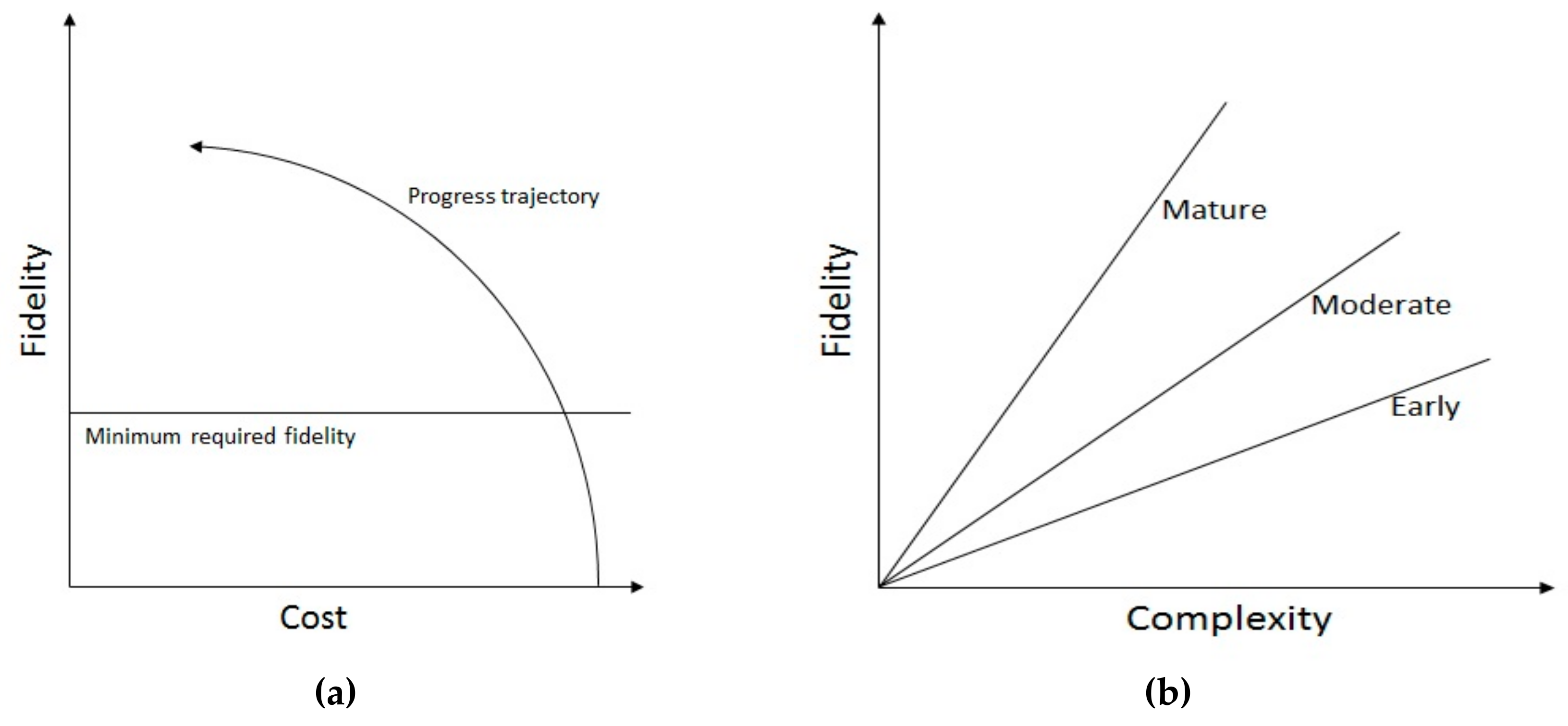
When calculating payoff of M&S, a clear view of the tradeoffs is required to set expectations at reasonable levels, conditioned on the risk behavior of choice: aversion/neutrality/love. Two important tradeoffs are fidelity vs. cost and fidelity vs. complexity. Herein, fidelity refers to the quality of the model in terms of describing the observations and predicting the general behavior of the system for process design and operation relevant scenarios. A typical situation is plotted in Figure 2a,b.
Figure 2a provides a visualization of fidelity vs. cost in the plane where a typical progress trajectory is plotted from conception to optimization vs the minimum level of fidelity required for practical applications. We observe that early efforts in a terra incognita result in high cost and low fidelity. Progressively, one reaches the minimum level of fidelity (though with high cost) but further increases in fidelity eventually lead to cost decline and positive cost-effectiveness balance. Consequently, knowledge of where M&S stands with respect to Figure 2a is imperative for accurate calculations of payoffs.
Figure 2b depicts fidelity vs complexity lines; the lines should be perceived as a first-order approximation of the true relation—in reality, complexity vs. fidelity curves have much more complicated structure. The three lines correspond to early, moderate, and mature M&S in a counter-clockwise fashion. The change in slopes denotes how the accumulation of expertise and know-how leads to leaner approaches; for example, via systematic reductions, symmetry considerations, dimensional arguments, clever discretization techniques etc. Similarly to the fidelity vs cost case, the status quo of fidelity vs complexity should be adequately known.

2.2. Decision Flow-Chart

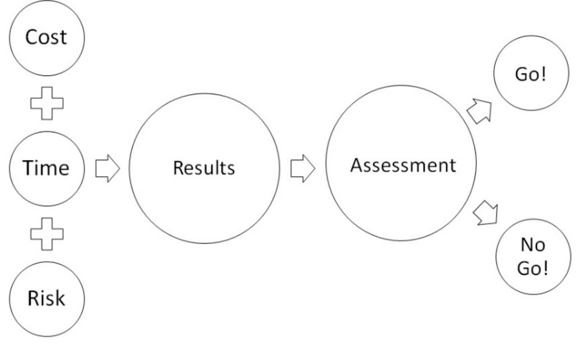
Calculation of payoffs requires an assessment plan of the outcomes of M&S conditioned on the inputs. The flow chart of this process is plotted in Figure 3. We observe that input parameters are cost, time and risk. The output is the results that an M&S exercise yields. It is the assessment of results versus the aggregate effect of cost, time and risk that should drive a go or no go decision for further investment.
For the determination of cost of M&S, we dichotomize models into descriptive and prescriptive ones. Henceforth, A model here is understood as a triplet (governing equations, numerical algorithm/method, software) required for simulation. In other words, it is not only a series of mathematical equations. Descriptive models describe the behavior of existing systems whereas prescriptive models envision to describe the expected behavior of a hypothetical system. For example, a descriptive model would be used to model an existing fermentation vessel. A prescriptive model would be used to design and model a novel fermentation vessel without specific requirements. Descriptive and prescriptive models share similarities with respect to cost, nevertheless, important differences may also be identified. In Table 1, we have tabulated the costs associated with each type of models, further partitioned into upfront (one-time) and recurring costs. One observes the absence of accreditation from prescriptive models; this is to be expected since such models are spearheading R&D and are neither standardized nor subject to systematic upgrades, at least at their early phases of existence. An interesting disparity is the presence of “temptation” in recurring costs. This explains the danger of getting lost in endless exploratory studies, where one goes deeper and deeper whilst there is no clear vision or direction ahead. Cost of temptation may be easy to tame upfront but the lack of a valorization strategy can allow it to skyrocket and undermine budget considerations. Based on Table 1, we can compute the total cost of M&S at year N:
C o s t ( y e a r   N ) = C o s t s o f t + C o s t h a r d + C o s t t r a i n + C o s t s u p g r a d e + # F T E s C o s t F T E
Here, C o s t s o f t and C o s t h a r d designated costs related to procurement of software and hardware whereas C o s t s u p g r a d e stands for maintenance costs and upgrades. C o s t F T E is, as usual, the annual cost of a full-time equivalent while C o s t t r a i n is the cost of related trainings. The concepts of design, implementation, verification, validation, accreditation, and employment are embodied within C o s t F T E . For the sake of simplicity, we have assumed that FTEs in M&S have the same cost.
It is also interesting to visually look at the evolution of cost in time. A linearized picture for both prescriptive and descriptive models is shown in Figure 4. The figure depicts how the temptation point acts as a bifurcation for cost expansion or contraction and how exogenous interventions can act as cost saving mechanisms.
Risk associated with M&S has been well documented. In general, M&S risk comprises (i) accuracy, (ii) descriptive realism, (iii) uncertainty and (iv) applicability; each of these components is defined below:
  • Accuracy is defined as the degree to which the predictions are correct (formally, accuracy is defined with respect to a particular norm.).
  • Descriptive realism refers to the degree that a model predicates upon “true” principles [28].
  • Uncertainty refers to the confidence on outputs, given that some aspects are unknown.
  • Applicability accounting for the potential that the exploitation of the model for the envisioned purpose falls short, because the investigated/modeled phenomena do not govern the system in the a priori expected manner.
Each of these components may be viewed as a normalized function that takes values in the range [0, 1]. For accuracy and descriptive realism, zero and unity denote the minimum and maximum values, respectively and the converse is true for uncertainty. We can therefore define the novel aggregate measure of acceptability according to the following formula:
A c c e p t a b i l i t y = 1 4 ( A c c u r a c y + D e s c r i p t i v e   r e a l i s m + ( 1 u n c e r t a i n t y ) + A p p l i c a b i l i t y )
where L is labor (FTEs + training) and C is physical capital (hardware/software) and a , b are elasticities with a + b < 1 . Acceptability takes values in the range [ 0 ,   1 ] ; an idea M&S exercise would have 1 accuracy, 1 descriptive and 0 uncertainty thus giving acceptability its maximum value: Unity. (One can go a step further and consider a weighted sum of accuracy, descriptive realism and uncertainty. This preferential aggregate would then reflect a heterogeneous prioritization). For practical purposes, acceptability assumes values in the open range (0, 1). Indeed, even at the start of a modeling effort it is unlikely to expect zero acceptability and reaching unity is typically utopic. We take our analysis a step further and link acceptability to cost. To do so, we consider acceptability as an asset and thus the outcome of a production function. To fix ideas, we postulate that the production function follows a Cobb–Douglas form and thus acceptability obeys the following equation:
A c c e p t a b i l i t y = 1 4 ( A c c u r a c y + D e s c r i p t i v e   r e a l i s m + ( 1 u n c e r t a i n t y ) + A p p l i c a b i l i t y ) = L a C b
where L is labor (FTEs + training) and C is physical capital (hardware/software) and a , b are elasticities with a + b < 1 .
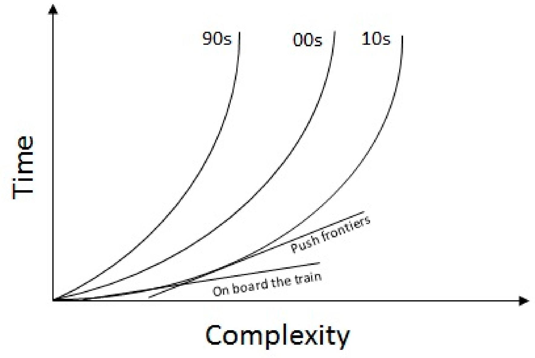
Proponents of M&S typically invoke time as a competitive advantage. However, the required time for M&S depends on the complexity of the problem in hand and the evolving technology and know-how. Figure 5 portrays the trends of time versus complexity for the past decades. As expected, evolution in hardware/software and physical modeling itself pushes the curve in a southeast direction. However, despite this rather robust shift, time remains an exponential function of complexity.
Mathematically, progress increases the part of the curve that can be accurately linearized. This domain is labeled “on board the train” to emphasize that in this area one takes advantage of the accumulated advancements. It is in this zone where time and complexity correlate in a favorable manner. On the right of the “on board the train zone” is the “push the frontiers zone” where a linearized curve changes slope and no longer provides an accurate fit. Here is where innovation mostly occurs. Risk aversion dictates the avoidance of the purely exponential region and the focus on the “push the frontiers” one.
We can further quantify the time required for M&S. Our starting point is the observation that aggregate time required for a M&S exercise can be written as the following sum:
T t o t a l = T m o d e l + T d i g i t i z a t i o n + T s i m u l a t i o n + T i n t e r p r e t a t i o n
where T m o d e l ,   T d i g i t i z a t i o n ,   T s i m u l a t i o n ,   T i n t e r p r e t a t i o n designate the time needed for the development of a model, digitization of equipment, numerical simulation, post-processing and interpretation. An order-of-magnitude analysis can be used to provide some estimates which are reported in Table 2.
We remark that in the case of first time used or newly developed models, T m o d e l accommodates the validation phase as well. Experience has shown that, within pharma, this phase can be quite elongated, as it often involves a chain of actors from non-scientific departments. Thus, one should not underestimate such exogenous factors when drafting (or predicting) time schedules.

3. An Investor’s Approach to M&S

With all the above in mind, we can again call upon our investor, budget owner Mr. X who, correctly or not, has already invested in a M&S team for some time now, being aware of the uncertainty that dominates this decision. Mr. X has now to harvest the results of the investment and needs to define a payoff measure. For a quantitative assessment, Mr. X has to attribute a set of relevant metrics to the corresponding outcomes. This set of metrics will be decomposed into monetary metrics and performance metrics. The need (or rationale) behind this decomposition is as follows. The overall investment has had but a short life and aims in implicitly increasing the net revenue per employee by enhancing the competences that employees have at their disposal. This is not an instantaneous process as Figure 1b asserts. In this respect, Mr. X should keep track not only of monetary payoffs but also of intangible metrics that evaluate the integration of M&S alongside existing R&D practices.

3.1. Monetary Metrics

The first bottleneck is the identification of gains or equivalent the payoff. Three monetary metrics appear as the most prominent candidates: Cost savings, cost avoidance and increased revenues. Formally, they are defined as follows:
  • Cost savings = Cost with M&S—Cost without M&S
  • Cost avoidance = Cost of unnecessary/harmful decision.
  • Increased revenues = profit due to changes in margins or production capacity.
Each of the above monetary metrics can have a single or permanent impact on the sector. Cost savings has a single impact because it refers to gains that do not affect permanently the production capacity and/or revenue. For instance, they may refer to cost savings in a project that failed and never reached production. Cost avoidance has also single impact. It concerns multi-lemmas that once resolved it is for permanent; for example, consider the case where a company needs to decide in favor of one type of instrument vs another. Finally, increased revenues have permanent impact in the corporation. This is a result of M&S permanently affecting the profit margin. (Calculating the above metrics in practice is easier said than done and the typical example is that of knowledge-build projects).
Having collected the required data, Mr. X proceeds to compute a time-dependent return on investment as follows. Consider a time interval [ t 0 , t n ] uniformly discretized into time instances t i such that t i t i 1 = Δ t = c o n s t a n t . Δ t can assume any value, e.g., a month. For each t i calculate the M&S cashflow:
C M S ( t i ) = C o s t   s a v i n g s ( t i t i 1 ) + C o s t   a v o i d a n c e ( t i t i 1 ) + I n c r e a s e d   r e v e n u e s ( t i t i 1 ) I n v e s t m e n t   c o s t ( t i t i 1   )
C o s t   s a v i n g s ( t i t i 1 ) denotes the costs savings during the period t i t i 1 and the same applies for the other components. Consider that C M S ( t i ) have been measured from t 0 = 0 until present t p r e s e n t = K p r e s e n t Δ t . Then, let N p r o j 1 denote the number of projects that M&S personnel have been working on during this time. Each project has an anticipated duration of T j = K j   Δ t , with j = 1 , , N p r o j and T j > t p r e s e n t   j and is expected to induce an internal rate of return (IRR) I R R j , which is a solution to the following;
N P V = i = 0 K j E ( C t o t j ( t i ) ) ( 1 + I R R j ) i = 0
and obeys the following inequality:
I R R j > R R R
In the above relations, E ( C j t o t ( t i ) ) stands for the expectation of the total cash-flow of project j at time instance t i while R R R is the required rate of return which stands for the minimum accepted rate that renders the investment rationally possible. (This is a rather traditional approach. Alternative methodologies that use the real option value such as the Datar–Mathews method, and incorporate risk, may be also utilized) [29].
Next, Mr. X applies a Bayesian inference of the time-series C M S ( t i ) , as duly demonstrated in Figure 6, and calculates stochastic predictions for the evolution of cashflows from t = t p r e s e n t + Δ t until T m a x = max { T j } = K m a x Δ t . Thus, Mr. X obtains a spatio-temporal probability distribution that assigns to each possible C M S ( t i ) a probability. Then, probabilistic estimates of the I R R M S of the M&S investment can be computed according to;
N P V M S = i = 0 K m a x C M S ( t i ) ( 1 + I R R M S ) i = 0 ,   P ( I R R M S ) = p
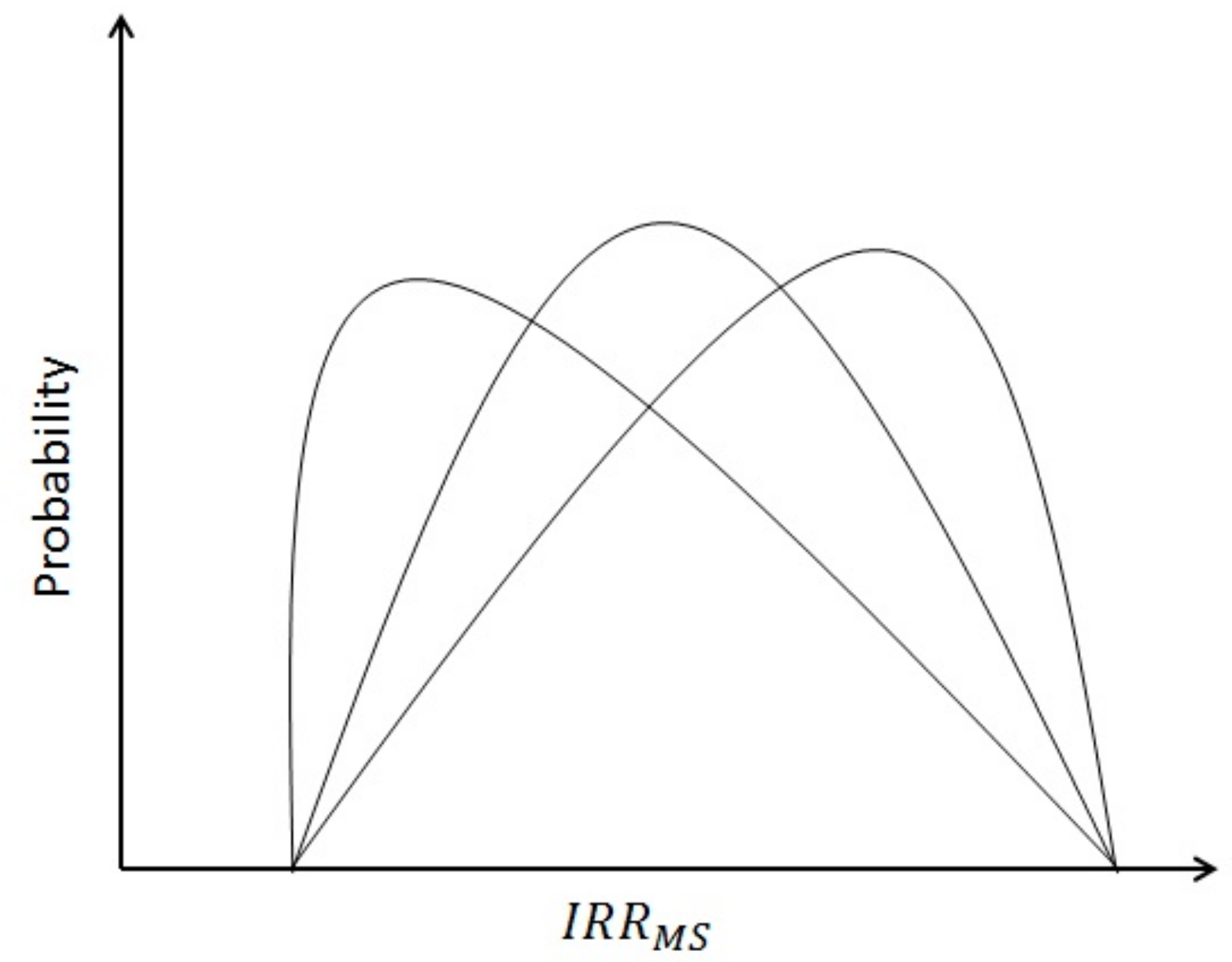
for all possible outcomes enveloped by the Bayesian inference and a graph, like the one reported in Figure 7 displaying predicted I R R M S against probabilities, can be constructed.
Next, a lower limit of acceptance (LLA) for the investment is developed. Assume that I R R M S N ( μ , σ 2 ) . Ostensibly, one could equate LLA with the expected rate of returns R R R . However, we propose a modification so that the degree of diffusion of M&S within the organization is captured. The diffusion of a new technology can be satisfactorily described via a sigmoid function ( t ) = 1 1 + e δ t . (The parameter δ determines the time needed for M&S to completely diffuse, i.e., at which point where the function equals unity. It can be estimated with the help of the intangible metrics of the next section. Other more elaborate and asymmetric functions may also be considered.). Then, a reasonable lower limit of acceptance at time t i is as follows:
L L A ( t i ) = S ( t i ) R R R
We can reconcile the stochastic nature of I R R M S with the risk aversion of Mr. X and Equation (12) as follows. We assign to Mr. X a CARA (constant absolute risk aversion) utility function u ( x ) = 1 e A x with A being the known risk aversion coefficient, that can be estimated via the methodology of [30], and we recall the budget of M $ . Consider the portfolio allocation problem with one risky asset (investment on M&S) with random return I R R M S and a riskless asset with fixed return L L A M S ( T m a x ) . Under rationality, we can explicitly solve this two-asset (one risky and one riskless) portfolio allocation problem, see for example [31]. This solution asserts that that recourses should be allocated if and only if;
μ > L L A M S ( T m a x )
and that the optimal degree of allocation obeys the following condition:
M M S = μ L L A M S ( T m a x ) σ 2 1 A
Equations (13) and (14) have practical implications. First, Mr. X determines whether (13) is satisfied. If yes, then given M 1 $ have already been invested in M&S, Mr. X can solve (14) in terms of the expected return μ , run a sensitivity analysis for σ 2 and end up with a range of values [ μ l o w , μ h i g h ] . Then, Mr. X can compare how well the predictions compare to their realizations, or equivalently where μ lies in the range [ μ l o w , μ h i g h ] .
This is a decision tree with two negative outcomes. First, the realized expected return μ is lower than the lower acceptable limit, i.e., inequality (13) is violated. Thus, the overall investment rates are unfavorable. As the distribution of I R R M S is calculated based on Bayesian inference, it is updated as soon as new data enter the system. Therefore, one should re-evaluate the overall investment at time instances t i > t p r e s e n t and check if violation of inequality (13) is an artifact or not (the generation of monetary gains might come with a (random) time delay). The second negative outcome concerns Equation (14) and the range [ μ l o w , μ h i g h ] . If μ < μ l o w then the investment in M&S is still worthwhile but the expected return is probably overestimated. By contrast, if μ > μ h i g h then the investment outperforms expectations.

3.2. Diffusion-of-Innovation Metrics

Diffusion-of-innovation metrics help our investor, Mr. X, to make better informed decisions when making assessments. The authors of [32] proposed a notoriously high (over 200) number of metrics that constitute assessment criteria of how well modeling and simulation is deployed within the US Department of Defense. Therefore, to a first approximation, this pool of metrics can used for the selection of diffusion-of-innovation metrics that pertain to our case. Of course, it is not only the impractically large number that renders our task challenging but also the fact that several of these metrics are bespoke to the army needs. By merging and redefining available metrics, so as to fit the pharmaceutical world, we have arrived at the following seven (7) performance related metrics, delineated in Table 3 alongside their numerical value.
As the numerical values increase and approach unity so does the integration of M&S in R&D. The numerical values of the metrics s i ,   i = 1 , , 7 are functions of time, i.e., s i = s i ( t j ) where the values t j conform to the previous section discussion. Next, consider the sigmoid function 1 1 + e δ t which has the diffusion rate as a free parameter, δ . Also, consider the sum 1 7 j = 0 K p r e s e n t s i ( t j ) . If the sum of the metrics provides a satisfactory description of the diffusion of M&S in R&D, then it is reasonable to consider the following approximation:
1 1 + e δ t 1 7 j = 0 K p r e s e n t s i t j + u
where u = N ( 0 , σ u 2 ) is a white noise term to reflect the fact that the diffusion process is associated with a certain degree of randomness and can be amenable to random shocks (depending on the strategy that leadership has developed, the diffusion metrics could be assigned a weight ( t j )   with w 1 ( t j ) + w 2 ( t j ) + + w 6 ( t j ) = 1 ; note that the weights are also functions of time to reflect reprioritizations and changes in strategy). Then, the constant δ may be estimated via simple regression from the above equation and directly utilized in Equation (12) of the previous section.

4. Conclusions

Process modeling is gradually gaining momentum within the pharmaceutical industry. This inevitably attracts attention from higher management and onsets the discussion of cost-benefit analysis and investment decisions. This paper has examined process modeling from the investor’s point of view.
We have commenced by examining whether current practices conform to a value-based decision process by using an informed investor as the decision maker. Further, topics like cost, risk and execution time for M&S exercises have also been thoroughly discussed and, wherever possible, mathematical expressions for their description have been introduced. We subsequently proceeded to the development of an easy-to-use methodology that can help an investor evaluate investment on M&S that encompasses both monetary and diffusion-of-innovation based aspects. The proposed methodology builds upon a classical discounted cash flow analysis, infused with elements of Bayesian inference, while accommodating a sigmoid-description of diffusion of innovation for the calculation of lower expected returns. Via the introduction of a set of seven intangible metrics we were also able to quantify the rate with which M&S diffuses within the organization thereby rendering the proposed methodology tractable.
In the present study, we have limited ourselves to the theoretical presentation of the mathematical model were emphasis has been placed on clarifying ideas and concepts. A natural next steps involves exercising the proposed model with either real or simulated data and ideally with both. This step that we intend to pursue as a follow up to this work will play a pivotal role in assessing the predictive capacity of our methodological framework and underlying possible weaknesses that need mitigation.
This concept paper comprises different components that can collectively assist with the difficult task of evaluating M&S. However, herein, we have restricted ourselves to the illustration of these ideas without emphasis on their connectedness. Consequently, a further direction of future research concerns the unification of all ideas presented herein in an umbrella framework.

Author Contributions

C.V., M.v.S., S.D. and A.P. were involved in the design of the study. All authors were involved in drafting the manuscript or critically revising it for important intellectual content. All authors approved the manuscript before it was submitted by the corresponding author.

Funding

This research received no external funding.

Acknowledgments

The authors would like to thank the anonymous reviewers for valuable remarks and suggestions that have substantially improved the quality of the manuscript. Moreover, we thank S. J. E. Evans, N. Giannelos, A. Khan, U. Krause, G. De Lannoy, M. Sanders and M. Vasselle for fruitful discussions and remarks.

Conflicts of Interest

All authors have declared the following interests: All authors are employees of the GSK group of companies. S.D. and A.P. report ownership of shares and/or restricted shares in the GSK group of companies.

References

  1. Petrides, D.P.; Koulouris, A.; Lagonikos, P.T. The Role of Process Simulation in Pharmaceutical Process Development and Product Commercialization. Pharm. Eng. 2002, 22, 56–65. [Google Scholar]
  2. García-Muñoz, S.; Luciani, C.V.; Vaidyaraman, S.; Seibert, K.D. Definition of Design Spaces Using Mechanistic Models and Geometric Projections of Probability Maps. Org. Process Res. Dev. 2015, 19, 1012–1023. [Google Scholar] [CrossRef]
  3. Aboud, L.; Henry, S. New Prescription for Drug Makers: Update the Plants. Leila Aboud & Scott Henry. The Wall Street Journal. 3 September 2003. Available online: https://www.wsj.com/articles/SB10625358403931000 (accessed on 4 September 2019).
  4. Rogers, A.; Ierapetritou, M. Challenges and opportunities in modeling pharmaceutical manufacturing processes. Comput. Chem. Eng. 2015, 81, 32–39. [Google Scholar] [CrossRef]
  5. Muzzio, F.J.; Shinbrot, T.; Glasser, B.J. Powder technology in the pharmaceutical industry: The need to catch up fast. Powder Technol. 2002, 124, 1–7. [Google Scholar] [CrossRef]
  6. McKenzie, P.; Kiang, S.; Tom, J.; Rubin, A.; Futran, M. Can pharmaceutical process development become high tech? AIChE J. 2006, 52, 3990–3994. [Google Scholar] [CrossRef]
  7. Reklaitis, G.V.; Khinast, J.; Muzzio, F. Pharmaceutical engineering science—New approaches to pharmaceutical development and manufacturing. Chem. Eng. Sci. 2010, 65, 4–8. [Google Scholar] [CrossRef]
  8. Eberle, L.G.; Sugiyama, H.; Papadokonstantakis, S.; Graser, A.; Schmidt, R.; Hungerbühler, K. Data-driven Tiered Procedure for Enhancing Yield in Drug Product Manufacturing. Comput. Chem. Eng. 2016, 87, 82–94. [Google Scholar] [CrossRef]
  9. Casola, G.; Siegmund, C.; Mattern, M.; Sugiyama, H. Uncertainty-conscious methodology for process performance assessment in biopharmaceutical drug product manufacturing. AIChE J. 2018, 64, 1272–1284. [Google Scholar] [CrossRef]
  10. Van Bockstal, P.J.; Mortier, S.; De Meyer, L.; Corver, J.; Vervaet, C.; Nopens, I.; De Beer, T. Mechanistic modelling of infrared mediated energy transfer during the primary drying step of a continuous freeze-drying process. Eur. J. Pharm. Biopharm. 2017, 114, 11–21. [Google Scholar] [CrossRef] [Green Version]
  11. Kornecki, M.; Strube, J. Accelerating Biologics Manufacturing by Upstream Process Modelling. Processes 2019, 7, 166. [Google Scholar] [CrossRef]
  12. Metta, N.; Ghijs, M.; Schäfer, E.; Kumar, A.; Cappuyns, P.; Van Assche, I.; Singh, R.; Ramachandran, R.; De Beer, T.; Ierapetritou, M.; et al. Dynamic Flowsheet Model Development and Sensitivity Analysis of a Continuous Pharmaceutical Tablet Manufacturing Process Using the Wet Granulation Route. Processes 2019, 7, 234. [Google Scholar] [CrossRef]
  13. Chatterjee, S.; Moore, C.; Nasr, M. An Overview of the Role of Mathematical Models in Implementation of Quality by Design Paradigm for Drug Development and Manufacture. Food Drug Adm. Papers 2017, 23. [Google Scholar]
  14. Matsunami, K.; Miyano, T.; Arai, H.; Nakagawa, H.; Hirao, M.; Sugiyama, H. Decision support method for the choice between batch and continuous technologies in solid drug product manufacturing. Ind. Eng. Chem. Res. 2018, 57, 9798–9809. [Google Scholar] [CrossRef]
  15. Rantanen, J.; Khinast, J. The Future of Pharmaceutical Manufacturing Sciences. J. Pharm. Sci. 2005, 104, 3612–3638. [Google Scholar] [CrossRef]
  16. Gernaey, K.V.; Woodley, J.; Sin, S. Introducing mechanistic models in Process Analytical Technology education (Research Highlight). Biotechnol. J. 2009, 4, 593–599. [Google Scholar] [CrossRef]
  17. Deloitte Center for Health Solutions. A New Future for R&D? Measuring the Return from Pharmaceutical Innovation; Deloitte Centre for Health Solutions: Deloitte, UK, 2017. [Google Scholar]
  18. DiMasi, J.A.; Hansen, R.W.; Grabowski, H.G. The price of innovation: New estimates of drug development costs. J. Health Econ. 2003, 22, 151–185. [Google Scholar] [CrossRef]
  19. Grabowski, H.; Vernon, J.J. A new look at the returns and risks to pharmaceutical R&D. Manag. Sci. 1990, 36, 804–821. [Google Scholar]
  20. David, E.; Tramontin, T.; Zemmel, R. Pharmaceutical R&D: The road to positive returns. Nat. Rev. Drug Discov. 2009, 8, 609–610. [Google Scholar]
  21. Carter, J., III. A Business Case for Modeling and Simulation; SPECIAL REPORT-RD-AS-01-02; Aviation and Missile Research, Development, and Engineering Center: Redstone Arsenal, AL, USA, 2001. [Google Scholar]
  22. Oswalt, I.; Cooley, T.; Waite, W.; Waite, E.; Gordon, S.; Severinghaus, R.; Feinberg, J.; Lightner, G. Calculating Return on Investment for U.S. Department of Defense Modeling and Simulation; Defense Acquisition Univ. ft. Belvoir VA: Fort Belvoir, VA, USA, 2011. [Google Scholar]
  23. Brown, D.; Grant, G.; Kotchman, D.; Reyenga, R.; Szanto, T. Building a business case for modeling and simulation. Acquis. Rev. Q. 2000, 24, 312–315. [Google Scholar]
  24. Smith, J.M. A Business Case for Using Modeling and Simulation in Developmental Testing; Thesis Naval Postgraduate School; Storming Media: Washington, DC, USA, 2001. [Google Scholar]
  25. Gordon, S.; Oswald, I.; Cooley, T. Why Spend One More Dollar for M&S? Observations on the Return of Investment: Discipline, Ethics, Education, Vocation, Societies, and Economics. In The Profession of Modeling and Simulation; Chapter 14; John Wiley & Sons: Hoboken, NJ, USA, 2017. [Google Scholar]
  26. Glass, H.E.; Kolassa, E.M.; Muniz, E. Drug development through modeling and simulation-The business case. Applied Clinical Trials. 25 July 2016. Available online: http://www.appliedclinicaltrialsonline.com/drug-development-through-modeling-and-simulation-business-case (accessed on 4 September 2019).
  27. Rogers, E. Diffusion of Innovations, 5th ed.; Simon and Schuster: New York, NY, USA, 2003. [Google Scholar]
  28. Meyer, W.J. Concepts of Mathematical Modeling; McGraw-Hill Book Company: New York, NY, USA, 1984. [Google Scholar]
  29. Mathews, S.H.; Datar, V.T.; Johnson, B. A practical method for valuing real options. J. Appl. Corp. Financ. 2007, 19, 95–104. [Google Scholar] [CrossRef]
  30. Babcock, B.A.; Choi, E.K.; Feinerman, E. Risk and probability premiums for CARA utility functions. J. Agric. Resour. Econ. 1993, 18, 17–24. [Google Scholar]
  31. Back, K.E. Asset Pricing and Portfolio Choice Theory; Oxford Univeristy Press: Oxford, UK, 2017. [Google Scholar]
  32. AEgis Technologies Group. Metrics for Modeling and Simulation (M&S) Investments; Naval Air Systems Command Prime Contract No. N61339-05-C-0088; The Aegis Technologies Group, Inc.: Huntsville, AL, USA, 2008. [Google Scholar]
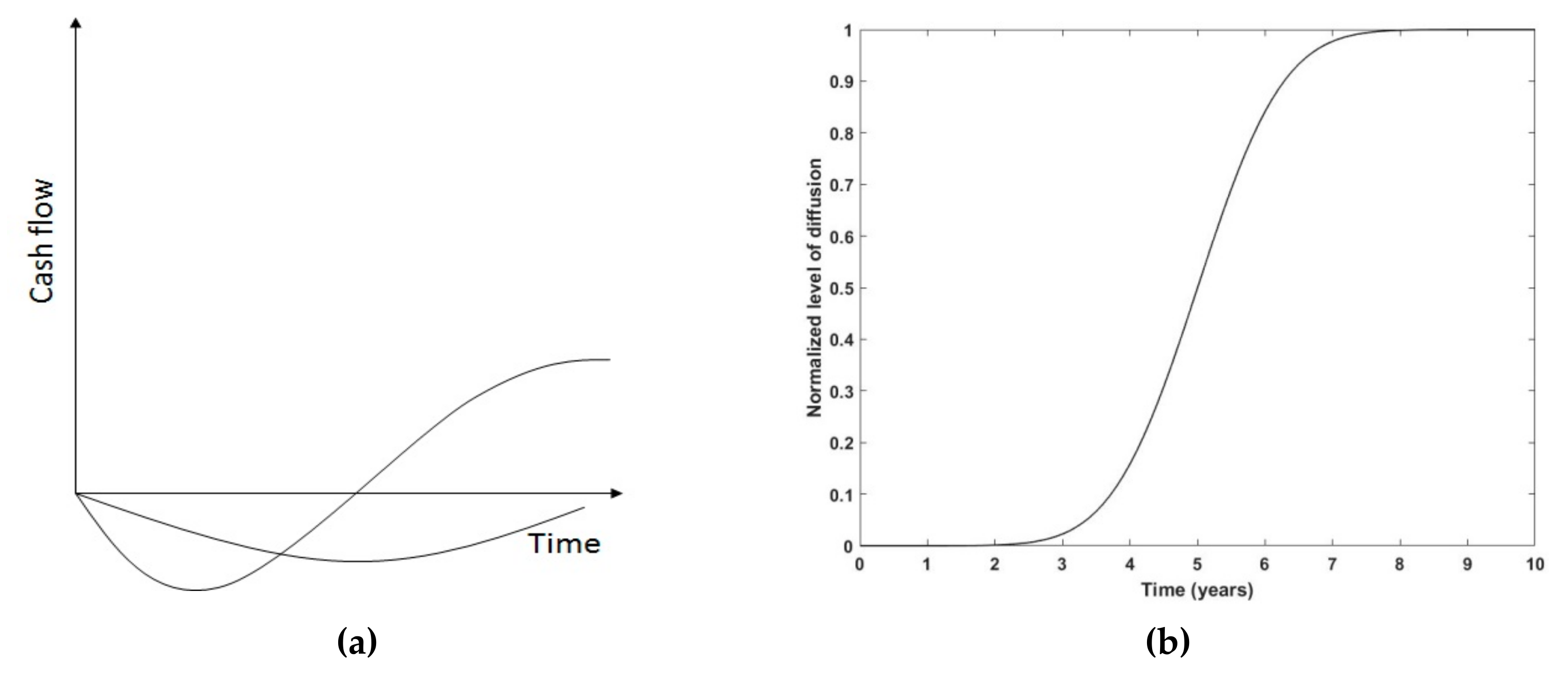
Figure 1. (a) Cash flow of modeling and simulation (M&S) as the time-history of profit, (b) A theoretical Rogers curve for diffusion/penetration of innovation.
Processes 07 00596 g001
Figure 2. (a) Schematic representation of the relationship between fidelity with cost; (b) Schematic representation of fidelity vs complexity.
Processes 07 00596 g002
Figure 3. Flow chart of assessment plan for M&S.
Processes 07 00596 g003
Figure 4. Linearized cost vs. time plots for prescriptive and descriptive models.
Processes 07 00596 g004
Figure 5. Qualitative assessment of required time for M&S. The numbers represent the decades.
Processes 07 00596 g005
Figure 6. Hypothetical data points of C M S ( t i ) vs. time, shown with ∗, concatenated with Bayesian inference.
Processes 07 00596 g006
Figure 7. Predicted I R R M S values vs their probability for three hypothetical cases resulting in three different probability distributions.
Processes 07 00596 g007
Table 1. Cost description for prescriptive and descriptive models.
Upfront CostsRecurring Costs
DescriptiveDesign, Implementation, Verification, Validation, Accreditation, Training, ProcurementEmployment, Upgrades
PrescriptiveDesign, Implementation, Verification, Validation, Training, ProcurementEmployment, Design, Temptation
Table 2. Order-of-magnitude analysis of required time for M&S per component.
Time Required T m o d e l T d i g i t i z a t i o n T s i m u l a t i o n T i n t e r p r e t a t i o n
~DAYSReuseReuseLow & medium complexityNo post-processing required
~WEEKSReuse/discoverDigitize existing systemDetailed CFDMeticulous post-processing/big data
~MONTHSDevelopDesign & digitize systemIndustrial scale CFDN/A
Table 3. Diffusion metrics and their numerical value.
Name of MetricNumerical Value (s)
AwarenessRelative frequency of different projects utilizing M&S
CoordinationRelative frequency of M&S duplicate activities avoided
CongruityRelative frequency of M&S clients correctly interpreting/understanding the results
GuidanceRelative frequency of M&S users conforming to existing standards
ProactivityRelative frequency of (early) decisions made by M&S
EmpowermentRelative frequency of M&S decision makers attending key meetings
FoundationRelative frequency of foundational competencies covered