Maintenance Optimization Model with Sequential Inspection Based on Real-Time Reliability Evaluation for Long-Term Storage Systems

Abstract

For long-term storage systems such as rockets and missiles, most of the relevant models and algorithms for inspection and maintenance currently focus on analysis based on periodic inspection. However, considering factors such as the complexity of the degradation mechanisms of these systems, the constraints imposed by failure risk, and the uncertainty caused by environmental factors, it is preferable to dynamically determine the inspection intervals based on real-time status information. This paper investigates the issue of maintenance optimization modelling for long-term storage systems based on real-time reliability evaluation. First, the Wiener process is used to establish a performance degradation model for one critical unit of such a system, and a closed-form expression for the real-time reliability distribution is obtained by using the first-hitting-time theory. Second, sequential inspection intervals are dynamically determined by combining the real-time reliability function with a real-time reliability threshold for the system. Third, a maintenance optimization model is established for the critical unit based on update process theory. An analytical expression for the expected total cost rate is derived, and then, the real-time reliability threshold and the preventive maintenance threshold for the unit are jointly optimized by means of Monte Carlo simulation, with the lowest expected total cost rate as the optimization goal. Finally, two examples of a gyroscope and an alloy blade that are commonly used in the long-term storage systems are considered, and the validity of the proposed model is illustrated by means of a sensitivity analysis of the relevant parameters.

1. Introduction

“Long-term storage, one-time use” systems, such as missiles and rockets, are kept in long-term storage for the majority of their lifetimes, from the factory to either use or decommissioning, and most such systems are high-value and high-risk products, and thus need to be maintained at a certain level of reliability during this long-term storage. Due to a variety of natural factors (temperature, humidity, gravity, atmospheric pressure, chemical corrosion, etc.) and other induced factors (electromagnetic radiation and static electricity), the components of such a system will gradually degrade in performance, causing some faults. These faults may prevent the product from working properly, resulting in economic losses, and potentially lead to catastrophic accidents. However, in most cases, these faults will be discovered only when a product is required to be put into operation or during an inspection. Thus, if no suitable inspection and maintenance strategy is put into practice, the condition of such products may deteriorate over time, and it will not be possible to eliminate the potential risk in a timely manner. Therefore, it is of great significance to develop an inspection and maintenance optimization model for long-term storage systems.

Three main kinds of inspection schedules are used in condition-based maintenance (CBM): continuous monitoring, periodic inspection, and nonperiodic inspection [1]. The greatest advantage of continuous monitoring is that preventive maintenance can be applied to a system only when necessary, thus reducing wasted inspection and maintenance activities; systems such as nuclear power plants [2], chemical production plants, and aerospace components working under high-stress and high-risk conditions are usually monitored continuously due to the safety risks they pose [3]. To find the optimal degradation thresholds for maintenance intervention for continuously monitored deteriorating systems, Barata and Soares [4] proposed an ‘on condition’ maintenance optimization scheme based on Monte Carlo simulation. A reliability-centered predictive maintenance policy was proposed by Zhou et al. [5] for a continuously monitored system subject to degradation due to imperfect maintenance. Tian et al. [6] also proposed a CBM policy for wind power generation systems in which wind turbine components are monitored continuously. Tang et al. [7] optimized a dynamic CBM policy for a slowly degrading system with real-time condition-monitoring information. Other studies on the development of CBM models for continuously monitored deteriorating systems have also been reported; see the articles of Liao [8], Liu [9] and Besnard [10], for example. While continuous monitoring provides real-time information about the system states, it is always associated with high inspection costs, and errors due to noise typically arise in the many continuous data streams generated in such a scheme. There are also some systems in which continuous monitoring is not applicable. For example, pipelines buried underground, such as those used in the oil and gas industries, cannot be continuously monitored. Another example is the class of long-term storage products studied in this paper, such as rockets and missiles. Due to the complexity, high price and high risk of these systems, it is impossible to carry out continuous power-on inspection. For such systems, only periodic inspections are feasible or affordable. Related optimization models for the inspection interval of a missile under periodic inspection have been extensively studied—see the articles of Shi [11], Fan [12] and Zhang [13], for examples.

Fewer inspections will lead to lower reliability, whereas more frequent inspections will lead to higher costs, both of which are considerable concerns for long-term storage systems; therefore, the optimal inspection policy should establish a suitable trade-off between reliability and operation cost. A nonperiodic inspection policy can lead to potential cost savings since inspections are performed less frequently in the early part of the system lifetime. Hajipour and Taghipour [14] proposed a model for determining the optimal nonperiodic inspection intervals for multicomponent and k-out-of-m systems. An inspection strategy based on a non-fixed period was proposed and applied in precognitive maintenance for monitoring and repair in the context of a multistage degradation process in [15]. Jiang [16] proposed a sequential inspection scheme for determining the state of an item to prevent functional failure, in which the inspection interval and alarm threshold were optimized by means of two cost models. Zhao et al. [17] developed several approximate models for optimal replacement, maintenance, and inspection policies; sequential maintenance policies were also developed to take advantage of their simpler forms, and their optimal solutions were found to be good approximations of the exact policies. Zhu et al. [18] developed a sequential CBM policy for systems subject to stochastic degradation. However, there are currently few nonperiodic inspection strategies for long-term storage systems such as missiles and rockets. Most existing strategies are based on continuous monitoring or periodic inspection, and the optimization of the relevant thresholds is not considered. In addition, the majority of existing CBM research on other products considers either a periodic inspection schedule or a fixed preventive maintenance threshold. To address this gap, this paper focuses on long-term storage systems and proposes corresponding nonperiodic inspection strategies. A sequential inspection policy is used in this paper, and the relevant thresholds are also optimized to improve the efficiency of inspection and maintenance for long-term storage systems.

Various optimization criteria are widely used for CBM, including cost minimization, reliability or availability maximization, and multiobjective optimization. To ensure the normal operation and safety of the products of interest, variations in reliability under different conditions should also be considered. Real-time reliability evaluation is ideal because for dynamic systems, the factors that affect reliability vary continuously with time. Yan [19] developed a two-phase Wiener degradation model to evaluate the real-time reliability of devices. Wang et al. [20] investigated the issue of real-time reliability evaluation based on a general Wiener process-based degradation model. Zhang et al. [21] proposed an effective method and established a framework for real-time reliability assessment based on bridge health monitoring (BHM) acceleration information. In addition, cost is an important factor to consider with regard to the inspection and maintenance process, especially for long-term storage systems, which typically have high inspection and maintenance costs. Guo et al. [22] developed a nonperiodic inspection maintenance model for a single-unit system, in which the preventive maintenance threshold was optimized by minimizing the expected average cost per unit time. Ito et al. [23] optimized the inspection cycles and storage times of long-term storage products in accordance with the different impacts of predetermined maintenance on the failure rate, considering maintenance costs, failure losses and replacement costs, with the lowest average cost rate. Hoseinie [24] considered that in the case of complete maintenance, the minimum maintenance rate can be treated as the optimization goal, and thus obtained the optimal inspection interval for a water injection system. Tan [25] proposed an optimal maintenance strategy for medical instruments with the goal of reducing maintenance costs and improving operational availability. Khatab [26] developed a new maintenance optimization model for failure-prone systems and discussed some of its main cost components; for this model, the preventive maintenance threshold and the number of inspections were optimized separately. In most of the above studies, only one of the variables was optimized, such as the preventive maintenance threshold, the reliability, or the number of inspections. Research on the joint optimization of the real-time reliability threshold and the preventive maintenance threshold has not yet been reported. In addition, to ensure the safety and reliability of a long-term storage system, a reliability constraint value is generally specified first in engineering practice, and the real-time reliability threshold for the long-term storage system during the inspection and maintenance process is included within the specified range of the reliability constraint value. However, it is still uncertain which exact value of the real-time reliability threshold within this range is optimal; consequently, an optimization analysis is needed. Therefore, the real-time reliability threshold and the preventive maintenance threshold should both be decision variables. In our paper, a maintenance optimization model based on minimizing the expected total cost rate is established. Thus, we can not only ensure high reliability and safety of the long-term storage system but also reduce the costs of inspection and maintenance.

In this paper, we propose a maintenance optimization model for a long-term storage system under sequential inspection. The objective of the optimization model is to jointly find the optimal real-time reliability threshold and the optimal preventive maintenance threshold such that the expected total cost rate over an infinite time span is minimized. The model proposed in this paper can make full use of the mathematical properties of the Wiener process, and the uncertainty of stochastic model parameter estimation is also considered. Thus, the random degradation processes of key long-term storage units can be well fitted, and an expression for the real-time reliability of such a unit is derived. This expression is combined with the real-time reliability threshold to determine a sequential inspection policy for such a long-term storage system. In addition, based on update process theory and the real-time reliability model, a maintenance optimization model for a critical unit subjected to sequential inspection is given, where the minimum expected total cost rate is taken as the optimization goal, and an analytical expression for the expected total cost rate is also derived. Then, the optimal values of the real-time reliability threshold and the preventive maintenance threshold can be obtained by means of Monte Carlo simulation. The model proposed in this paper not only can guarantee the safety and reliability of a long-term storage system but also can improve the efficiency of inspection and maintenance and reduce maintenance costs, thus providing decision-making support for the development of inspection and maintenance strategies for long-term storage systems.

The remainder of this paper is organized as follows. In Section 2, we specify some assumptions and present the flow chart of the proposed methodology. In Section 3, we introduce the specific method of real-time reliability evaluation. In Section 4, we propose a sequential inspection model and discuss the maintenance strategy. Then, we establish the maintenance optimization model in Section 5. In Section 6, we present two examples to validate the model proposed in this paper. Finally, we conclude our work in Section 7.

2. Assumptions and Methodology

The long storage system is a complex system, composed of a variety of components, devices and subsystems. Taking the missile system as an example, it is mainly composed of four parts: warhead, power device, guidance system, and missile body structure. The research object in this paper refers to the key units that have important influence on the long storage system, which can be the key component, such as the alloy blade of the rocket engine, or the key device in the subsystem, such as the gyroscope in the guidance system. Therefore, the unit in this paper can be either a single component, a single device or a single subsystem.

The Wiener process has been widely used by researchers to describe the degradation of aviation units, such as satellite momentum wheels, rocket engine blades, and gyroscopes. The Wiener process can be used to describe not only nonmonotonic degradation processes but also monotonic degradation processes, making it an important tool for describing the degradation of units’ performance.

2.1. Assumptions of The Degradation Model

(1) Each critical unit of the system of interest is a degraded component, and its degradation process can be described by a smooth Wiener process subject to the following conditions.

• If $t=0$, the degradation level of the unit is 0, i.e., $X\left(0\right)=0$, and the unit is in the normal state.
• The degradation increments ($X\left(t_j\right)-X\left(t_i\right)$) of the unit in different time intervals $\left(t_i,t_j\right)$ are independent of each other and obey a normal distribution: $X\left(t_j\right)-X\left(t_i\right)~N\left(\mu \left(t_j-t_i\right),{\sigma }^2\left(t_j-t_i\right)\right)$

(2) When the degradation state of a critical unit reaches its failure threshold $w(w>0)$, the resulting component failure will cause system failure. The failure time is defined based on the first-hitting-time theory for a random process, i.e., $T_f=\inf \{t:X\left(t\right)\ge w|X\left(t_i\right)\}$. Here, $w$ is a fixed value that is set in accordance with various constraints, such as those arising from engineering experience and design requirements. $w_0(0<w_0<w)$ is the threshold for preventive maintenance, which can be adjusted based on the requirements of the maintenance strategy.

(3) In engineering practice, a reliability constraint $R^{*}$ is generally specified first for each critical unit of a long-term storage system to ensure its safety and reliability. In other words, the evaluated real-time reliability $q$ of each critical unit must be no less than $R^{*}$; otherwise, the required reliability constraint will not be met.

(4) Due to cost constraints and the limitations of the inspection method, the state of a critical unit cannot be monitored in real-time; instead, the degradation information of the unit can be obtained only by means of noncontinuous inspection. It is further assumed that there are no errors in the inspection results.

(5) The time required for the inspection, repair or replacement of a critical unit is assumed to be negligible in comparison to the long-term storage cycle of the system.

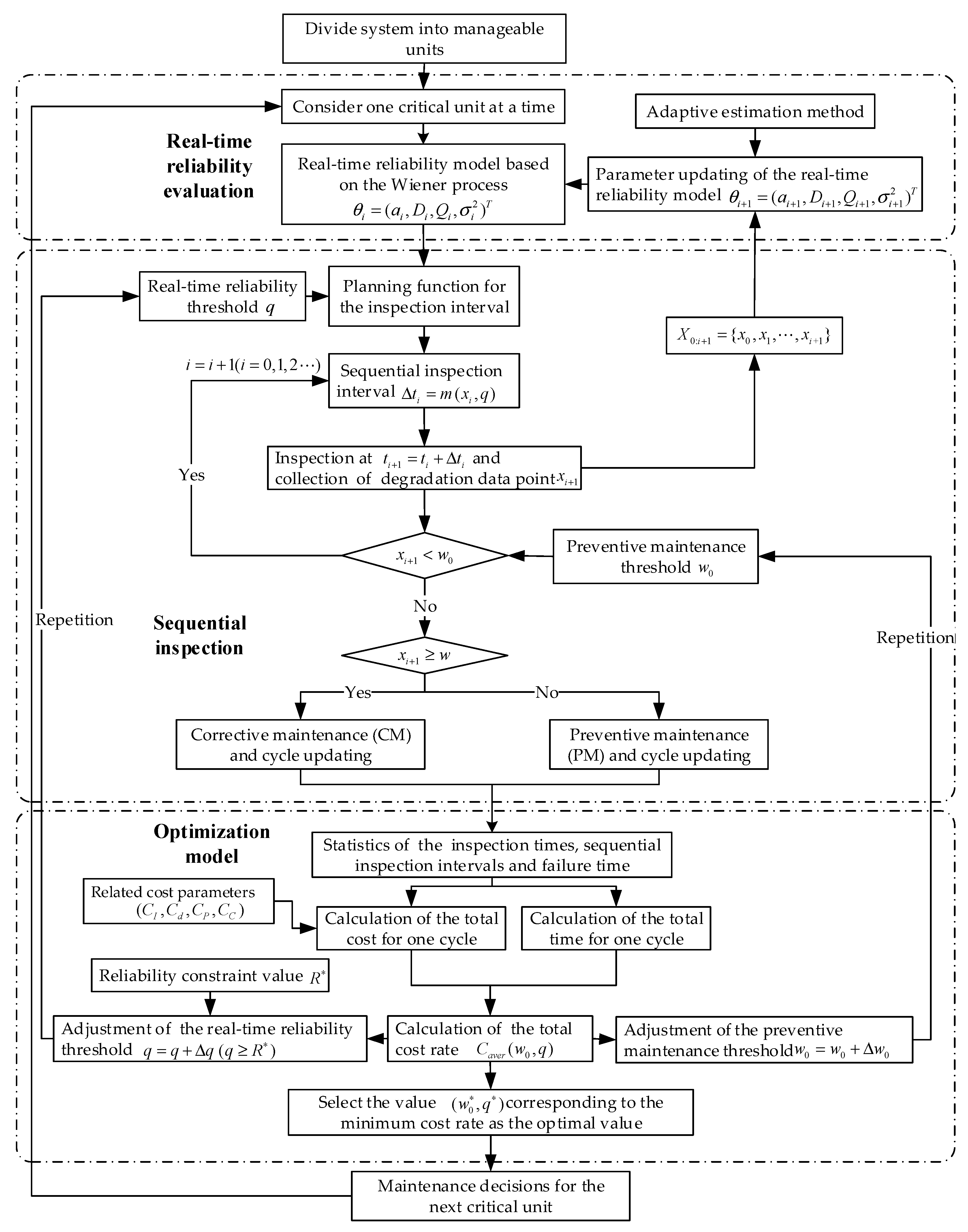
2.2. Maintenance and Optimization Methodology

The proposed methodology is broken down into three main modules (see Figure 1):

(1)

Real-time reliability evaluation, which mainly consists of establishing the real-time reliability model and adaptively updating the parameters.

(2)

Sequential inspection, which mainly consists of determining the inspection intervals and making maintenance decisions (preventive maintenance or corrective maintenance).

(3)

Optimization model, which mainly consists of establishing the cost model and calculating the optimal values.

3. Real-Time Reliability Evaluation

For certain critical units of a system that is in long-term storage, their reliability needs to be evaluated to enable relevant maintenance decisions. If such a critical unit has not failed at the current time, a conditional probability can be used to represent its level of reliability. When a new degradation data point is obtained, this real-time reliability can be updated.

On the basis of the first-hitting-time theory of random processes, Wang [27] investigated the issue of real-time reliability evaluation based on a general Wiener process-based degradation model. Accordingly, we can use Equation (1) to measure the real-time reliability of a critical unit:

$$R\left(t;X_{0:k},{\theta }_k\right)=P(X\left(\tau \right)<w,\forall \tau \in \left[t_k,t\right]|{\theta }_k,X_{0:k},X\left(t_j\right)<w,j=1,2,\cdots ,k)$$

(1)

where ${\theta }_k={\left(a_k,D_k,Q_k,{\sigma }_k{}^2\right)}^T$ and $X_{0:k}$ is the set of degradation data $\{x_0,x_1,\cdots x_k\}$, with $X\left(t_k\right)=x_k$ being the degradation data point for the unit at inspection time $t_k$. In this study, the random drift parameter $\mu$ is defined in accordance with a random walk model as described by Si [28]; this parameter can be updated as new inspection data are obtained, i.e., ${\mu }_k={\mu }_{k-1}+\eta$, where $\eta \sim N\left(0,Q\right)$ and ${\mu }_k\sim N\left(a_k,D_k\right)$. Therefore, the drift coefficient $\mu$ is a random variable that varies with time and depends on the value ${\mu }_{k-1}$ at the previous moment; the diffusion coefficient in the Wiener process is ${\sigma }_k$. To obtain the expression for $R\left(t;X_{0:k},{\theta }_k\right)$, the remaining life of the product is first defined as follows

$$L_k=\inf \{l_k:X\left(l_k+t_k\right)\ge w|X_{0:k},X\left(t_j\right)<w,j=1,2,\cdots ,k\}$$

(2)

Thus, $R(t,X_{0:k},{\mathbf{\theta }}_k)$ can be expressed as follows

$$R\left(t;X_{0:k},{\theta }_k\right)=P(L_k>t-t_k)$$

(3)

Similarly, the probability density function (PDF) for the remaining life of the product can be obtained using the following formula [28].

$$f_{T|x_k}(t|x_k)=\frac{w-x_k}{\sqrt{2\pi {(t-t_k)}^3{\sigma }^2}}exp\{-\frac{{(w-x_k-\mu \left(t-t_k\right))}^2}{2{\sigma }^2\left(t-t_k\right)}\}$$

(4)

Then, for an inspection interval of $t-t_k=\Delta t_k$, the real-time reliability of the product can be obtained as follows

$$\begin{array}{l}{R}_S(\Delta t_k|X_{0:k})={{\displaystyle \int }}_{t-t_k}^{\infty }{f}_{L_k|X_{0:k}}(l_k|X_{0:k})d{l}_k={{\displaystyle \int }}_{\Delta t_k}^{\infty }{f}_{L_k|X_{0:k}}(l_k|X_{0:k})d{l}_k\\ =\Phi \left(\frac{w-x_k-{\widehat{\mu }}_k\Delta t_k}{\sqrt{D_k\Delta t_k{}^2+{\sigma }_k^2\Delta t_k}}\right)-exp\left\{\frac{2{\widehat{\mu }}_k\left(w-x_k\right)}{{\sigma }_k^2}+\frac{2D_k{(w-x_k)}^2}{{\sigma }_k^4}\right\}\\ \times \Phi \left(-\frac{2D_k\left(w-x_k\right)\Delta t_k+{\sigma }_k^2\left({\widehat{\mu }}_k\Delta t_k+w-x_k\right)}{{\sigma }_k^2\sqrt{D_k\Delta t_k{}^2+{\sigma }_k^2\Delta t_k}}\right)\end{array}$$

(5)

In Equations (3) and (5), $a_k$, $D_k$, $Q_k$, and ${\sigma }_k^2$ are unknown parameters of the random degradation model, which need to be estimated based on the inspection data $X_{0:k}$. Based on the adaptive estimation method presented in [29], which combines the strong tracking filtering algorithm, the Rauch–Tung–Striebel (RTS) smoothing algorithm, and the expectation maximization (EM) algorithm, the parameter estimates ${\widehat{\theta }}_k=(a_{0k}^{\left(i+1\right)},D_{0k}^{\left(i+1\right)},Q_k^{\left(i+1\right)},({\sigma }^2{)}_k^{\left(i+1\right)})$ can be adaptively updated based on the degradation data $X_{0:k}$ obtained from the inspection process.

4. Sequential Inspection and Maintenance Strategy

A long-term storage system will undergo a series of inspections $I=\{t_1,t_2,\cdots ,t_n\}$ during its life cycle, where $t_i\in I$ is the time of the i-th inspection, and will eventually be subjected to either preventive maintenance (PM) or corrective maintenance (CM). At each inspection time, it is necessary to decide which maintenance activities are to be performed based on the current state of the system. If maintenance is not required, the next inspection interval should be determined.

4.1. Sequential Inspection Intervals

In engineering practice, a reliability constraint value $R^{*}$ is generally set for each critical unit to ensure the safety and reliability of a system during long-term storage. Therefore, if $q$ denotes the real-time reliability threshold of the unit, the condition $q\ge R^{*}$ must be met.

For a critical unit in a long-term storage system, the i-th inspection time is denoted by $t_i\left(i=1,2,\cdots \right)$, the initial time is $t_0=0$, and the degradation level of the component at time $t_i$ is denoted by $X\left(t_i\right)=x_i$. According to Equation (5) in Section 3, which gives the expression for the real-time reliability function, the next inspection time for the system can be expressed as follows

$$t_{i+1}=t_i+\Delta t_i=t_i+m\left(X\left(t_i\right),q\right)=t_i+m\left(x_i,q\right)$$

(6)

where $m\left(X\left(t_i\right),q\right)$ is the planning function for the inspection time, which consists of the real-time reliability function, the real-time reliability threshold $q$ and the degradation data point $X\left(t_i\right)$. $\Delta t_i$ is the result calculated using the planning function $m\left(X\left(t_i\right),q\right)$ and represents the time interval between the i-th inspection and the (i + 1)-th inspection.

In Section 3, the expression for the real-time reliability has been obtained; based on this expression, the inspection time planning function $m\left(X\left(t_i\right),q\right)$ can be expressed as follows

$$\begin{gathered} \begin{array}{l}{R}_S(m\left(X\left(t_i\right),q\right)|X_{0:i})=R_S(\Delta t_i|X_{0:i})\\ \\ =\Phi \left(\frac{w-x_i-{\widehat{\mu }}_i\Delta t_i}{\sqrt{D_i\Delta t_i{}^2+{\sigma }_i^2\Delta t_i}}\right)-exp\left\{\frac{2{\widehat{\mu }}_i\left(w-x_i\right)}{{\sigma }_i^2}+\frac{2D_i{(w-x_i)}^2}{{\sigma }_i^4}\right\}\times \end{array} \\ \Phi \left(-\frac{2D_i\left(w-x_i\right)\Delta t_i+{\sigma }_i^2\left({\widehat{\mu }}_i\Delta t_i+w-x_i\right)}{{\sigma }_i^2\sqrt{D_i\Delta t_i{}^2+{\sigma }_i^2\Delta t_i}}\right)=q\left(q\ge R^{*}\right) \end{gathered}$$

(7)

Based on the real-time reliability threshold $q$, the inspection time planning function $m\left(X\left(t_i\right),q\right)$ can be solved to obtain the inspection interval $\Delta t_i$.

4.2. Maintenance Strategy

The performance degradation and maintenance process of a critical unit under sequential inspection is shown in Figure 2, where $H_i\left(i=1,2\cdots \right)$ represents the length of the i-th update cycle.

As seen in Figure 2, the unit is sequentially inspected, with the next inspection interval being determined at the time of the current inspection, and a relevant maintenance strategy can be further developed based on the obtained degradation information. The related maintenance strategies are as follows.

(1)

If the degradation state of the unit when it is inspected at time $t_i$ is $x_i<w_0$, the system will continue to be stored without maintenance, and the next inspection time $t_{i+1}$ will be determined in accordance with the current degradation level $x_i$ and the inspection time planning function. The cost of each inspection is denoted by $C_I$, and $w_0$ is a PM threshold that can be optimized.

(2)

The real-time reliability threshold $q$ has an important impact on the inspection and maintenance cost; therefore, it is also a value that can be optimized.

(3)

If $w_0\le x_i<w$, PM will be performed on the unit. After PM, the performance state of the unit will be restored to the same level as when the unit was new, the degradation level will also return to the initial state, and the update cycle of the system will be recalculated from 0, i.e., $X\left(0\right)=0$. The cost of each instance of PM is denoted by $C_P$.

(4)

If $x_i\ge w$, meaning that the degradation level exceeds the failure threshold, CM must be performed on the unit. Similarly to the case of PM, after CM, the unit will be restored to like-new performance, the degradation level will also return to the initial state, and the system cycle will be recalculated from 0. The cost of each instance of CM is denoted by $C_C$.

(5)

If $x_{i-1}<w_0$ and $x_i\ge w$, the system will be in a faulty state for a certain period of time before CM can be performed; the length of this period is denoted by $d\left(t\right)$, and $C_d$ is the cost of failure loss per unit time.

(6)

The relationship between the costs of inspection, maintenance and failure loss satisfies $C_I<C_d<C_P<C_C$.

5. Maintenance Optimization Model

The maintenance optimization model established in this paper attempts to achieve the minimum maintenance cost rate under long-term storage. An analytical expression for the expected total cost rate is derived based on update process theory. Then, Monte Carlo simulations are used to obtain the optimal values of two decision variables, namely, the optimal PM threshold $w_0^{*}$ and the optimal real-time reliability threshold $q^{*}$.

5.1. Expected Cost Rate Model

According to update process theory [30], the expected cost rate for a system under long-term storage can be estimated based on the expected cost rate for one update cycle. Based on the maintenance strategy described above, the inspection and maintenance cost for the system during one update cycle H can be expressed as follows

$$\begin{gathered} C\left(H\right)={\displaystyle \sum }_{j=1}^{\infty }\left(j{C}_I+C_P\right)I_{\{x_{j-1}<w_0\le x_j<w\}} \\ +{\displaystyle \sum }_{j=1}^{\infty }(j{C}_I+C_C+C_d{{\displaystyle \int }}_{t_{j-1}}^{t_j}\left(t_j-t\right)d{F}_{\mu ,\sigma }(t))I_{\{x_{j-1}<w_0,x_j\ge w\}} \end{gathered}$$

(8)

Here, $I_{\{·\}}$ is an indicative function such that $I_{\{·\}}=1$ when the condition in $\{·\}$ is satisfied and $I_{\{·\}}=0$ otherwise. $F_{\mu ,\sigma }\left(t\right)$ is the lifetime distribution function of the critical unit of interest based on the Wiener process, namely,

$$\begin{gathered} \begin{array}{ll}{F}_{\mu ,\sigma }\left(t\right)={{\displaystyle \int }}_w^{\infty }{f}_{\mu ,\sigma }& (x)dx\\ & =\Phi \left(\frac{\mu t-w}{\sqrt{D{t}^2+{\sigma }^{2}t}}\right)\\ & +exp\left(\frac{2\mu w}{{\sigma }^2}+\frac{2D{w}^2}{{\sigma }^4}\right)\Phi \left(-\frac{2Dwt+{\sigma }^2\left(\mu t+w\right)}{{\sigma }^2\sqrt{D{t}^2+{\sigma }^{2}t}}\right)\end{array} \\ {f}_{\mu ,\sigma }\left(t\right)=\frac{w}{\sqrt{2\pi t^3\left(Dt+{\sigma }^2\right)}}exp\left[-\frac{{(w-\mu t)}^2}{2\left(Dt+{\sigma }^2\right)t}\right] \end{gathered}$$

(9)

Note that $\mu$ and $\sigma$ are parameters that are updated in real-time following the real-time reliability evaluation procedure presented in Section 3, and the parameters from the previous inspection are used to evaluate the time at which the degradation level of the unit is expected to reach the failure threshold.

The length of the system’s update cycle H is

$$T\left(H\right)={\displaystyle \sum }_{j=1}^n{t}_j{I}_{\{x_{j-1}<w_0\le x_j<w\}}+{\displaystyle \sum }_{j=1}^n{t}_j{I}_{\{x_{j-1}<w_0,x_j\ge w\}}$$

(10)

According to update process theory [30], the long-term expected total cost per unit time can be calculated using the expected total cost rate for one update cycle H. Based on this approach, the expected total cost rate $C_{aver}(w_0,q)$ is

$$C_{aver}\left(w_0,q\right)=\underset{t\to \infty }{lim}E\left[\frac{C\left(t\right)}{t}\right]=\frac{E\left[C\left(H\right)\right]}{E\left[T\left(H\right)\right]}$$

(11)

where $C(t)$ is the total cost for the inspection and maintenance of the unit over a time period $t$.

To calculate Equation (11), the expected values of Equations (8) and (10) need to be calculated first. $P_P(j)$ and $P_C(j)$ denote the probabilities of PM and CM, respectively, after the j-th inspection of the unit, namely,

$$P_P\left(j\right)=P(x_{j-1}<w_0\le x_j<w)$$

(12)

$$P_C\left(j\right)=P(x_{j-1}<w_0,x_j\ge w)$$

(13)

(1) When $j=1$, the first inspection interval $\Delta t_0$ can be obtained according to the inspection planning function given in Equation (7) and the approximate initial parameters ${\theta }_0={\left(a_0,D_0,Q_0,{\sigma }_0{}^2\right)}^T$, yielding the following Equations.

$$\begin{array}{l}{R}_S(m\left(x_0,q\right)|x_0)=R_S(\Delta t_0|x_0)\\ =\Phi \left(\frac{w-x_0-{\widehat{\mu }}_0\Delta t_0}{\sqrt{D_0\Delta t_0{}^2+{\sigma }_0^2\Delta t_0}}\right)-exp\{\frac{2{\widehat{\mu }}_0\left(w-x_0\right)}{{\sigma }_0^2}+\frac{2D_0{(w-x_0)}^2}{{\sigma }_0^4}\}\times \\ \Phi \left(-\frac{2D_0\left(w-x_0\right)\Delta t_0+{\sigma }_0^2\left({\widehat{\mu }}_0\Delta t_0+w-x_0\right)}{{\sigma }_i^2\sqrt{D_i\Delta t_0{}^2+{\sigma }_0^2\Delta t_0}}\right)=q\left(q\ge R^{*}\right)\end{array}$$

(14)

$$t_1=t_0+\Delta t_0\left(t_0=0\right)$$

(15)

In addition, the degradation data point $x_1$ for the same unit at the first inspection can be similarly obtained according to the approximate initial parameters ${\theta }_0={\left(a_0,D_0,Q_0,{\sigma }_0{}^2\right)}^T$:

$$\begin{gathered} x_1=x_0+\Delta x_0\left(x_0=0\right) \\ \Delta x_0~N\left({\mu }_0\Delta t_0,{\sigma }_0^2\Delta t_0\right) \end{gathered}$$

(16)

Then, we can obtain $P_P(1)$ and $P_C(1)$ as follows

$$P_P\left(1\right)=P(w_0\le x_1<w)=F_{{\mu }_0,{\sigma }_0}\left(\Delta t_0;w_0\right)-F_{{\mu }_0,{\sigma }_0}\left(\Delta t_0;w\right)$$

(17)

$$P_C\left(1\right)=P\left(x_1\ge w\right)=F_{{\mu }_0,{\sigma }_0}\left(\Delta t_0;w\right)$$

(18)

where

$$\begin{array}{l}{F}_{{\mu }_0,{\sigma }_0}\left(\Delta t_0;w\right)=\Phi \left(\frac{{\mu }_0\Delta t_0-w}{\sqrt{D_0\Delta t_0{}^2+{\sigma }_0^2\Delta t_0}}\right)+\\ exp\left(\frac{2{\mu }_{0}w}{{\sigma }_0^2}+\frac{2D_0{w}^2}{{\sigma }_0^4}\right)\Phi \left(-\frac{2D_{0}w\Delta t_0+{\sigma }_0^2\left({\mu }_0\Delta t_0+w\right)}{{\sigma }_0^2\sqrt{D_0\Delta t_0{}^2+{\sigma }_0^2\Delta t_0)}}\right)\end{array}$$

(19)

(2) When $j\ge 2$, first, the degradation data points $\{x_0,x_1,\cdots x_{j-1}\}$ are used to update the model parameters ${\theta }_{j-1}={(a_{j-1},D_{j-1},Q_{j-1},{\sigma }_{j-1}^2)}^T$ by means of the adaptive estimation method presented in [29]. Then, the j-th inspection interval $\Delta t_{j-1}$ can be determined in accordance with the inspection time planning function:

$$\begin{array}{l}{R}_S(m\left(x_{j-1},q\right)|X_{0:j-1})=R_S(\Delta t_{j-1}|X_{0:j-1})\\ =\Phi \left(\frac{w-x_{j-1}-{\widehat{\mu }}_{j-1}\Delta t_{j-1}}{\sqrt{D_{j-1}\Delta t_{j-1}{}^2+{\sigma }_{j-1}^2\Delta t_{j-1}}}\right)-exp\{\frac{2{\widehat{\mu }}_{j-1}\left(w-x_{j-1}\right)}{{\sigma }_{j-1}^2}+\frac{2D_{j-1}{(w-x_{j-1})}^2}{{\sigma }_1^4}\}\times \\ \Phi \left(-\frac{2D_{j-1}\left(w-x_{j-1}\right)\Delta t_{j-1}+{\sigma }_{j-1}^2\left({\widehat{\mu }}_{j-1}\Delta t_{j-1}+w-x_{j-1}\right)}{{\sigma }_{j-1}^2\sqrt{D_{j-1}\Delta t_{j-1}{}^2+{\sigma }_{j-1}^2\Delta t_{j-1}}}\right)=q\left(q\ge R^{*}\right)\end{array}$$

(20)

Thus, the j-th inspection time $t_j$ is as follows

$$t_j=t_{j-1}+\Delta t_{j-1}={\displaystyle \sum }_{n=1}^j\Delta t_{n-1}\left(j\ge 2\right)$$

(21)

Similarly, the degradation data point $x_j$ collected at the j-th inspection can be obtained in accordance with the parameters ${\theta }_{j-1}={(a_{j-1},D_{j-1},Q_{j-1},{\sigma }_{j-1}^2)}^T$:

$$\begin{array}{l}{x}_j=x_{j-1}+\Delta x_{j-1}=x_0+{\displaystyle \sum _{n=1}^j}\Delta x_{n-1}\left(j\ge 2\right)\\ \Delta x_0~N\left({\mu }_0\Delta t_0,{\sigma }_0^2\Delta t_0\right)\\ \Delta x_1~N\left({\mu }_1\Delta t_1,{\sigma }_1^2\Delta t_1\right)\\ \cdots \cdots \\ \Delta x_{n-1}~N\left({\mu }_{n-1}\Delta t_{n-1},{\sigma }_{n-1}^2\Delta t_{n-1}\right)\end{array}$$

(22)

Then, we can obtain $P_P\left(j\right)$ and $P_C\left(j\right)$ as follows

$$\begin{array}{l}{P}_P\left(j\right)=P(x_{j-1}<w_0\le x_j<w)\\ =P(x_{j-1}<w_0,w_0-x_{j-1}\le x_j-x_{j-1}<w-x_{j-1})\\ ={{\displaystyle \int }}_0^{w_0}{f}_{\varphi \left({\mu }_{j-1},{\sigma }_{j-1}\right)}\left(x;t_{j-1}\right)(F_{{\mu }_{j-1},{\sigma }_{j-1}}\left(\Delta t_{j-1};w_0-x\right)-F_{{\mu }_{j-1},{\sigma }_{j-1}}\left(\Delta t_{j-1};w-x\right))dx\end{array}$$

(23)

$$\begin{array}{l}{P}_C\left(j\right)=P(x_{j-1}<w_0,x_j\ge w)=P(x_{j-1}<w_0,x_j-x_{j-1}\ge w-x_{j-1})\\ ={{\displaystyle \int }}_0^{w_0}{f}_{\varphi \left({\mu }_{j-1},{\sigma }_{j-1}\right)}\left(x;t_{j-1}\right)F_{{\mu }_{j-1},{\sigma }_{j-1}}\left(\Delta t_{j-1};w-x\right)dx\end{array}$$

(24)

where $f_{\varphi \left({\mu }_{j-1},{\sigma }_{j-1}\right)}\left(x;t_{j-1}\right)$ represents the PDF of the unit when the degradation level is $x$ at time $t_{j-1}$ based on the Wiener process, namely,

$$f_{\varphi \left({\mu }_{j-1},{\sigma }_{j-1}\right)}\left(x;t_{j-1}\right)=\frac{1}{\sqrt{2\pi t_{j-1}\left({\sigma }_{j-1}^2+D_{j-1}{t}_{j-1}\right)}}\times exp\left[-\frac{{(x-{\mu }_{j-1}{t}_{j-1})}^2}{2\left({\sigma }_{j-1}^2+D_{j-1}{t}_{j-1}\right)t_{j-1}}\right]$$

(25)

$$\begin{array}{l}{F}_{{\mu }_{j-1},{\sigma }_{j-1}}\left(\Delta t_{j-1};w-x\right)\\ =\Phi \left(\frac{{\mu }_{j-1}\Delta t_{j-1}-\left(w-x\right)}{\sqrt{D_{j-1}\Delta t_{j-1}{}^2+{\sigma }_{j-1}^2\Delta t_{j-1}}}\right)+exp\left(\frac{2{\mu }_{j-1}\left(w-x\right)}{{\sigma }_{j-1}^2}+\frac{2D_{j-1}{(w-x)}^2}{{\sigma }_{j-1}^4}\right)\times \\ \Phi \left(-\frac{2D_{j-1}\left(w-x\right)\Delta t_{j-1}+{\sigma }_{j-1}^2\left({\mu }_{j-1}\Delta t_{j-1}+w-x\right)}{{\sigma }_{j-1}^2\sqrt{D_{j-1}\Delta t_{j-1}{}^2+{\sigma }_{j-1}^2\Delta t_{j-1}}}\right)\end{array}$$

(26)

Based on Equations (14)–(26), the expected total cost for the inspection and maintenance of the unit during one update cycle can be obtained as follows

$$\begin{array}{l}E\left[C\left(H\right)\right]={\displaystyle \sum _{j=1}^{\infty }}\left(j{C}_I+C_P\right)P_P\left(j\right)+{\displaystyle \sum _{j=1}^{\infty }}(j{C}_I+C_C+C_d{{\displaystyle \int }}_{t_{j-1}}^{t_j}\left(t_j-t\right)d{F}_{\mu ,\sigma }\left(t\right))P_C\left(j\right)\\ =\left(C_I+C_P\right)P_P\left(1\right)+(C_I+C_C+C_d{{\displaystyle \int }}_0^{\Delta t_0}\left(\Delta t_0-t\right)d{F}_{{\mu }_0,{\sigma }_0}\left(t\right))P_C\left(1\right)+\\ {\displaystyle \sum _{j=2}^{\infty }}\left(j{C}_I+C_P\right)P_P\left(j\right)+{\displaystyle \sum _{j=2}^{\infty }}(j{C}_I+C_C+C_d{{\displaystyle \int }}_{t_{j-1}}^{t_j}\left(t_j-t\right)d{F}_{{\mu }_{j-1},{\sigma }_{j-1}}\left(t\right))P_C\left(j\right)\\ =\left(C_I+C_P\right)F_{{\mu }_0,{\sigma }_0}\left(\Delta t_0;w_0\right)+\left(C_C-C_P\right)F_{{\mu }_0,{\sigma }_0}\left(\Delta t_0;w\right)+\\ C_d{F}_{{\mu }_0,{\sigma }_0}\left(\Delta t_0;w\right)({{\displaystyle \int }}_0^{\Delta t_0}\left(\Delta t_0-t\right)d{F}_{{\mu }_0,{\sigma }_0}\left(t\right))+\\ {\displaystyle \sum _{j=2}^{\infty }}\left(j{C}_I+C_P\right){{\displaystyle \int }}_0^{w_0}{f}_{\varphi \left({\mu }_{j-1},{\sigma }_{j-1}\right)}\left(x;t_{j-1}\right)F_{{\mu }_{j-1},{\sigma }_{j-1}}\left(\Delta t_{j-1};w_0-x\right)dx+\\ {\displaystyle \sum _{j=2}^{\infty }}\left(C_C-C_P\right){{\displaystyle \int }}_0^{w_0}{f}_{\varphi \left({\mu }_{j-1},{\sigma }_{j-1}\right)}\left(x;t_{j-1}\right)F_{{\mu }_{j-1},{\sigma }_{j-1}}\left(\Delta t_{j-1};w-x\right)dx+\\ {\displaystyle \sum _{j=2}^{\infty }}{C}_d({{\displaystyle \int }}_0^{w_0}{f}_{\varphi \left({\mu }_{j-1},{\sigma }_{j-1}\right)}\left(x;t_{j-1}\right)F_{{\mu }_{j-1},{\sigma }_{j-1}}\left(\Delta t_{j-1};w-x\right)dx)({{\displaystyle \int }}_{t_{j-1}}^{t_j}\left(t_j-t\right)d{F}_{{\mu }_{j-1},{\sigma }_{j-1}}\left(t\right))\end{array}$$

(27)

The expected length of the update cycle H is calculated as follows

$$\begin{array}{l}E\left[T\left(H\right)\right]={\displaystyle \sum _{j=1}^{\infty }}{t}_j{P}_P\left(j\right)+{\displaystyle \sum _{j=1}^{\infty }}{t}_j{P}_C\left(j\right)\\ =\Delta t_0{F}_{{\mu }_0,{\sigma }_0}\left(\Delta t_0;w_0\right)+{\displaystyle \sum _{j=2}^{\infty }}{t}_j{{\displaystyle \int }}_0^{w_0}{f}_{\varphi \left({\mu }_{j-1},{\sigma }_{j-1}\right)}\left(x;t_{j-1}\right)F_{{\mu }_{j-1},{\sigma }_{j-1}}\left(\Delta t_{j-1};w_0-x\right)dx\end{array}$$

(28)

Substituting Equations (27) and (28) into Equation (11) then yields the expected total cost rate for the unit under long-term storage. With the lowest expected cost rate as the optimization goal, the optimal values $\{w_0^{\ast },q^{\ast }\}$ of the PM threshold $w_0$ and the real-time reliability threshold $q$ can then be obtained:

$$C_{aver}\left(w_0^{*},q^{*}\right)=Min[C_{aver}\left(w_0,q\right),0<w_0<w,0<R^{*}\le q<1]$$

(29)

Because of the problem of limit summation in Equations (27) and (28), it is difficult to directly perform numerical calculations. However, the relevant formulae can be used to perform Monte Carlo simulations. The accuracy of the results calculated using this simulation method is closely related to the number of simulations; with sufficient simulations, the optimal values of $\{w_0,q\}$ can be obtained with reasonable accuracy. Specific simulation results will be presented in the following examples.

5.2. Optimization Algorithm

The optimization algorithm searches for the optimal real-time reliability threshold $q$ in $\left[R^{*},1\right)$ and the optimal PM threshold $w_0$ in $\left(0,w\right)$ such that the expected total cost rate $C_{aver}$ is as low as possible under the given reliability constraints. The detailed steps of the algorithm are as follows.

Step 1

Initialize the related parameters ${\theta }_0=(a_0,D_0,$ $Q_0,{\sigma }_0^2{)}^T$, $R^{*}$, $C_I$, $C_P$, $C_C$, $C_d$, and $w$, and set the number of simulations $n$.

Step 2

Select the smallest value in $\left[R^{*},1\right)$ as the initial value of $q$, i.e., $q=R^{*}$, and set the step size to $\Delta q=0.01$.

Step 3

Initialize the value of $w_0$, i.e., $w_0=0.01$, and set the step size to $\Delta w_0=0.01$.

Step 4

Set $k=1$ and perform a Monte Carlo simulation to calculate $C_k\left(H\right)$ and $T_k\left(H\right)$, thus obtaining $C_{aver}^k\left(w_0,q\right)=C_k\left(H\right)/T_k\left(H\right)$.

Step 5

Set $k=k+1\left(k=1,2,\cdots n-1\right)$ and continue to calculate $C_k\left(H\right)$, $T_k\left(H\right)$ and $C_{aver}^k\left(w_0,q\right)$ accordingly.

Step 6

Calculate the expected total cost rate $C_{aver}\left(w_0,q\right)$ in the optimization model, namely,

$$C_{aver}\left(w_0,q\right)=\frac{{{\displaystyle \sum }}_{i=1}^n{C}_{aver}^k\left(w_0,q\right)}{n}$$

(30)

Step 7

Increment $w_0$ in steps of $\Delta w_0=0.01$ in the range $\left[0.01,w\right)$ and repeat steps 4 to 6 for each such increment.

Step 8

Increment $q$ in steps of $\Delta q=0.01$ in the range $\left[R^{*},1\right)$ and repeat steps 3 to 7 for each such increment.

Step 9

Select the values of the parameters $\left(w_0^{*},q^{*}\right)$ that correspond to the minimum $C_{aver}\left(w_0,q\right)$ as the optimal values.

6. Case Study

In order to prove the effectiveness of the proposed model, this section selects two key units of the long-term storage system for analysis and illustration: one is the gyroscope commonly used in missile guidance system and the other is the alloy blade commonly used in rocket engine. These two examples verify the validity of the proposed model from two levels: component level and device level.

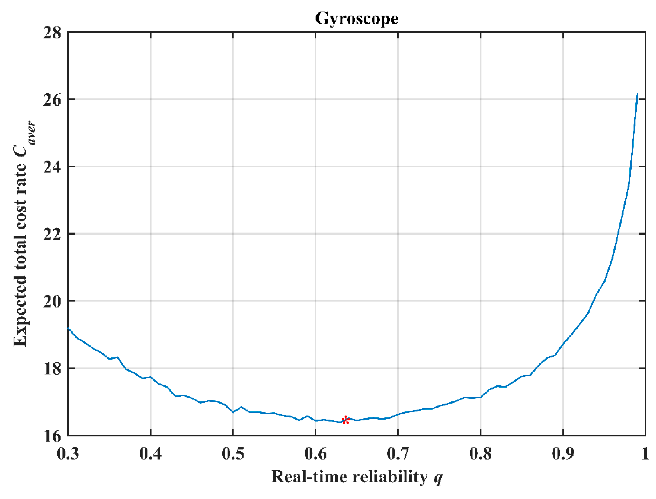
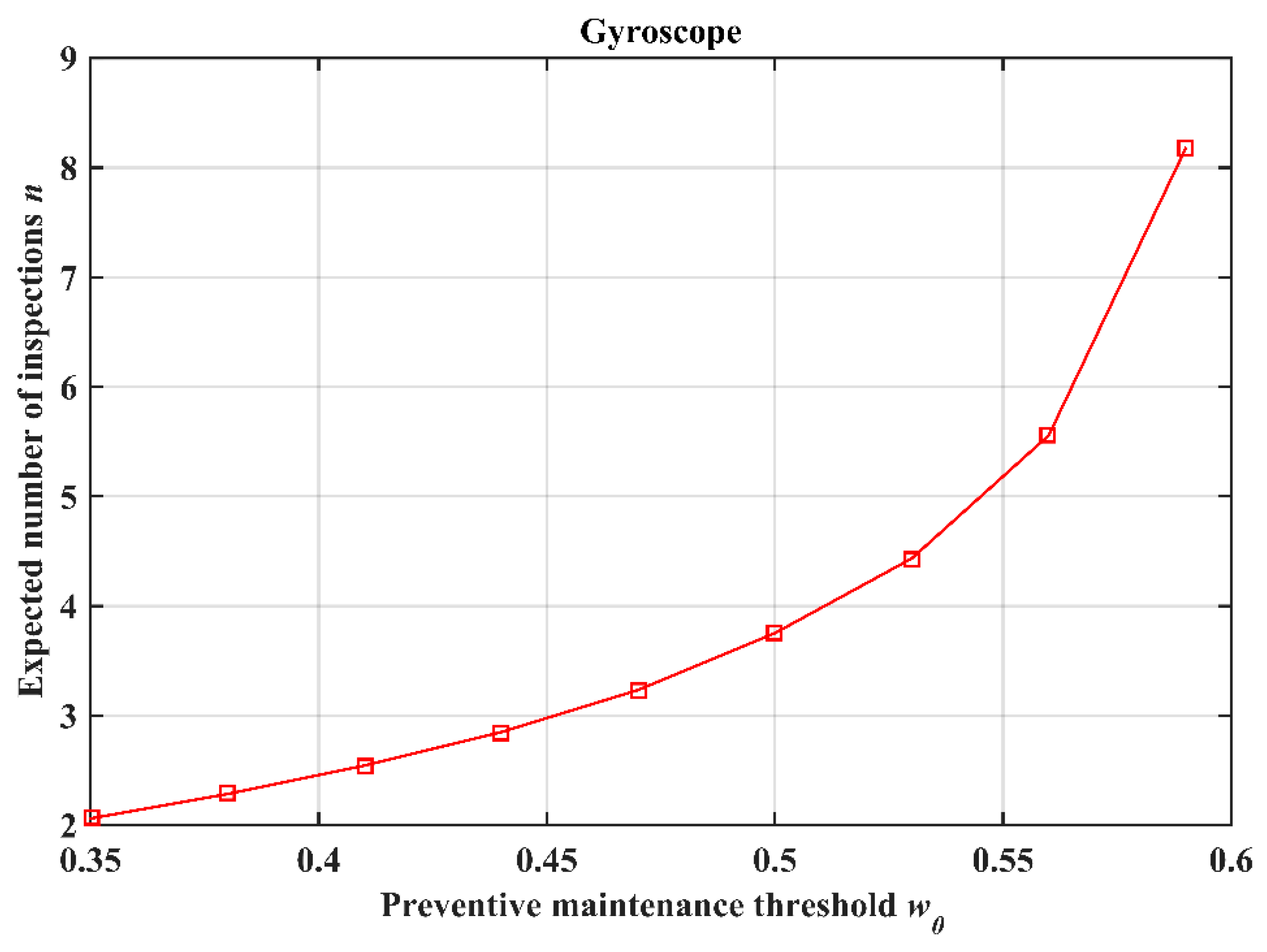
6.1. Maintenance Optimization of the Gyroscope

The inertial navigation system (INS) is a core subsystem of a long-term storage system such as a rocket or missile. Its performance is directly related to the accuracy of navigation and the performance of the control system. As the inertial unit at the heart of the INS, the gyroscope plays a vital role in the entire system. However, during the long-term storage process, due to the influence of environmental stresses and other factors, the performance and reliability of the gyroscope decrease with prolonged storage time, eventually leading to failure of the gyroscope [31]. In addition, gyroscope drift has an effect on the accuracy of the INS. Once the drift exceeds the failure threshold $w$, the gyroscope must be replaced to ensure the INS’s accuracy; otherwise, this drift will cause significant losses. By establishing a reasonable inspection and maintenance strategy, it is possible to effectively prevent the occurrence of such failures. In the following, an example of a gyroscope in an INS is presented to illustrate the method proposed in this paper.

The Wiener process is used to establish a degradation model of the gyroscope drift. The reliability constraint $R^{*}$ for the gyroscope is set to $R^{*}=0.6$, the failure threshold for gyroscope drift is set to $w=0.6\left(°/\mathrm{h}\right)$, and the approximate initial parameters ${\widehat{\theta }}_0={(0.055,0.0004,0.001,0.06)}^T$ are obtained by combining historical data from similar units based on the adaptive estimation method. The cost parameters associated with the inspection and maintenance of the system are shown in

Table 1. Related cost parameters.

${\mathit{C}}_{\mathit{I}}$	${\mathit{C}}_{\mathit{P}}$	${\mathit{C}}_{\mathit{C}}$	${\mathit{C}}_{\mathit{d}}$
20	150	200	50

.

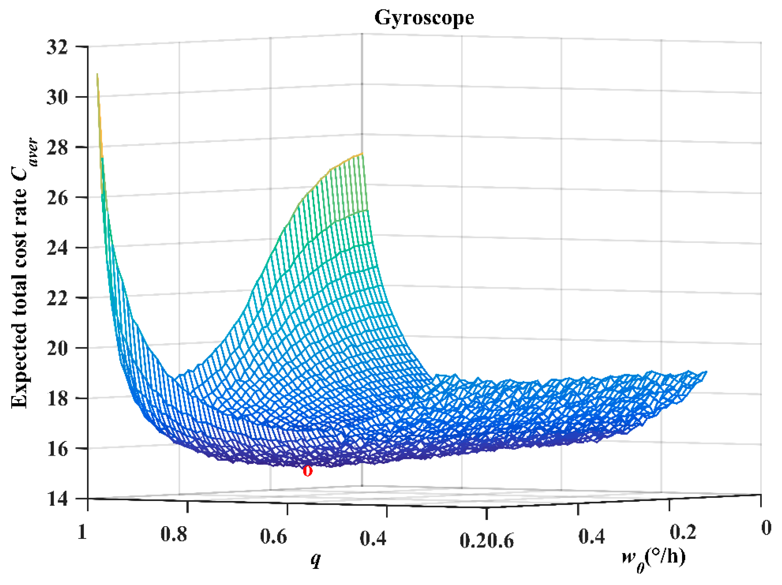
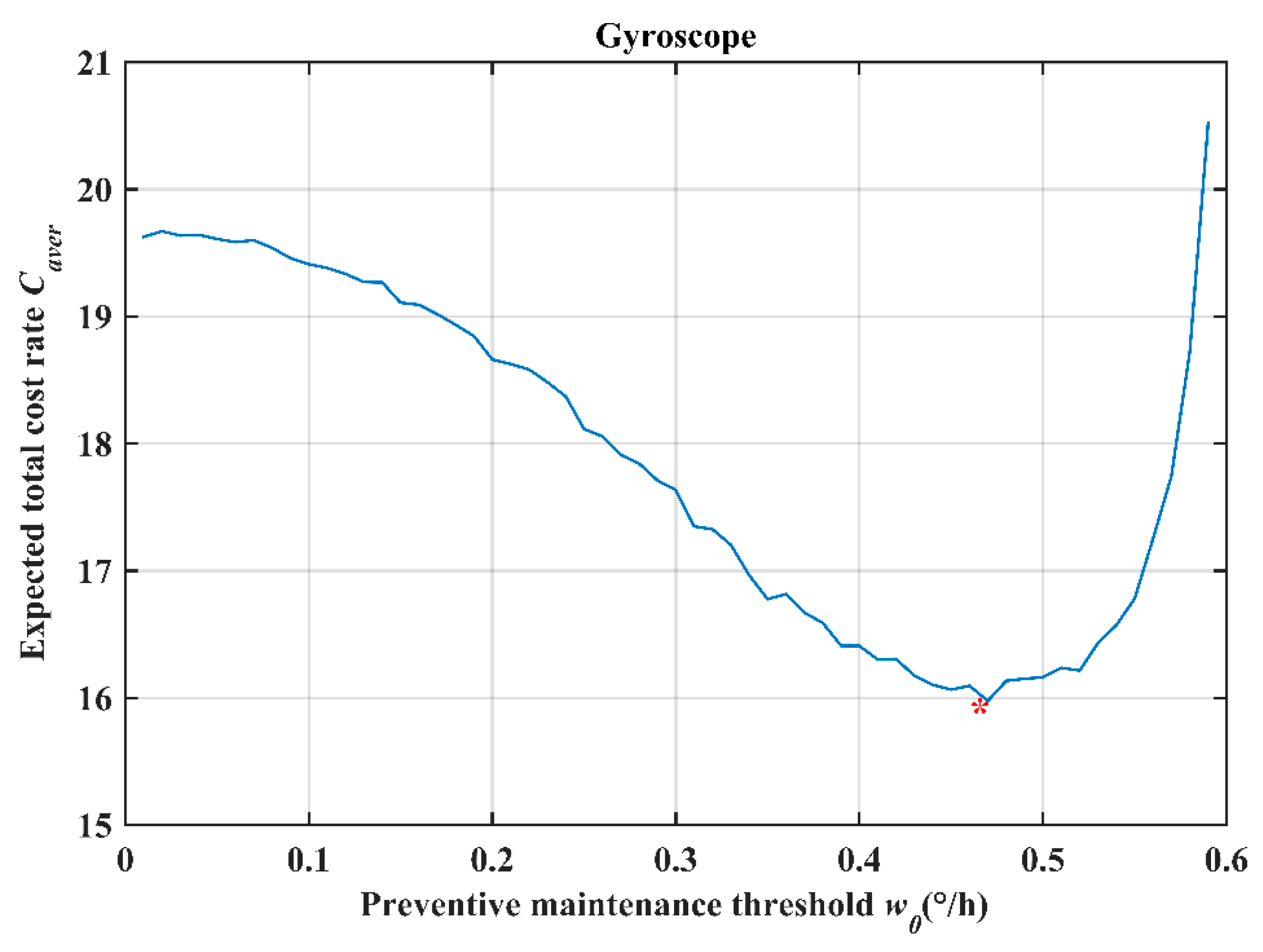
6.1.1. Maintenance Optimization

Through the joint adjustment and optimization analysis, the combination of the optimal values $\left(w_0^{*},q^{*}\right)$ that result in the minimum expected total cost rate can be found. The range of $w_0$ is set to [0.01, 0.59], and the step size is $\Delta w_0=0.01$. The range of $q$ is set to [0.60, 0.99] and the step size is $\Delta q=0.01$. Figure 3 shows the results of the global analysis performed by simulating each combination of parameters $\left(w_0,q\right)$ $n=5000$ times using the Monte Carlo method using the parameter settings given above. The optimal result lies at the position indicated by the “o” symbol in Figure 3.

Figure 3 shows that the optimal values of the decision variables $w_0^{*}$ and $q^{*}$ are $0.48(°/\mathrm{h})$ and $0.68$, respectively, as marked with the “o” symbol in the figure. The corresponding total expected cost rate is $C_{aver}\left(w_0^{*},q^{*}\right)=15.25$.

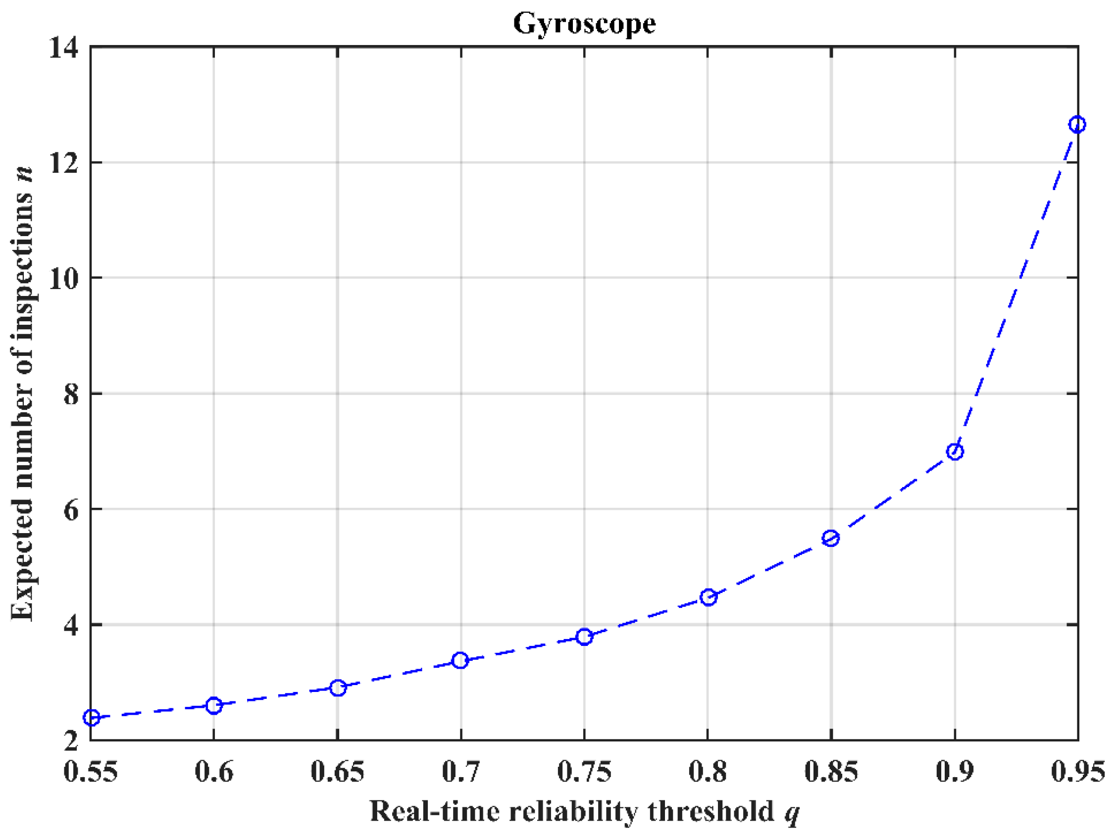
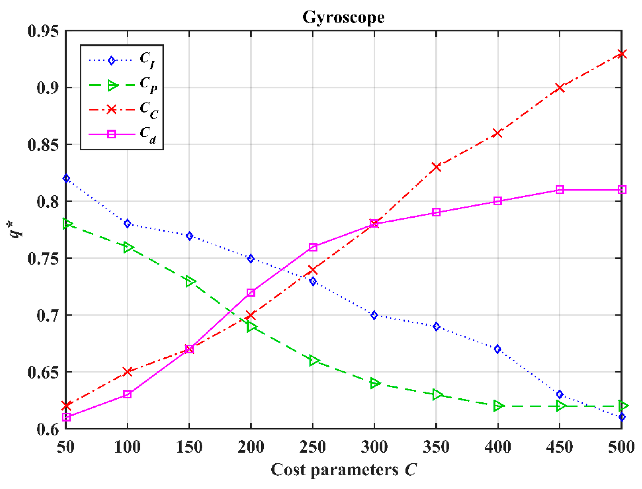
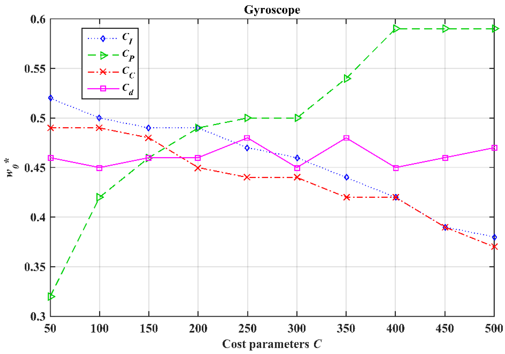
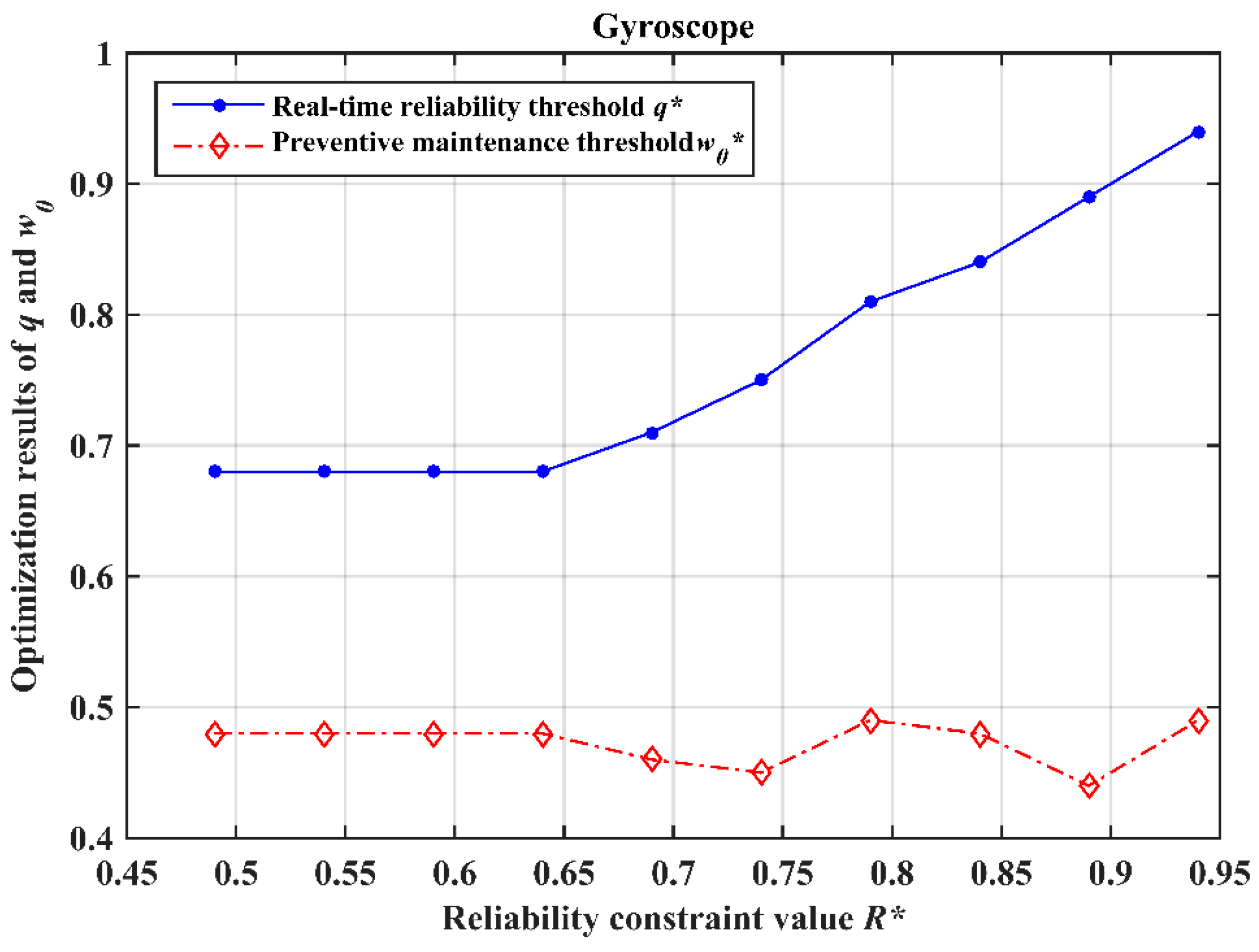
6.1.2. Sensitivity Analysis

The results of maintenance optimization depend on multiple factors. This section will analyze the influences of the real-time reliability threshold $q$, the PM threshold $w_0$, the cost parameters $\left(C_I,C_P,C_C,C_d\right)$, and the reliability constraint value $R^{\ast }$ on the maintenance optimization results.

(1) To analyze the relationship between the expected total cost rate $C_{aver}$, the PM threshold $w_0$, and the real-time reliability threshold $q$, it is necessary to fix the value of one of the parameters $\left(w_0,q\right)$. For example, we assume that the gyroscope is required to be stored with a real-time reliability threshold of $q=0.90$. In this case, the real-time reliability threshold is an input parameter set by the decision-maker rather than a decision variable. The objective of the maintenance decision-maker is then to find the optimal value of the PM threshold $w_0$. Figure 4 shows the variation of the expected total cost rate $C_{aver}$ with the PM threshold $w_0$ when $q=0.90$, where the step size for $w_0$ is $\Delta w_0=0.01$.

As seen from Figure 4, in the case of $q=0.90$, the expected total cost rate first gradually decreases as the PM threshold $w_0$ increases and then gradually rises. The minimum value $Min\left(C_{aver}\right)=15.98$ is obtained at $w_0=0.47\left(°/\mathrm{h}\right)$, as marked with the “*” symbol in the figure. This result is found mainly because the number of instances of PM performed increases when the PM threshold $w_0$ is set to a lower value, meaning that the update cycle H is shorter, which, in turn, increases the expected total cost rate. On the other hand, a higher value of the PM threshold allows long and uninterrupted storage of the system at the cost of an increased risk of failure, which increases the cost of failure loss and the number of inspections, thereby also increasing the expected total cost rate.

Similarly, the relationship between $C_{aver}$ and $q$ can be plotted for the case in which the PM threshold $w_0$ is fixed. Figure 5 depicts the expected total cost rates $C_{aver}$ obtained for different values of the real-time reliability threshold $q$ at $w_0=0.58\left(°/h\right)$, where the step size is $\Delta q=0.01$. The optimal value is $q=0.63$, meaning that the expected total cost rate reaches its minimum when the real-time reliability threshold is set to $q=0.63$. If the real-time reliability threshold $q$ is set to a higher value, more frequent inspections need to be carried out and the number of instances of PM also increases, thus resulting in an increase in the total expected cost rate. On the other hand, a low value of the real-time reliability threshold will permit long and uninterrupted storage of the system, but with an increased probability of failure, which will increase the number of instances of CM and the failure time of the system, thereby increasing the expected total cost rate.

(2) The values of the real-time reliability threshold $q$ and the PM threshold $w_0$ are closely related to the number of inspections. Figure 6 and Figure 7 show the effects of $q$ and $w_0$, respectively, on the expected number of inspections.

As shown in Figure 6 and Figure 7, the expected number of inspections increases as the real-time reliability threshold $q$ and the PM threshold $w_0$ increase. This behavior occurs because the larger the real-time reliability threshold $q$ or the PM threshold $w_0$ is, the longer the system update cycle will be, meaning that more inspections will be required.

(3) The maintenance cost parameters are directly related to the maintenance optimization results. Figure 8 and Figure 9 show the influence of the cost parameters on the optimal values $q^{*}$ and $w_0^{*}$, respectively. The variation range of each cost parameter in Figure 8 and Figure 9 is [50, 500].

As shown in Figure 8, $q^{*}$ gradually decreases as $C_I$ increases. This is because, according to Figure 6, the number of inspections can be reduced by lowering $q^{*}$, thereby reducing the influence of an increase in $C_I$ on the expected total cost rate $C_{aver}$. Moreover, reducing $q^{*}$ will increase the probability of system failure, thus making the maintenance activities more likely to be of the CM type; therefore, $q^{*}$ decreases as $C_P$ increases, thus reducing the influence of an increase in $C_P$ on $C_{aver}$. Conversely, the probability of system failure can be reduced by increasing $q^{*}$, thus making the maintenance activities more likely to be of the PM type and consequently reducing the influence of an increase in $C_C$ on $C_{aver}$. In addition, increasing $q^{*}$ also reduces the failure time of the system by reducing the probability of system failure, thereby reducing the influence of an increase in $C_d$ on $C_{aver}$. Therefore, $q^{*}$ increases as $C_d$ increases.

Figure 9 shows the influence of changes in the cost parameters on $w_0^{*}$. As $C_I$ increases, $w_0^{*}$ exhibits a downward trend. This is because the number of inspections can be reduced by lowering $w_0^{*}$, thereby achieving a reduction in the influence on the expected total cost rate $C_{aver}$. Similarly, the likelihood of PM can be increased by lowering $w_0^{*}$, thus reducing the influence on $C_{aver}$ of an increase in $C_C$. By contrast, $w_0^{*}$ shows an upward trend with increasing $C_P$ because increasing $w_0^{*}$ can extend the uninterrupted storage time of the system and make the maintenance activities more likely to be of the CM type while seeking the optimal expected total cost rate $C_{aver}$. Figure 9 also shows that an increase in $C_d$ has no obvious influence on $w_0^{*}$.

(4) It is currently assumed that a long-term storage system is required to be stored with a given reliability constraint value $R^{*}$; thus, we should find an optimal maintenance policy that can satisfy this demand. According to the proposed maintenance policy, we simply take the real-time reliability threshold to satisfy $R^{*}\le q<1$. This means that the optimal policy can be found by varying the values of the PM threshold $w_0$ and the real-time reliability threshold $q$ accordingly. Figure 10 shows the influence of the reliability constraint value $R^{*}$ on the optimal values of the real-time reliability threshold $q$ and the PM threshold $w_0$, respectively.

As shown in Figure 10, as the reliability constraint value $R^{*}$ increases from 0.49 to 0.68, the optimal values $q^{*}$ and $w_0^{*}$ remain unchanged at 0.68 and $0.48(°/\mathrm{h})$, respectively. This is because when $R^{*}$ is small $\left(R^{*}\le 0.68\right)$, as seen from Figure 3, the global optimization results for $q$ and $w_0$ are $q^{*}=0.68$ and $w_0^{*}=0.48\left(°/\mathrm{h}\right)$, respectively, and remain unchanged over the interval [0.49,0.68]. However, when $R^{*}>0.68$, $q^{*}$ shows an upward trend as $R^{\ast }$ continues to increase, mainly because of the need to satisfy the reliability constraint for the system; consequently, the optimization result for $q$ can simply be approximated as $q=R^{*}$. By contrast, it can be seen from Figure 10 that as $R^{*}$ continues to increase, $w_0^{*}$ fluctuates around $0.48(°/\mathrm{h})$, indicating that $R^{*}$ has little effect on the optimization result for $w_0$. Indeed, this fluctuation of $w_0^{*}$ around $0.48(°/\mathrm{h})$ proves the robustness and applicability of the proposed optimization model.

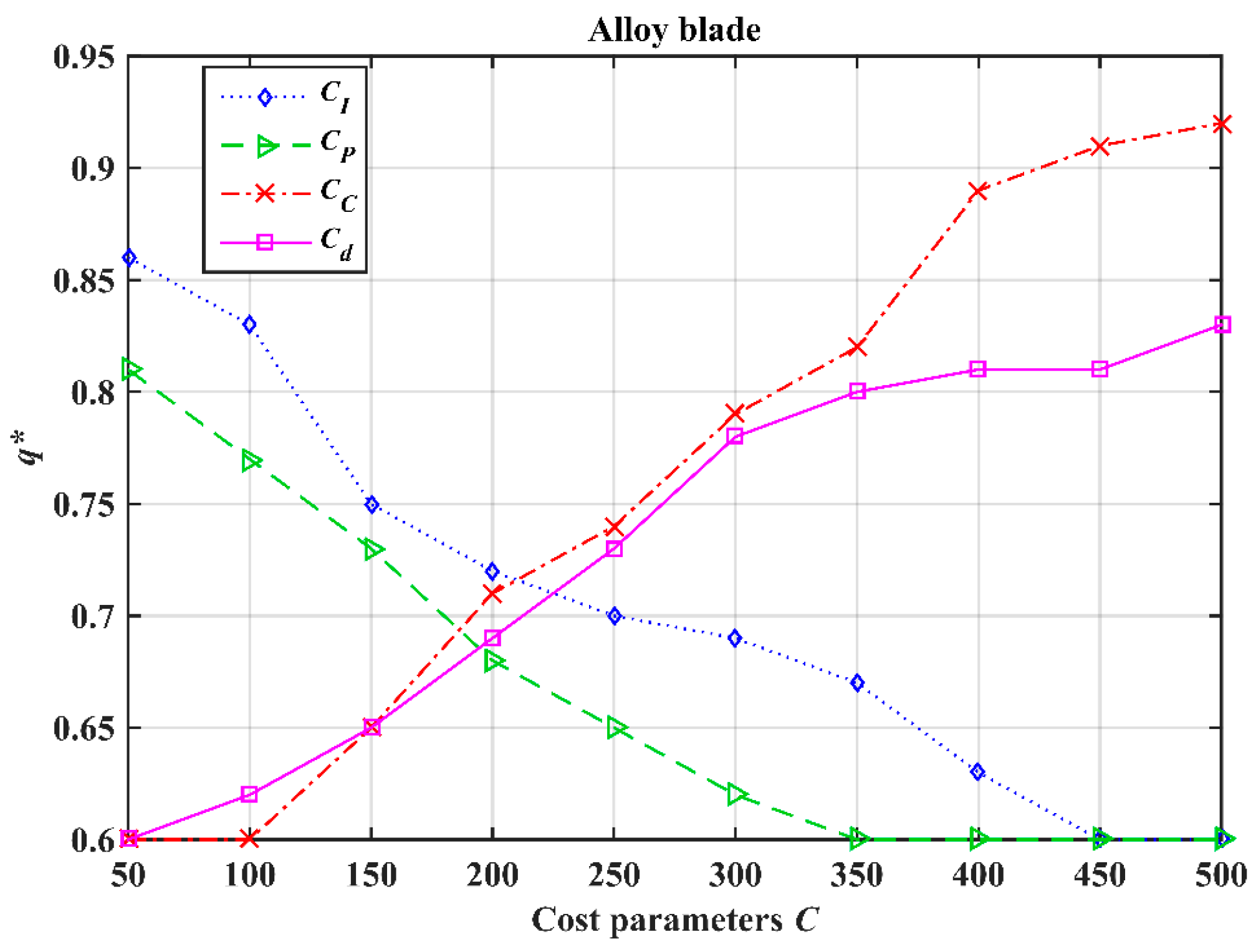
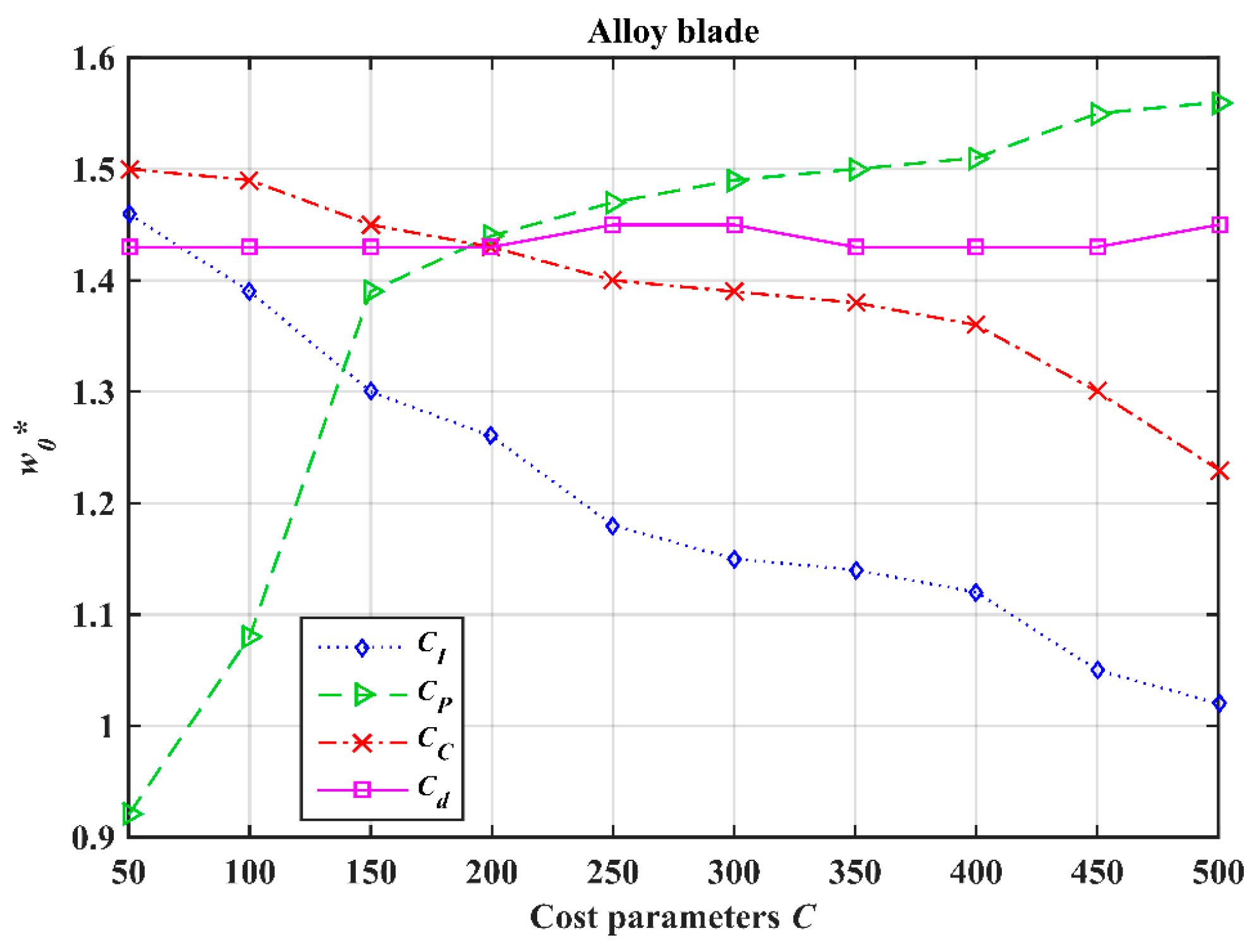
6.2. Maintenance Optimization of the Alloy Blade

Alloy blades are the key components of rocket engines, and their reliability directly determines the flight performance of long-storage systems. During long storage, the crack length of the blade will gradually increase due to various environmental stresses. Therefore, the quality of this alloy material is generally evaluated by the length of the crack. All alloy blade cracks have an initial length of 0.9 inches (1 inch = 2.54 cm) [32] and are considered to be invalid when the crack length reaches 1.6 inches (1 inch = 2.54 cm), i.e., the failure threshold is $w=1.6$ inches (1 inch =2.54 cm), the time unit of crack growth in alloy blade is per million cycles, and the approximate initial parameters ${\widehat{\theta }}_0={(6.5,0.5,0.5,0.1)}^T$ are obtained by combining historical data from similar units based on the adaptive estimation method. The relevant cost parameters are $C_I=50$, $C_P=200$, $C_C=250$, and $C_d=100$ respectively.

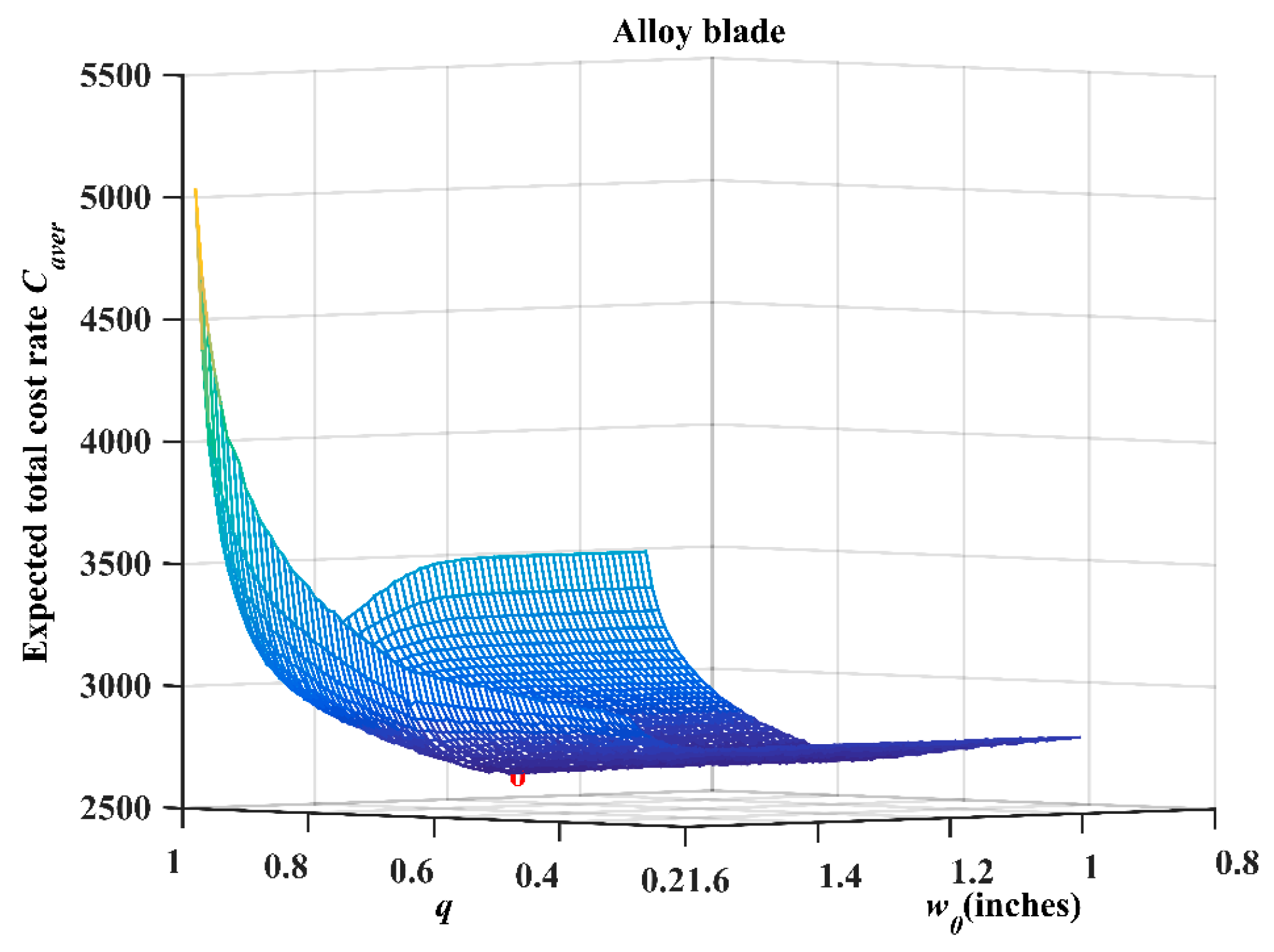
6.2.1. Optimization Results of Alloy Blades

Similar to the simulation optimization method of the gyroscope, the range of $w_0$ is set to [0.91, 1.59], and the step size is $\Delta w_0=0.01$. The range of $q$ is set to [0.60, 0.99], and the step size is $\Delta q=0.01$. Figure 11 shows the results of global analysis of the alloy blades, and the optimal result lies at the position indicated by the “o” symbol.

It can be seen from Figure 11 that the optimization results of $w_0^{*}$ and $q^{*}$ are 1.43 inches (1 inch = 2.54 cm) and 0.66, respectively, and the corresponding total expected cost rate is $C_{aver}\left(w_0^{*},q^{*}\right)=2659.5$.

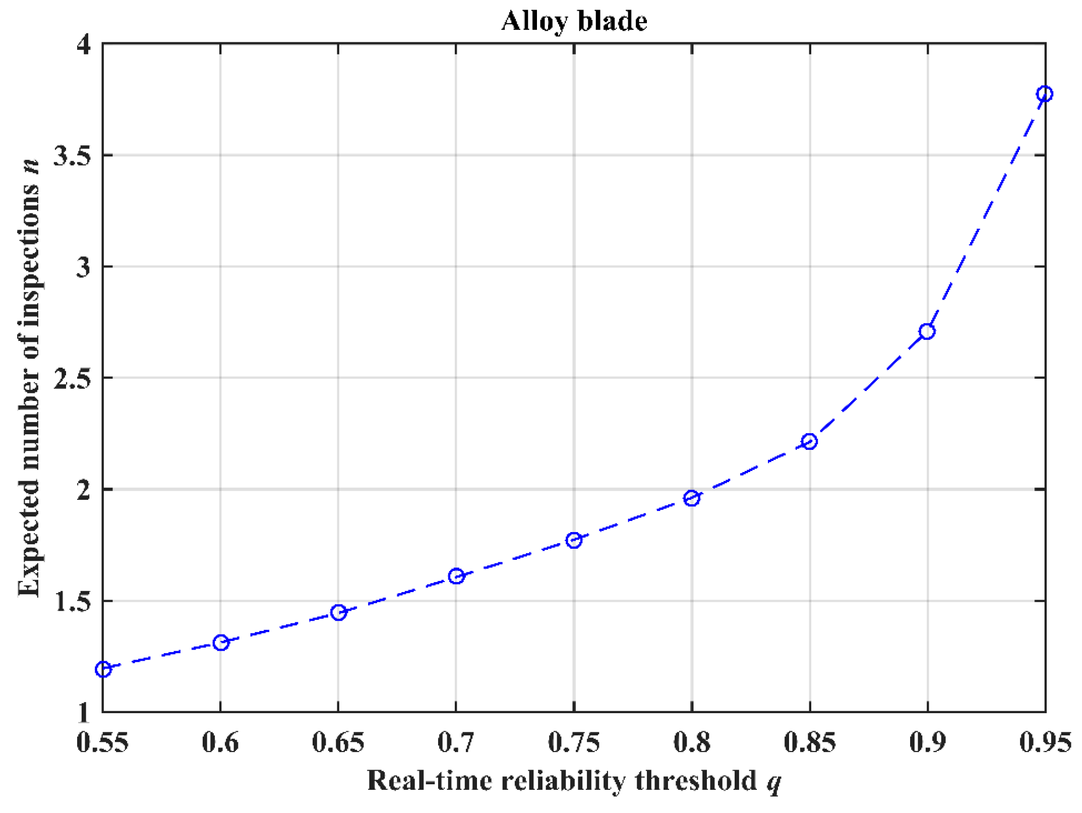
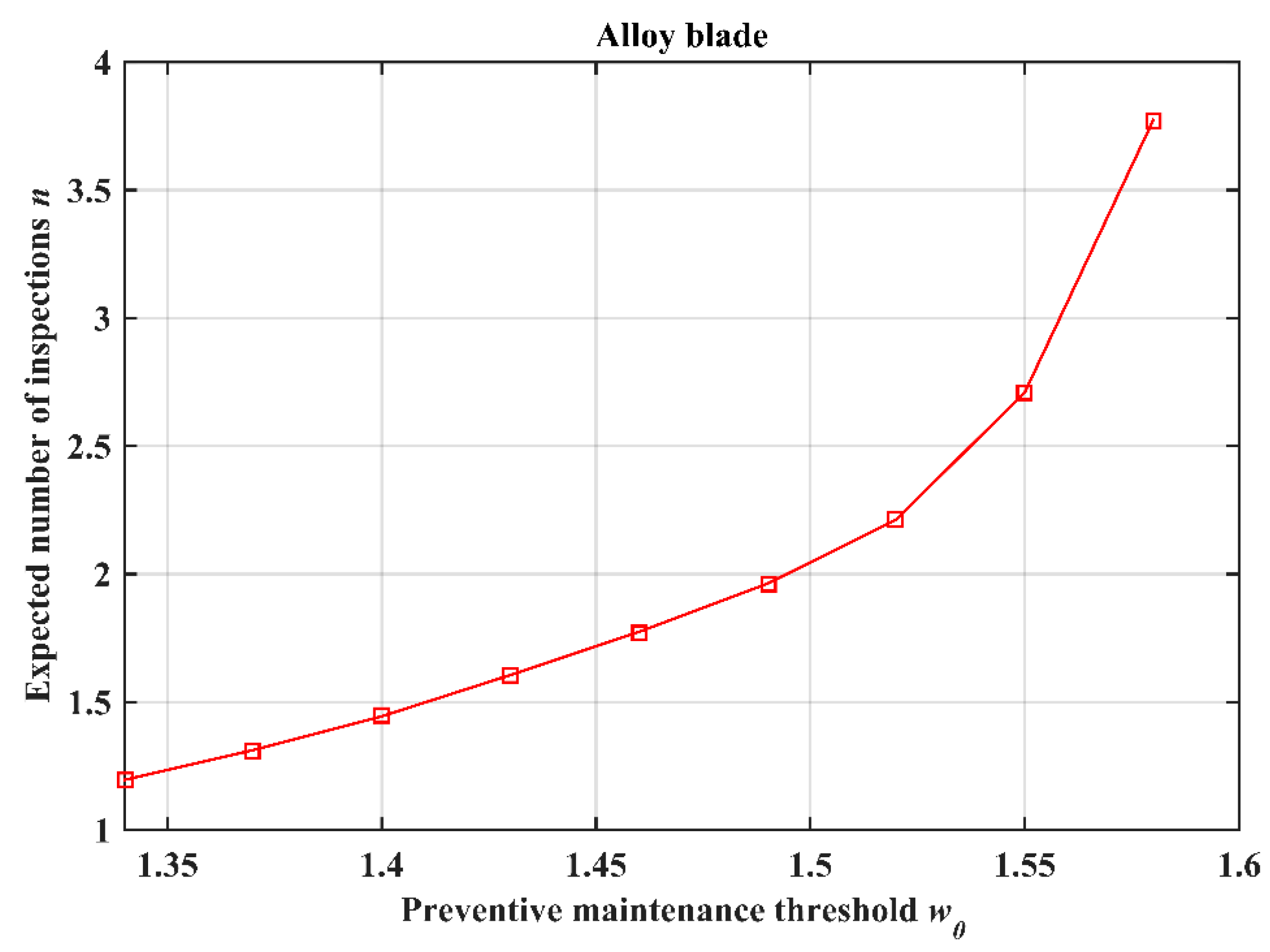
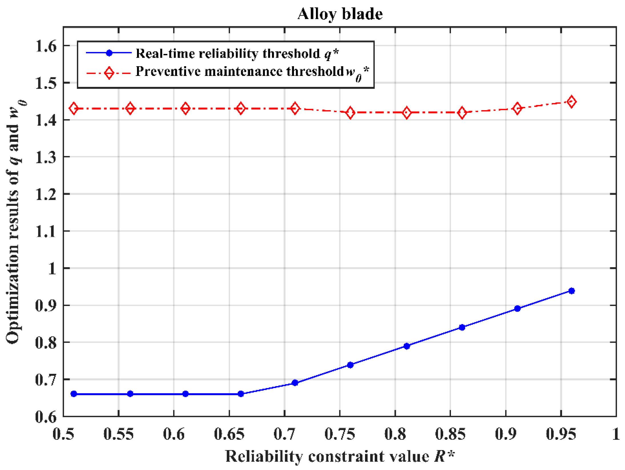
6.2.2. Sensitivity Analysis

Similar to the method used to analyze gyroscopes, sensitivity analysis of relevant parameters of alloy blades is carried out in this section.

(1) Figure 12 and Figure 13 show the effects of $q$ and $w_0$, respectively, on the expected number of inspections. As shown in these two Figures, the expected number of inspections increases as the real-time reliability threshold $q$ and the PM threshold $w_0$ increase, as in the case of the gyroscope unit.

(2) Figure 14 and Figure 15 show the influence of the cost parameters on the optimal values $q^{*}$ and $w_0^{*}$, respectively, and the variation range of each cost parameter is also set to be [50, 500].

As can be seen from Figure 14 and Figure 15, their curve changes show similar trends as Figure 8 and Figure 9, respectively. Through specific analysis, the relevant reasons for this situation are similar to those in the gyroscope case study and are limited to the length of the paper, they will not be described in detail here. For details, please refer to the analysis part of the gyroscope case study.

(3) Figure 16 shows the influence of the reliability constraint value $R^{*}$ on the optimal values of the real-time reliability threshold $q$ and the PM threshold $w_0$, respectively.

As shown in Figure 16, as the reliability constraint value $R^{*}$ increases from 0.5 to 0.66, the optimal values $q^{*}$ and $w_0^{*}$ remain unchanged at 0.66 and 1.43 inches (1 inch =2.54 cm), respectively. Then, when $R^{\ast }>0.66$, $q^{\ast }$ shows an upward trend as $R^{\ast }$ continues to increase; this is also mainly because of the need to satisfy the reliability constraint for the system, such as the analysis of the gyroscope case. Besides, it can be seen from Figure 16 that as $R^{*}$ continues to increase, $w_0^{*}$ fluctuates around 1.43 inches (1 inch = 2.54 cm), also indicating that $R^{*}$ has little effect on the optimization result for $w_0$.

Through the maintenance optimization modeling of the gyroscope and the alloy blade, the maintenance optimization model proposed in this paper is analyzed from two levels: the device level and the component level, respectively, which verifies the effectiveness of the model, thus can provide support for the maintenance decision of long-term storage system.

7. Conclusions

To ensure the safety and reliability of long-term storage systems and improve the efficiency of inspection and maintenance, a maintenance optimization model with sequential inspection is proposed in this paper based on real-time reliability evaluation. It is known that during the actual long-term storage of a system, the mechanisms of performance degradation are complex, and the degradation process itself shows a certain level of randomness. By means of real-time reliability assessment and sequential inspection, the relevant parameters of the degradation model can be adaptively updated, allowing the inspection interval for the system to be adjusted in real-time in accordance with the observed system state, thereby improving the adaptability of the inspection strategy to the dynamic system degradation process. This method can ensure the reliability of a long-term storage system while avoiding the problems of overinspection and underinspection that may be encountered in the traditional case of equal-length inspection cycles. In addition, an analytical expression for the expected total cost rate of inspection and maintenance is presented based on update process theory, and the use of Monte Carlo simulations is proposed to obtain the optimal values of the real-time reliability threshold and the preventive maintenance threshold for the critical unit of interest, thereby providing theoretical support for the scientific development of inspection and maintenance strategies. Finally, through a sensitivity analysis of the cost parameters, the real-time reliability threshold, the preventive maintenance threshold and the system reliability constraint value, the effectiveness of the proposed maintenance optimization model is proven.

The research reported in this paper was carried out under the assumption of perfect product maintenance. In order to reduce the complexity of the model and better derive the analytical expression of the optimization model, this paper assumed that the performance state of the unit would be restored to the same level as when the unit was new after preventive maintenance (PM). In some cases, however, the performance of a product as a whole is affected by certain nonreplaceable parts and various environmental factors affecting the system, thus the “new” state will contain a mixture of systems of different ages, depending on how recently each system returned to this state; like-new performance cannot be recovered after maintenance. Therefore, considering a similar maintenance method for a product in the case of imperfect maintenance is a topic for further study.

References

1. Alaswad, S.; Xiang, Y.S. A review on condition-based maintenance optimization models for stochastically deteriorating system. Reliab. Eng. Syst. Saf. 2017, 157, 54–63. [Google Scholar] [CrossRef]
2. Ballesteros, A.; Sanda, R.; Maqua, M.; Stephan, J.L. Maintenance related events in nuclear power stations. Eksplo. i. Nieza. -Maint. Relia. 2017, 19, 26–30. [Google Scholar] [CrossRef]
3. Marseguerra, M.; Zio, E.; Podofillini, L. Condition-based maintenance optimization by means of genetic algorithms and Monte Carlo simulation. Reliab. Eng. Syst. Saf. 2002, 77, 151–165. [Google Scholar] [CrossRef]
4. Barata, J.; Soares, C.G.; Marseguerra, M.; Zio, E. Simulation modelling of repairable multi-component deteriorating systems for ‘on condition’ maintenance optimization. Reliab. Eng. Syst. Saf. 2002, 76, 255–264. [Google Scholar] [CrossRef]
5. Zhou, X.J.; Xi, L.F.; Lee, J. Reliability-centered predictive maintenance scheduling for a continuously monitored system subject to degradation. Reliab. Eng. Syst. Saf. 2007, 92, 530–534. [Google Scholar] [CrossRef]
6. Tian, Z.G.; Jin, T.D.; Wu, B.R.; Ding, F.F. Condition based maintenance optimization for wind power generation systems under continuous monitoring. Renew. Energy 2011, 36, 1502–1509. [Google Scholar] [CrossRef]
7. Tang, D.; Sheng, W.; Yu, J. Dynamic condition-based maintenance policy for degrading systems described by a random-coefficient autoregressive model: A comparative study. Eksplo. Nieza. Maint. Reliab. 2018, 20, 590–601. [Google Scholar] [CrossRef]
8. Liao, H.; Elsayed, E.A.; Chan, L.Y. Maintenance of continuously monitored degrading systems. Eur. J. Oper. Res. 2006, 175, 821–835. [Google Scholar] [CrossRef]
9. Liu, X.; Li, J.R.; Al-Khalifa, K.N.; Hamouda, A.S.; Coit, D.W.; Elsayed, E.A. Condition-based maintenance for continuously monitored degrading systems with multiple failure modes. IIE Trans. 2013, 45, 422–435. [Google Scholar] [CrossRef]
10. Besnard, F.; Bertling, L. An approach for condition-based maintenance optimization applied to wind turbine blades. IEEE Trans. Sustain. Energy 2010, 1, 77–83. [Google Scholar] [CrossRef]
11. Shi, L.Y.; Zhang, R.; Song, W.Y. Method of Determining Check Period during Storage of Missile Weapon System. Tacti Missile Technol. 2004, 3, 22–25. [Google Scholar] [CrossRef]
12. Fan, Z.F.; Xu, J.Q.; Cui, P.; Guo, G.H. Optimal Study on Detection Period of a New-style Rocket Projectile. J. Proj. Rocket Missiles Guid. 2016, 36, 163–165. [Google Scholar] [CrossRef]
13. Zhang, J.C.; Liu, C. Analysis of the influence of Periodic Check on Reliability of Missile Weapon System. Tacti Missile Technol. 2008, 3, 44–48. [Google Scholar] [CrossRef]
14. Hajipour, Y.; Taghipour, S. Non-Periodic Inspection Optimization of Multi-Component and k-out-of-m Systems. Reliab. Eng. Syst. Saf. 2016, 156, 228–243. [Google Scholar] [CrossRef]
15. Yan, H.C.; Zhou, J.H.; Pang, C.K. Machinery Degradation Inspection and Maintenance Using a Cost-Optimal Non-Fixed Periodic Strategy. IEEE Trans. Instrum. Meas. 2016, 65, 2067–2077. [Google Scholar] [CrossRef]
16. Jiang, R. Optimization of alarm threshold and sequential inspection scheme. Reliab. Eng. Syst. Saf. 2010, 95, 208–215. [Google Scholar] [CrossRef]
17. Zhao, X.; Al-Khalifa, K.N.; Nakagawa, T. Approximate Methods for Optimal Replacement, Maintenance, and Inspection Policies. Reliab. Eng. Syst. Saf. 2015, 144, 68–73. [Google Scholar] [CrossRef]
18. Zhu, Z.C.; Xiang, Y.S.; Alaswad, S.; Cassady, C.R. A sequential inspection and replacement policy for degradation-based systems. In Proceedings of the 2017 Annual Reliability and Maintainability Symposium (RAMS), Orlando, FL, USA, 23–26 January 2017; IEEE: Piscataway, NJ, USA, 2017. [Google Scholar] [CrossRef]
19. Yan, W.A.; Song, B.W.; Duan, G.L.; Shi, Y.M. Real-Time Reliability Evaluation of Two-Phase Wiener Degradation Process. Commun. Stat.-Theory Methods 2017, 46, 176–188. [Google Scholar] [CrossRef]
20. Wang, X.; Jiang, P.; Guo, B.; Cheng, Z. Real-time reliability evaluation with a general wiener process-based degradation model. Qual. Reliab. Eng. Int. 2014, 30, 205–220. [Google Scholar] [CrossRef]
21. Zhang, Y.; Li, S.W. A Study on the Real-Time Reliability of on-Board Equipment of Train Control System. IOP Conf. Ser. Mater. Sci. Eng. 2018, 351, 1–14. [Google Scholar] [CrossRef]
22. Guo, C.M.; Guo, B.; Wang, W.B.; Peng, R. Maintenance optimization under non-periodic imperfect inspections. J. Natl. Univ. Def. Technol. 2013, 35, 176–181. [Google Scholar] [CrossRef]
23. Ito, K.; Nakagawa, T. Optimal Inspection Policies for a Storage System with Degradation at Periodic Tests. Math. Comput. Model. 2000, 31, 191–195. [Google Scholar] [CrossRef]
24. Hoseinie, S.H.; Ghodrati, B.; Galar, D.; Juuso, E. Optimal Preventive Maintenance Planning for Water Spray System of Drum Shearer. IFAC-Pap. 2015, 48, 166–170. [Google Scholar] [CrossRef]
25. Tan, C.M.; Narula, U.; Pandey, S. Optimal maintenance strategy on medical instruments used for haemodialysis process. Eksploat. Niezawodn. Maint. Reliab. 2019, 21, 318–328. [Google Scholar] [CrossRef]
26. Khatab, A. Maintenance optimization in failure-prone systems under imperfect preventive maintenance. J. Intell. Manuf. 2018, 29, 707–717. [Google Scholar] [CrossRef]
27. Wang, X.L.; Guo, B.; Cheng, Z.J. Real-time reliability evaluation for product with nonlinear drift-based Wiener process. J. Cent. South Univ. 2013, 44, 3203–3209. [Google Scholar]
28. Si, X.S.; Wang, W.; Hu, C.H.; Chen, M.Y.; Zhou, D.H. A Wiener-process-based degradation model with a recursive filter algorithm for remaining useful life estimation. Mech. Syst. Signal. Process. 2013, 35, 219–237. [Google Scholar] [CrossRef]
29. Bai, S.Y.; Cheng, Z.J.; Guo, B.; Yang, Y. Sequential inspection model for aviation product based on real real-time reliability. J. Mech. Eng. 2019, 55, 177–185. [Google Scholar] [CrossRef]
30. Ross, S.M. Introduction to Probability Models, 9th ed.; Academic Press: Orlando, FL, USA, 2008; pp. 71–80. [Google Scholar] [CrossRef]
31. Si, X.S.; Chen, M.; Wang, W.; Hu, C.H.; Zhou, D.H. Specifying measurement errors for required lifetime estimation performance. Eur. J. Oper. Res. 2013, 231, 631–644. [Google Scholar] [CrossRef]
32. Meeker, W.Q.; Escobar, L.A. Statistical Methods for Reliability Data; Wiley: New York, NY, USA, 1998. [Google Scholar] [CrossRef]
Figure 1. Flow chart of the process of sequential inspection and maintenance optimization.
Processes 07 00481 g001
Figure 2. Schematic diagram of the unit degradation and maintenance process.
Processes 07 00481 g002
Figure 3. The relationship between the expected total cost rate C a v e r , the PM threshold w 0 , and the real-time reliability threshold q .
Processes 07 00481 g003
Figure 4. Total expected cost rate C a v e r versus the PM threshold w 0 when q = 0.90 .
Processes 07 00481 g004
Figure 5. Total expected cost rate C a v e r versus the real-time reliability threshold q when w 0 = 0.58 ( ° / h ) .
Processes 07 00481 g005
Figure 6. Total expected number of inspections versus the real-time reliability threshold q at w 0 = 0.58 ( ° / h ) .
Processes 07 00481 g006
Figure 7. Total expected number of inspections versus the PM threshold w 0 at q = 0.90 .
Processes 07 00481 g007
Figure 8. Influence of the cost parameters on the optimal value q .
Processes 07 00481 g008
Figure 9. Influence of the cost parameters on the optimal value w 0 .
Processes 07 00481 g009
Figure 10. Sensitivity analysis of the effects of the reliability constraint value R * on the optimal values q * and w 0 * .
Processes 07 00481 g010
Figure 11. The relationship between the expected total cost rate C a v e r , the PM threshold w 0 and the real-time reliability threshold q .
Processes 07 00481 g011
Figure 12. Total expected number of inspections versus the real-time reliability threshold q at w 0 = 1.58 inches (1 inch = 2.54 cm).
Processes 07 00481 g012
Figure 13. Total expected number of inspections versus the PM threshold w 0 at q = 0.95 .
Processes 07 00481 g013
Figure 14. Influence of the cost parameters on the optimal value q * .
Processes 07 00481 g014
Figure 15. Influence of the cost parameters on the optimal value w 0 * .
Processes 07 00481 g015
Figure 16. Sensitivity analysis of the effects of the reliability constraint value R * on the optimal values q * and w 0 * .
Processes 07 00481 g016