Article

A Method and Device for Detecting the Number of Magnetic Nanoparticles Based on Weak Magnetic Signal

1
School of Electrical Engineering, Henan University of Technology, Zhengzhou 450007, China
2
School of Sciences, Henan University of Technology, Zhengzhou 450007, China
*
Author to whom correspondence should be addressed.
Processes 2019, 7(8), 480; https://doi.org/10.3390/pr7080480
Submission received: 22 April 2019 / Revised: 17 July 2019 / Accepted: 19 July 2019 / Published: 25 July 2019
(This article belongs to the Section Advanced Digital and Other Processes)

Abstract

:
In recent years, magnetic nanoparticles (MNPs) have been widely used as a new material in biomedicine and other fields due to their broad versatility, and the quantitative detection method of MNPs is significantly important due to its advantages in immunoassay and single-molecule detection. In this study, a method and device for detecting the number of MNPs based on weak magnetic signal were proposed and machine learning methods were applied to the design of MNPs number detection method and optimization of detection device. Genetic Algorithm was used to optimize the MNPs detection platform and Simulated Annealing Neural Network was used to explore the relationship between different positions of magnetic signals and the number of MNPs so as to obtain the optimal measurement position of MNPs. Finally, Radial Basis Function Neural Network, Simulated Annealing Neural Network, and partial least squares multivariate regression analysis were used to establish the MNPs number detection model, respectively. Experimental results show that Simulated Annealing Neural Network model is the best among the three models with detection accuracy of 98.22%, mean absolute error of 0.8545, and root mean square error of 1.5134. The results also indicate that the method and device for detecting the number of MNPs provide a basis for further research on MNPs for the capture and content analysis of specific analyte and to obtain other related information, which has significant potential in various applications.

1. Introduction

With the rapid development of nanotechnology, magnetic nanoparticles (MNPs), as a new material with high practical value and broad versatility, have been widely used in biomedicine, chemical catalysis, immunoassay, and magnetic detection due to their unique superparamagnetism and magnetic manipulation [1]. When the surfaces of MNPs are modified with different active groups, they can be applied to cell sorting [2], rapid detection of microorganisms, purification of proteins [3], separation and purification of nucleic acids [4], and specific capture of analytes. By detecting the MNPs quantitatively, the specific content information of the analyte can be obtained. At the same time, MNPs, as magnetic material, have magnetic properties. Techniques such as magneto–electricity, magneto–optical, magneto–thermal, and other methods can be used to detect the weak magnetic signal of MNPs. Compared to traditional detection methods, MNP detection based on weak magnetic signal has a series of advantages, such as short measurement time, strong penetrability, simple sample processing, and less external interference.
In recent years, with the rapid development of micro-electromechanical systems (MEMS) technology [5], microfluidic technology, also known as Lab on a Chip [6], has been widely used in the field of magnetic detection, realizing the miniaturization and integration of magnetic detection devices. Combined with the detection of weak magnetic signal, microfluidic technology can realize real-time detection of the content of a variety of analytes in case of very small sample and reagent consumption [7]. The MNP device, with micro–nano level thickness, investigated in this study was manufactured by microfluidic technology.
Currently, the methods of quantitative detection based on magnetic properties of MNPs or the influence on the surrounding magnetic field are mainly divided into three categories, namely coil-based induction technology, magnetic sensor-based detection technology, and indirect measurement method for analyzing the influence of MNPs on the surrounding environment. Simmonds et al. [8] introduced ferromagnetic fluid into the coil of a measuring device, changed the inductance of the coil, and considered that the voltage change measured by Maxwell bridge was proportional to the concentration of magnetic fluid, so as to realize the detection of the number of MNPs. Superconducting quantum interference device (SQUID), as a type of highly sensitive magnetic sensor, was first introduced into the field of MNP detection by Kotitz et al. [9]. The number of MNPs can be detected by measuring their relaxation time or the change of the magnetization rate of alternating current [10]. Nuclear magnetic resonance (NMR) technology, as a type of highly sensitive magnetic field detection method, based on the local magnetic field of MNPs, influences the nuclear spin coherent motion of the neighboring water protons [11]. It can thus realize indirect number measurement of MNPs, also known as the diagnostic magnetic resonance (DMR). Issadore et al. [12] developed a miniature DMR system called DMR-3. However, currently available methods for the detection of number of MNPs encounter some problems such as high cost, complex methods, and imprecise equipment parameter setting. The detection method for the number of MNPs based on microfluidic technology has become an important research direction to further shorten the detection time, lower the cost, and reduce the amount of samples used. How to accurately set different parameters of the detection platform and select a reasonable detection location have also become limitations to be resolved in the process of improving the detection accuracy of the number of MNPs.
Machine learning, which mainly studies the simulation and implementation of human learning behavior [13,14], is an important branch of artificial intelligence, including Neural Network, Support Vector Machine, and other algorithms, and is increasingly widely used in MNPs detection. Yan et al. [15] used Support Vector Machine to classify weak positive and negative samples in the quantitative detection of MNPs on the immunochromatographic test strips, so as to improve the accuracy of quantitative detection. Khosravi et al. [16] used various machine learning methods to predict the heat transfer coefficient (HTC) of Fe3O4 nanoparticles in water.
This study proposed a method and device for detecting the number of MNPs based on weak magnetic signal for microfluidic control technology in which MNPs were used as carriers to specifically capture analytes. The study mainly included the optimization method of MNP detection device and the selection method of the optimal detection position of MNPs and finally established the quantitative detection model to realize the accurate detection of the number of MNPs. In this study, machine learning method and finite element analysis method were combined to optimize the MNP detection platform and design the quantitative detection method. The MNP detection platform was optimized by using Genetic Algorithm to minimize the influence of parameter setting of the detection platform on the accuracy of the number measurement of MNPs, so as to make the magnetic field generated by the detection platform meet the requirements of MNPs detection. According to the results of the optimization of Genetic Algorithm, by changing the number of MNPs, combined with the conditions of magnetic reunion, simulation experiments with uniform magnetic field were carried out to establish a sample set of machine learning. The relationship between the weak magnetic signal at different positions and the number of MNPs was explored through the Simulated Annealing Neural Network algorithm, and the optimal detection position of MNPs was finally obtained. At the optimal detection position, based on Radial Basis Function (RBF) Neural Network [17], Simulated Annealing Neural Network [18], and partial least squares (PLS) multivariate regression analysis [19], the relationship between the weak magnetic signal and the number of MNPs was established, and the detection model of the number of MNPs was constructed, providing a basis for the follow-up study on the content of specific capture analytes of MNPs.

2. Design and Optimization of Detection Platform

2.1. Design of Detection Platform

Combined with the design concept of microfluidic control technology and physical properties of MNPs, the structural design of MNP detection platform was obtained, as shown in Figure 1.
Figure 1 illustrates that 1 is a spherical shielding environment, 2 and 3 coils are Helmholtz coil structures [20], and 4 is an MNP device with a micro–nano thickness manufactured by microfluidic technology. Helmholtz coils are mainly composed of a pair of circular coils with the same radius, the same number of turns, the same winding thickness and being parallel to the axis. The axial distance between the two coils is the same as the radius of the coils. The MNP detection platform in this study applies a uniform magnetic field to the MNP device contained in the detection platform through the Helmholtz coil structure.
The internal thickness of the MNP device in the detection platform is about 1.1 μm, which fully takes into account that the radius of MNPs is 500 nm, so as to avoid the magnetic signal detection error caused by the up and down movement of MNPs. The specific structure diagram of MNP device is shown in Figure 2.
Figure 2 shows that 1 is the MNP, 2 is the glass frame structure, 3 is the mixed solution, and 4 is the special substrate structure of adsorbed MNPs.
With the increase of the content of analyte (Human Chorionic Gonadotropin, hCG), the number of MNPs that have specifically captured the analyte increases correspondingly, and the magnetic signal generated under the excitation of the magnetic field on the detection platform also becomes stronger. By detecting and analyzing the magnetic signal of MNPs around the detection platform in response to the magnetic field, specific number of MNPs can be obtained, and the content of the specific capture analyte of MNPs can be further acquired.
MyOne biological magnetic beads from DYNAL Company were selected as the MNPs used in this study. The MNPs are homogeneous, superparamagnetic nanoparticles that can be adsorbed on a special substrate of the MNP device shown in Figure 2. According to the properties of MyOne biological magnetic beads, the MyOne particle model was established, which has been analyzed and applied in the microfluidics system [21,22]. Parameters of the MyOne particle model are listed in Table 1.
Based on the MNPs parameters listed in Table 1, the size of the MNP device was designed. The MNP device used in this study consisted of a round wafer structure designed and manufactured based on microfluidic technology and MEMS technology. The thickness of the internal area of the device was about 1.1 μm, which was close to the diameter of the MNPs selected herein, so as to avoid the influence of MNPs moving up and down on the magnetic signal in the process of magnetic field excitation experiments. Radius of the circular wafer structure was 15.2 μm, and that of the internal area excluding the border was 15 μm.
In this study, a uniform magnetic field along the positive direction of the Y axis was applied to the MNP device to detect the Bx component of magnetic flux density of the MNP device. Different parameter settings of the detection platform significantly influenced the detection results, thus it was necessary to optimize the detection platform through Genetic Algorithm.

2.2. Optimization of Detection Platform through Genetic Algorithm

Compared to Adjoint Method and Particle Swarm Optimization, Genetic Algorithm is advantageous in solving optimization problems with multiple objectives and complex conditions [23]. In this study, combined with COMSOL and MATLAB, the Simple Genetic Algorithm [24,25] improved by elitist preservation strategy and penalty function was used for the optimization of detection platform [26].
Considering the structure of the MNP detection platform in this study and the actual detection needs, coil inlet current intensity, coil distance, and coil turns were selected as the main design variables of the Genetic Algorithm. Further, four objective functions to measure the performance of the detection platform were set as follows: the magnetic flux density, the uniformity of the magnetic flux density, the Bx component of magnetic flux density, and the uniformity of the Bx component of magnetic flux density in the circular wafer area where the MNP device was located. The MNP detection platform applies a static uniform magnetic field (10–20 Gs) to the MNP device through the Helmholtz coil structure [27], and the magnetic field generated by a current-carrying conductor can be calculated through the Biot–Savart law, as shown in Equation (1).
B = μ 0 4 π I d l × r r 3 ,
In Equation (1), μ 0 is the magnetic permeability of vacuum, I d l is the current element, and r is the distance between the current element and any point in space. Through Biot–Savart law, the magnetic flux density and Bx component of magnetic flux density inside the detection platform can be calculated, which can be simulated and calculated by using ACDC module of COMSOL. Combined with the post-processing tool of COMSOL simulation software, the magnetic flux density and Bx component of magnetic flux density at any point inside Helmholtz coils were obtained. The calculation method of the magnetic field intensity on the Helmholtz coil axis derived from the Biot–Savart law is presented in Equation (2).
B = 1 2 μ 0 N I R 2 + { [ R 2 + ( x + R 2 ) 2 ] 3 / 2 + [ R 2 + ( R 2 x ) 2 ] 3 / 2 } ,
In Equation (2), N is the number of turns of coil, R is the radius of coil, I is the current, x is the distance between any point on the axis and the center point of two coils, and μ 0 is the magnetic permeability of vacuum.

2.2.1. Wide Adaptability of the Platform to the Size of Magnetic Nanoparticle Device

In this study, wide adaptability function was designed to accommodate different sizes of MNP devices. The radius of the internal area of the MNP device excluding the border is 15 μm. Taking the radius as the standard, ten circular three-dimensional (3D) curves were uniformly demarcated inside the MNP device, each of which uniformly extracted 1000 magnetic flux density and 1000 corresponding Bx components of magnetic flux density according to 360 degrees. Moreover, the uniformity of magnetic flux density and the uniformity of the Bx component of magnetic flux density were also calculated by using post-processing function of COMSOL. The ten circular 3D curves are shown in Figure 3, where 1 is the MNP device in the vertical view and 2 refers to the ten circular 3D curves.
The data of magnetic flux density and the Bx component data of magnetic flux density were respectively stored in the documents of 1.txt-10.txt in the order of ten circular 3D curves from inside to outside, as presented in Table 2.
Table 2 presents that 5.txt (the fifth of 1.txt-10.txt) is considered as an example among all the ten text documents and shows partial contents of 5.txt (magnetic flux density and the Bx component of magnetic flux density of the first 10 nodes among 1000 nodes).
By changing the size of the initial set of MNP devices, the method can be widely applied to the platform optimization design of MNP devices of different sizes, completely reflecting the four performance indexes (magnetic flux density, Bx component of magnetic flux density, uniformity of magnetic flux density, and uniformity of Bx component of magnetic flux density). In this study, uniform magnetic field along the direction of the Y axis was applied and the response magnetic field of MNPs in the direction of the X axis was detected. Considering that the response magnetic field signals of the MNP device were weak, the excitation magnetic field with large magnetic flux density was needed, which should be taken into account when Helmholtz coils are used to generate the excitation magnetic field. In this case, the four performance indexes can fully reflect the actual performance of MNP detection platform.

2.2.2. Design of Fitness Evaluation Function of Genetic Algorithm

As shown in Table 2 in the previous section, the data were saved in 1.txt-10.txt through the output function of COMSOL post-processing tool, which were read and applied when calculating the four performances indexes in MATLAB.
The calculation methods of the magnetic flux density and Bx component of magnetic flux density corresponding to an individual in the population are presented in Equations (3) and (4), respectively.
B = 1 10,000 i = 1 10 j = 1 1000 ( B i j ) ,
In Equation (3), B represents the magnetic flux density of an individual in the population, and B i j represents the j-th data of 1000 magnetic flux density data corresponding to the i-th 3D curve of ten circular 3D curves (as shown in Figure 3) uniformly extracted from the inside to the outside.
B x = 1 10,000 i = 1 10 j = 1 1000 ( | B x i j | ) ,
In Equation (4), B x represents the Bx component of magnetic flux density corresponding to an individual in the population, and B x i j is the j-th data of 1000 Bx component of magnetic flux density data corresponding to the i-th 3D curve of ten circular 3D curves uniformly extracted from the inside to the outside.
After obtaining the corresponding magnetic flux density and Bx component of magnetic flux density of an individual in the population, uniformity of the magnetic flux density and Bx component of magnetic flux density was calculated, and the calculation methods are shown in Equations (5) and (6), respectively.
Y = 1 10,000 i = 1 10 j = 1 1000 ( B i j B ) 2 ,
In Equation (5), Y represents uniformity of magnetic flux density corresponding to an individual in the population, B i j is the j-th data of 1000 magnetic flux density data corresponding to the i-th 3D curve of ten circular 3D curves uniformly extracted from the inside to the outside, and B represents the corresponding magnetic flux density of the individual [28,29].
Y x = 1 10,000 i = 1 10 j = 1 1000 ( | B x i j | B x ) 2 ,
In Equation (6), Y x represents uniformity of the Bx component of magnetic flux density corresponding to an individual in the population, B x i j is the j-th data of 1000 Bx component of magnetic flux density data corresponding to the i-th 3D curve of ten circular 3D curves uniformly extracted from the inside to the outside, and B x represents the Bx component of magnetic flux density of the individual.
By utilizing the linear weighting method [30], evaluation function was constructed to process the four performance indexes obtained, and the fitness value of each individual was calculated to measure the performance of the MNP detection platform corresponding to each individual in the population. The constructed evaluation function is shown in Equation (7).
max F ( x ) = i = 1 a w i g i ( x ) ,
In Equation (7), a represents the number of objective functions and a = 4 in this study, w i is the weighted coefficient of the i-th objective function, g i ( x ) is the i-th objective function, and according to the linear weighting principle, w 1 + w 2 + w 3 + w 4 = 1 .
For an individual in the population, one performance index of the individual corresponds to an objective function, and the four objective functions of the individual are substituted into Equation (7) to obtain the fitness value of the individual. In this study, four objective functions g i ( x ) ( i = 1 , 2 , 3 , 4 ) respectively correspond to the following four performance indexes of the individual in the population: magnetic flux density, Bx component of magnetic flux density, uniformity of magnetic flux density, and uniformity of Bx component of magnetic flux density. Considering different dimensions of the four performance indexes, it was necessary to normalize g i ( x ) ( i = 1 , 2 , 3 , 4 ) in the process of calculating the objective functions [31]. After calculating the performance indexes of all individuals in each population, the objective functions of each individual in the population were calculated. By constructing the fitness evaluation function, this study transformed multi-objective optimization function into single-objective optimization function, which simplified the operation process and improved the operation efficiency of Genetic Algorithm.

2.2.3. Setting of Penalty Function and Elitist Preservation Strategy

In the actual use of the detection platform, performance limitation of the magnetic sensor may occur. For some high-precision magnetic sensors (tunneling magnetoresistance sensors, TMR), when the magnetic field is larger than the saturation field of the magnetic sensor, the sensor will not be able to accurately measure. In the process of utilizing, Genetic Algorithm was used to optimize the detection platform, and the corresponding magnetic flux density of an individual needs to be constrained.
In this study, during the evolution of the population, constraints were set on the magnetic flux density of individuals through the penalty function [32], and the constraint range could be customized to adapt to the requirements of different sensors. According to the performance of the magnetic sensor, the range of magnetic flux density was set to be 10–20 Gs, as shown in Equations (8)–(10).
f 1 ( i ) = { f ( i ) / [ ( 10 B 1 ( i ) ) * M ] B 1 < 10 f ( i ) 10 B 1 20 f ( i ) / [ ( B 1 ( i ) 20 ) * M ] B 1 > 20 i = 1 , 2 , , 20 ,
In Equation (8), f ( i ) represents the fitness value of individuals in the population, B 1 ( i ) represents the magnetic flux density of each individual in the population, f 1 ( i ) represents the new fitness value used for roulette probability calculations, and M denotes a large positive number that equals 10,000 in this study, so as to reduce the new fitness value of individuals that do not meet the constraint requirements.
p e r ( i ) = f 1 ( i ) / s u m f 1 i = 1 , 2 , , 20 ,
In Equation (9), f 1 ( i ) represents the new fitness value used for roulette probability calculations, s u m f 1 represents the sum of new fitness values for all individuals in a population, and p e r ( i ) represents the proportion of each individual’s new fitness value in the sum.
c u m ( i ) = { p e r ( i ) i = 1 c u m ( i 1 ) + p e r ( i ) i = 2 , 3 , , 20 ,
In Equation (10), p e r ( i )   represents the proportion of each individual’s new fitness value in the sum. c u m ( i ) represents the roulette probability corresponding to each individual after adjustment with penalty function. Figure 4 demonstrates that the penalty function adjusts the roulette probability corresponding to the unqualified individuals in the population to reduce the probability corresponding to the 2nd, 7th, 8th, 16th, and 17th individuals among the 20 individuals.
In this study, the penalty function was used to substantially reduce the proportion of individuals whose magnetic flux density did not meet the requirements in the probability of roulette, and greater punishment was given to individuals that heavily violated the constraints, while smaller punishment was given to individuals who violated constraints slightly. Thus, in the selection of Genetic Algorithm, the probability of selecting chromosomes whose magnetic flux density did not meet the requirements was reduced, so that individuals whose magnetic flux density met the requirements were more likely to inherit in the continuous population evolution.
Elitist preservation strategy [33] is mainly used to find and preserve an optimal individual in the population [34]. When the fitness value calculation of the m-th generation population was completed and the new fitness value was calculated by using the penalty function, all the individuals in the population were sorted according to the new fitness value, and the individual with the largest new fitness value was saved and named as Fitmax1. When the new fitness value calculation of the (m + 1)th generation population was completed, the new fitness value was also sorted according to the new fitness value, and the individual with the smallest new fitness value was obtained and named as Fitmin1. Fitmax1 was used to replace Fitmin1 to realize the elitist preservation [35]. The following genetic operations were carried out, and in the present generation, the individual with the smallest new fitness value named as Fitmin2 and the individual with the biggest new fitness value named as Fitmax2 were found out as the basis for the elitist preservation strategy used in the (m + 2)th generation.

2.2.4. Parameter Settings of Genetic Algorithm

The value range and precision of the three design variables including coil incoming current intensity I, coil distance L, and coil turns N were set. Current intensity I was in the range of 2.0–3.5 A with accuracy of 0.01 A; coil distance L ranged from 0.15–0.25 m, and accuracy was 0.0001 m; and coil turns were in the range of 200–300, with accuracy of 1 turn. The values of current intensity I, coil distance L and coil turns N in each group were considered as an individual in the population. The maximum evolutionary algebra is set as 100, the initial population size is set as 20, the crossover probability is set as 0.45, and the mutation probability is set as 0.05.
In the process of optimization, when the fitness value calculation of a population was completed, the fitness value of each individual was added with an equal number of reasonable size to ensure that all fitness values of the population were positive. Then the new fitness value of each individual in the population was obtained according to the penalty function of the Genetic Algorithm. The selection probability and the accumulation probability were calculated and combined with elitist preservation strategy to carry on genetic operations such as selection, crossover, and mutation.
After the completion of genetic operations (selection, crossover, and mutation), new population was generated and the binary gene strings of individuals in the new population were respectively separated, decoded, and transformed from binary to decimal to form the three design variables. According to the new fitness value calculation method, the new fitness value of each individual in the new population was calculated. The best new fitness value and the average new fitness value in the current generation population were statistically analyzed, and the chromosome with the highest new fitness value and the optimal chromosome were recorded.
With the continuous evolution of the population, when the set maximum evolutionary generation (100 in this study) was reached, the individual having the maximum fitness value in the offspring and the actual values of its corresponding current intensity I, coil distance L, and coil turns N could be obtained, which was regarded as an approximate solution to the problem.
When the calculation of the three design variables of the MNP detection platform was completed, through parameters transferring between MATLAB and COMSOL, the MNP measurement simulation model that met the requirements could be directly generated and saved, so that relevant data could be further processed and extracted.

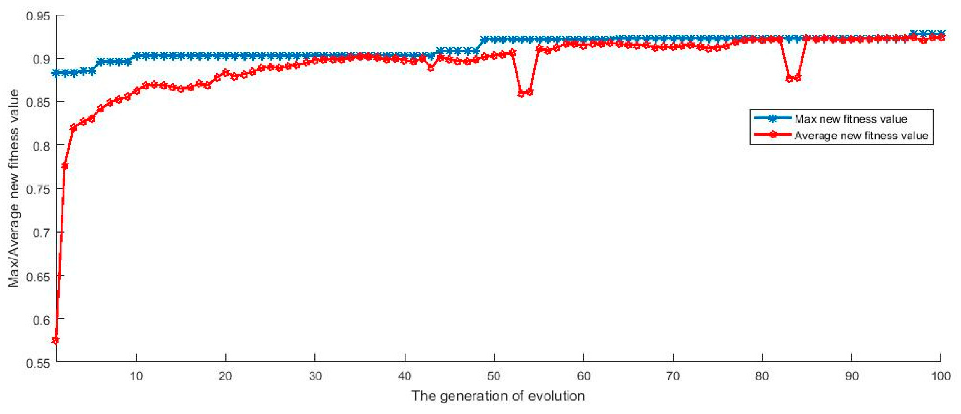
2.3. Optimization Results of Detection Platform by Using Genetic Algorithm

By optimizing the detection platform with Genetic Algorithm, after 100 generations of evolution, the optimized main variables (current intensity I, coil distance L, coil turns N) and performance indexes (magnetic flux density, Bx component of magnetic flux density, uniformity of magnetic flux density, uniformity of Bx component of magnetic flux density) of the detection platform can be obtained. Considering the differences in the standards for the elimination of dimensionality in the process of calculating the fitness value of individuals in different generations, the standards containing all the individual performance data in the evolution of 100 generations are now uniformly used to compare the highest new fitness value of each generation. Figure 5 shows the optimization process of each generation through Genetic Algorithm.
Figure 5 demonstrates that with the continuous evolution of each generation, both the maximum new fitness value and the average new fitness value keep improving and gradually converge. Owing to the influence of the penalty function of Genetic Algorithm, the fitness values of individuals whose magnetic flux density did not meet the constraint conditions in the 52–53 and 82–83 generations were reduced, which was reflected in their average new fitness values.
Table 3 and Table 4 show that the individual with the maximum new fitness value was used as the standard to compare the detection platform variables and the detection platform performance between the detection platform before optimization of Genetic Algorithm and the detection platform after optimization of Genetic Algorithm. Before and after optimization, the magnetic flux density of the detection platform increased from 17.2111 (Gs) to 19.3294 (Gs), the Bx component of magnetic flux density decreased from 1.3583 × 10⁻¹⁰ (T) to 4.8775 × 10⁻¹¹ (T), the uniformity of the magnetic flux density decreased from 0.0028 to 3.7008 × 10⁻⁴, and the uniformity of the Bx component of magnetic flux density decreased from 1.9896 × 10⁻¹¹ to 1.1209 × 10⁻¹¹, which meets the optimization requirements of improving the magnetic flux density, reducing the Bx component of magnetic flux density, reducing the uniformity of the magnetic flux density and the uniformity of the Bx component of magnetic flux density, thus proving that the detection platform has highly optimized and accurate performance.
Owing to the use of elitist preservation strategy, the optimal individual of each generation was saved for the next generation, and the optimal individual of the n-th generation was the optimal individual of all the population individuals of the 1-n generation including the initial population. Therefore, the optimal individual of the 100th generation is the optimal individual obtained in the entire evolution process, and the detection platform parameters and performance parameters of the detection platform listed in Table 4 are taken as the basis for the subsequent selection of MNPs detection positions and establishment of MNPs measurement models.

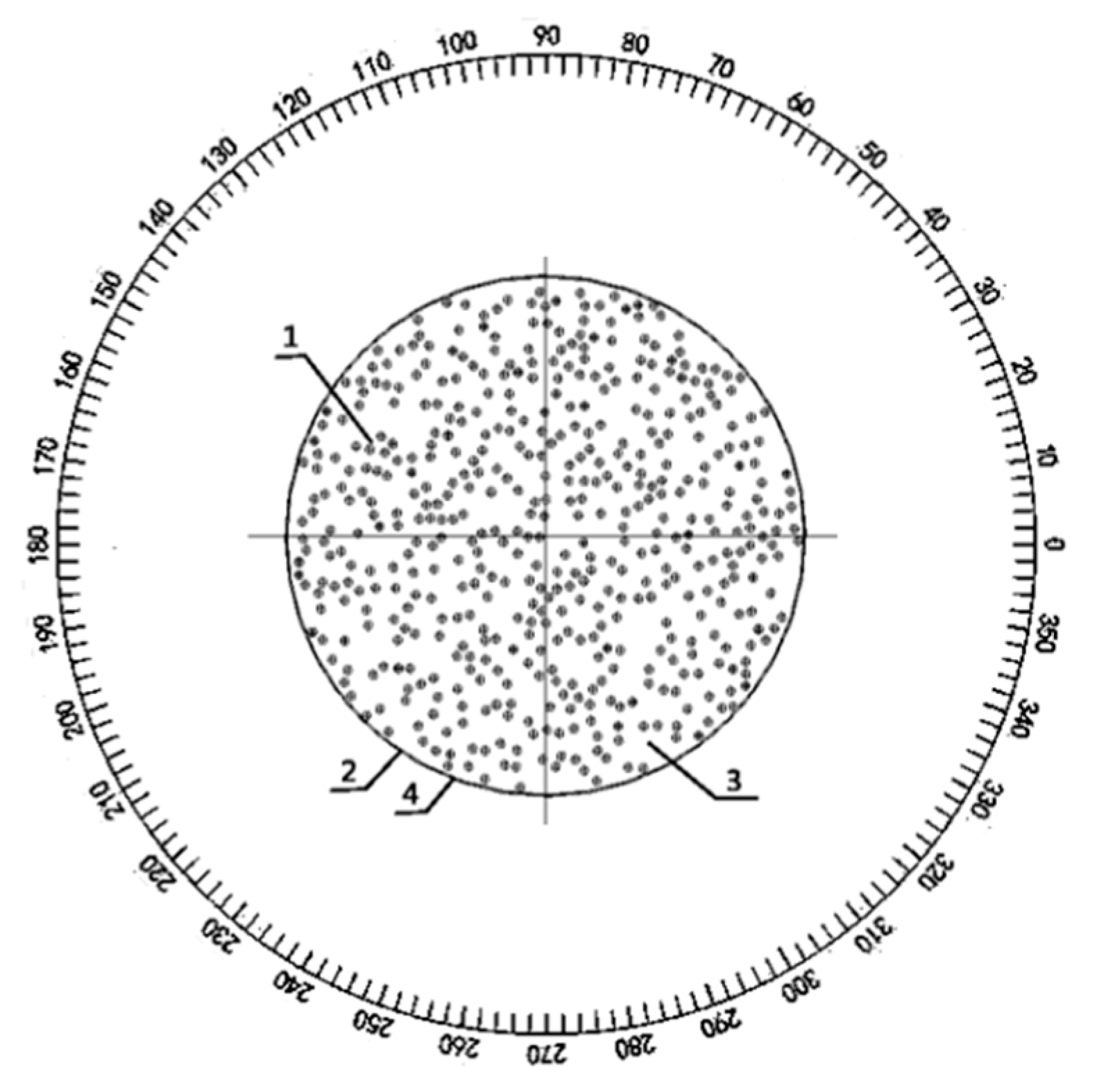
3. Decision of MNPs Detection Positions

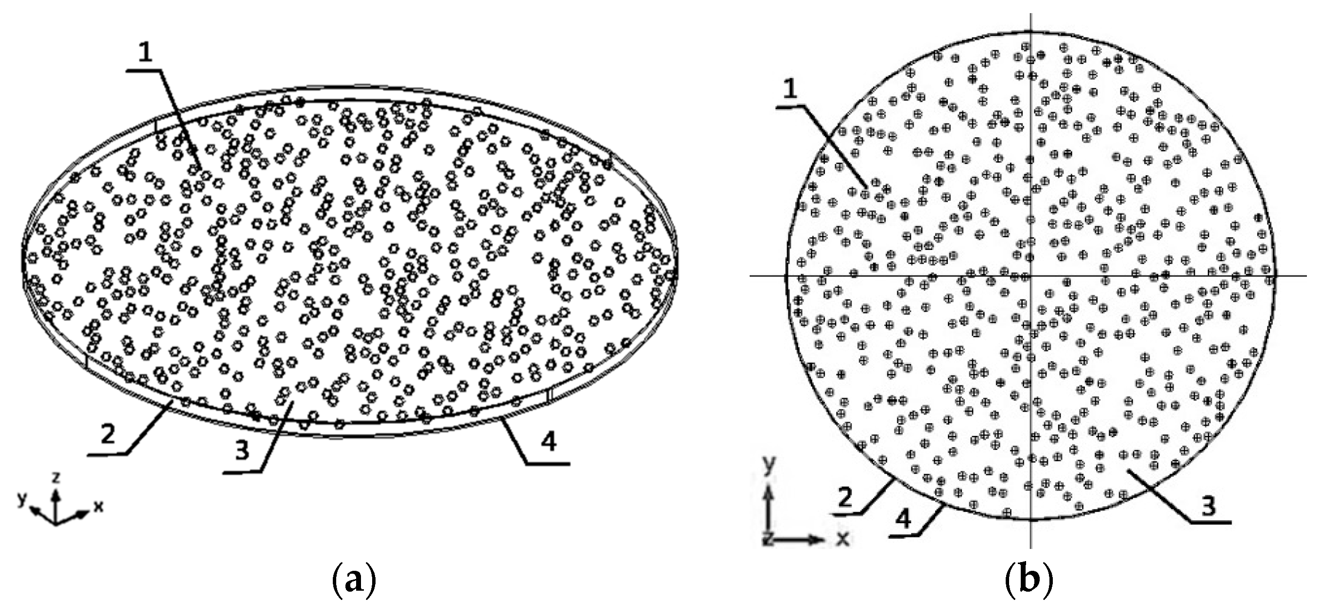
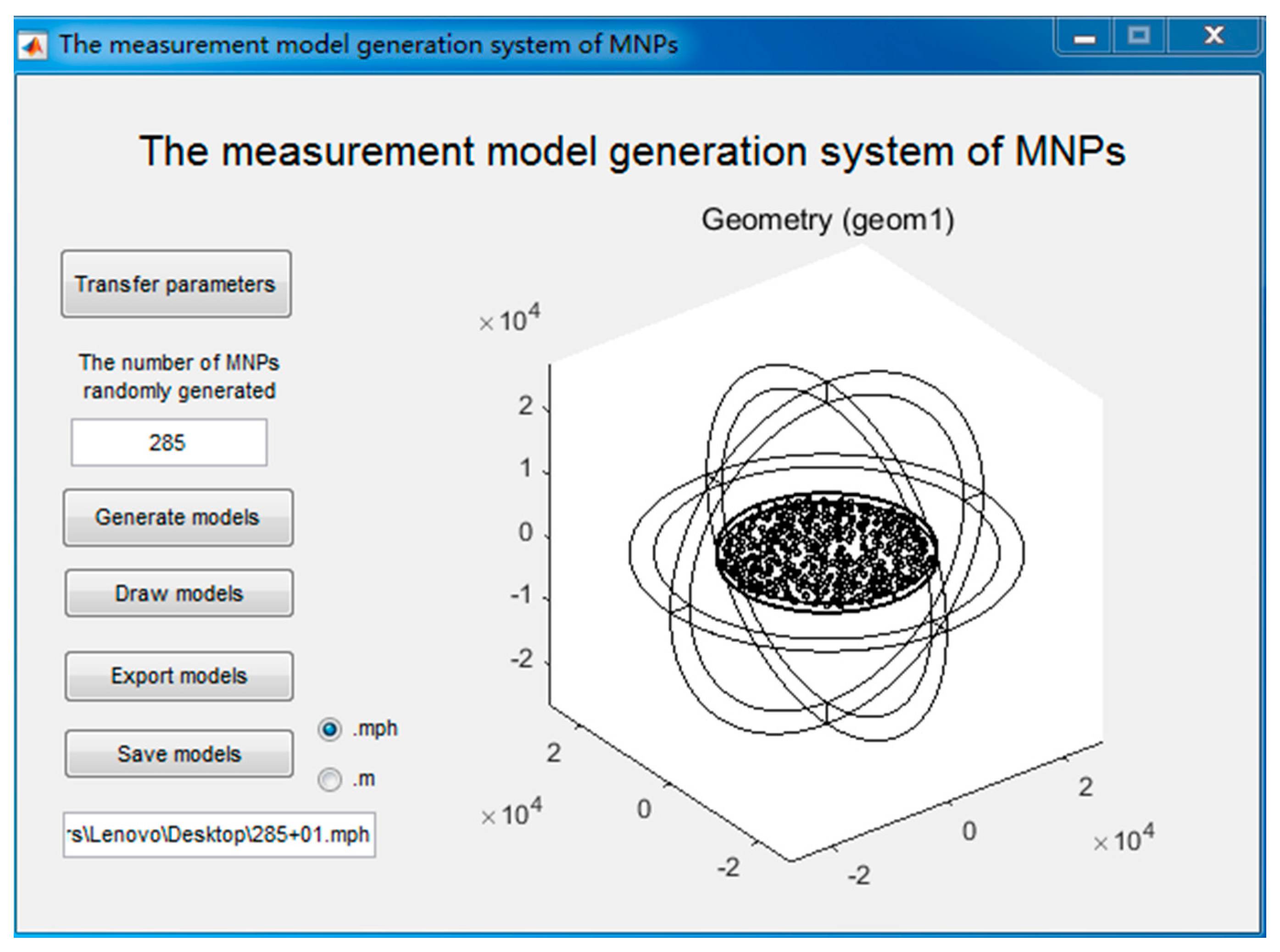
3.1. Generation and Preservation of MNPs Measurement Models in Detection Platform

According to the optimization results of Genetic Algorithm, the parameters of the detection platform were set as input current intensity I = 2.75 (A), coil distance L = 0.1771 (m), coil turns 300, and the four performance indexes are as follows: Magnetic flux density equals 19.3294 (Gs), Bx component of magnetic flux density equals 4.8775 × 10⁻¹¹ (T), uniformity of magnetic flux density equals 3.7008 × 10⁻⁴, and uniformity of Bx component of magnetic flux density equals 1.1209 × 10⁻¹¹.
Through data transmission between MATLAB and COMSOL, parameters of MNP detection platform obtained by using Genetic Algorithm optimization are directly transferred to COMSOL. According to the properties and motion rules of MNPs used in this study, magnetic agglomeration may occur in the detection device [21,36]. Through analyzing the phenomenon of magnetic agglomeration by Cluster Moving Monte Carlo method [37,38,39], it can be concluded that the MyOne particle with a radius of 500 nm used in this study generates chain agglomeration in the MNP device, and the orientation of the magnetic moment of the particle is parallel to the applied magnetic field. In COMSOL, when the random function is used to simulate the distribution of MNPs, the above-mentioned phenomenon of magnetic agglomeration is taken into consideration. Then, by setting the number of MNPs, simulation models for the MNPs measurement can be obtained. This study designs the measurement model generation system of MNPs based on MATLAB GUI, as shown in Figure 6.

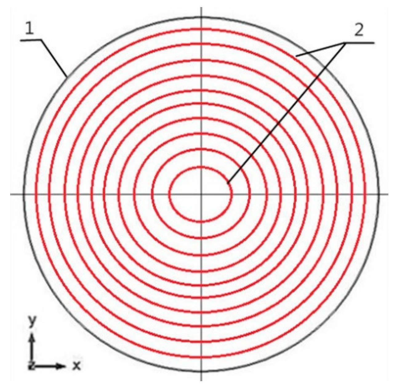
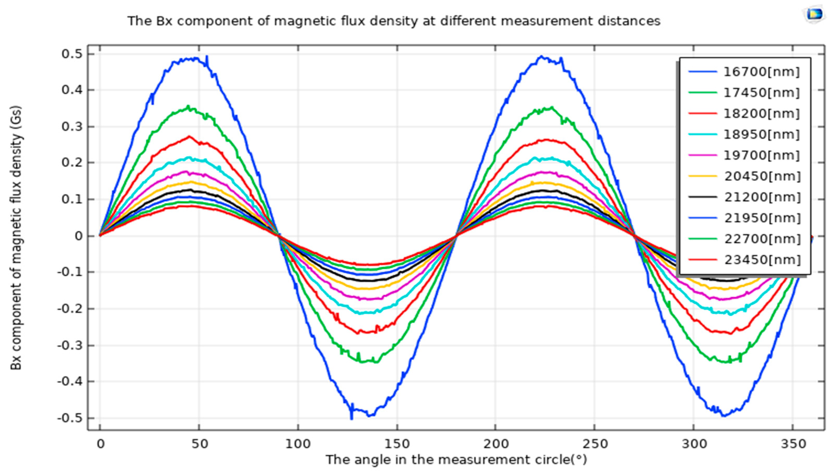
3.2. Optimization of Detection Distance of MNPs

Based on the detection platform optimized by using Genetic Algorithm, the detection positions of MNPs were selected and optimized. First, the relationship between the detection distance and the size of the MNP device was established to obtain the limit measurement number and detection distance of MNPs under the set size. In this study, according to the properties of MNPs, the number of MNPs occupying the m% cross-sectional area of the MNP device is defined as the limit measurement number N, as shown in Equation (11).
N = m % × S s 1 ,
In Equation (11), N represents the limit measurement number, m % represents the maximum proportion of the occupied area of all MNPs in the sectional area of the device that can be occupied according to the properties of MNPs and the shape of the device, S represents the cross-sectional area of the internal region of MNP device that does not include the border, and s 1 represents the cross-sectional area of a single MNP. Considering that the radius of the internal region of the MNP device was 15 μm and the radius of MyOne particle was 500 nm, the limit measurement number corresponding to this device can be obtained through Equation (11), that is, N = 405, and N can be used as the calculation basis for detection distance of MNPs, which is described in the following paragraphs.
Random function was used to simulate the distribution of MNPs in the device when the limit measurement number was reached. Ten different models were generated, and uniform magnetic field simulation experiments were conducted on these ten models. For calculation results of each model, 1000 Bx components of magnetic flux density were evenly taken at the same distance every time, and then data were transferred to MATLAB. 1000 data at the same measurement distance were taken as a group, and the stability of each group was evaluated in turn. The measurement distance which just reached the set stability index was taken as the corresponding detection distance of this model. The ten models generated were successively defined as model1–model10 and the group of data extracted at different measurement distances in each model was compared and calculated by using the corresponding group of data extracted in the reference model named Model1. The calculation method of stability evaluation is shown in Equation (12).
F i = 1 1000 j = 1 1000 | m B x j M B x j M B x j | ,
In Equation (12), F i ( i = 1 , 2 , , 10 ) represents the stability of each model in the ten models respectively, m B x j ( j = 1 , 2 , , 1000 ) represents 1000 Bx components of magnetic flux density that were evenly extracted at a certain measurement distance of the i-th model, and M B x j ( j = 1 , 2 , , 1000 ) represents the Bx component of magnetic flux density of the same position at the same measurement distance in the reference model named Model1.
The reference model called Model1 is the result obtained by simulation calculation when MNPs whose number equals the limit measurement number are uniformly distributed in the device. Considering that the internal radius of the MNP device is 15 μm, starting from 16,700 nm away from the central point of the device, 1000 Bx components of magnetic flux density were uniformly extracted from a certain measurement distance in accordance with the circular shape with step length of R/20 = 750 nm, which is shown in Figure 7.
For the ten models generated, the above-mentioned operations and calculations were carried out. These ten models were calculated by using COMSOL and the results of Bx components of magnetic flux density extracted uniformly according to the circle at a certain measurement distance are shown in Figure 8a–j.
According to the definition of stability value F i in Equation (12), when F i is smaller, stability of the model is better. With the increase of measurement distance, stability of the model is improved, but the response magnetic field intensity of the model is weakened, which affects the measurement accuracy. This study considers the measurement distance of each model as the detection distance l i ( i = 1 , 2 , , 10 ) corresponding to model1–model10 when the stability value of different measurement distances is less than 0.2 for the first time, and the detection distances l i ( i = 1 , 2 , , 10 ) corresponding to these ten models are listed in Table 5.
In combination with the results presented in Table 5, the detection distance L corresponding to the device can be determined by using Equation (13) which is represented as follows.
L = 1 10 l i , i = 1 , 2 , , 10 ,
In Equation (13), L represents the corresponding detection distance of the MNP device, l i ( i = 1 , 2 , , 10 ) represents the detection distances of ten models obtained from stability evaluation. According to Equation (13) and the results in Table 5, the corresponding detection distance of the MNP device is L = 20,525 ( n m ) .

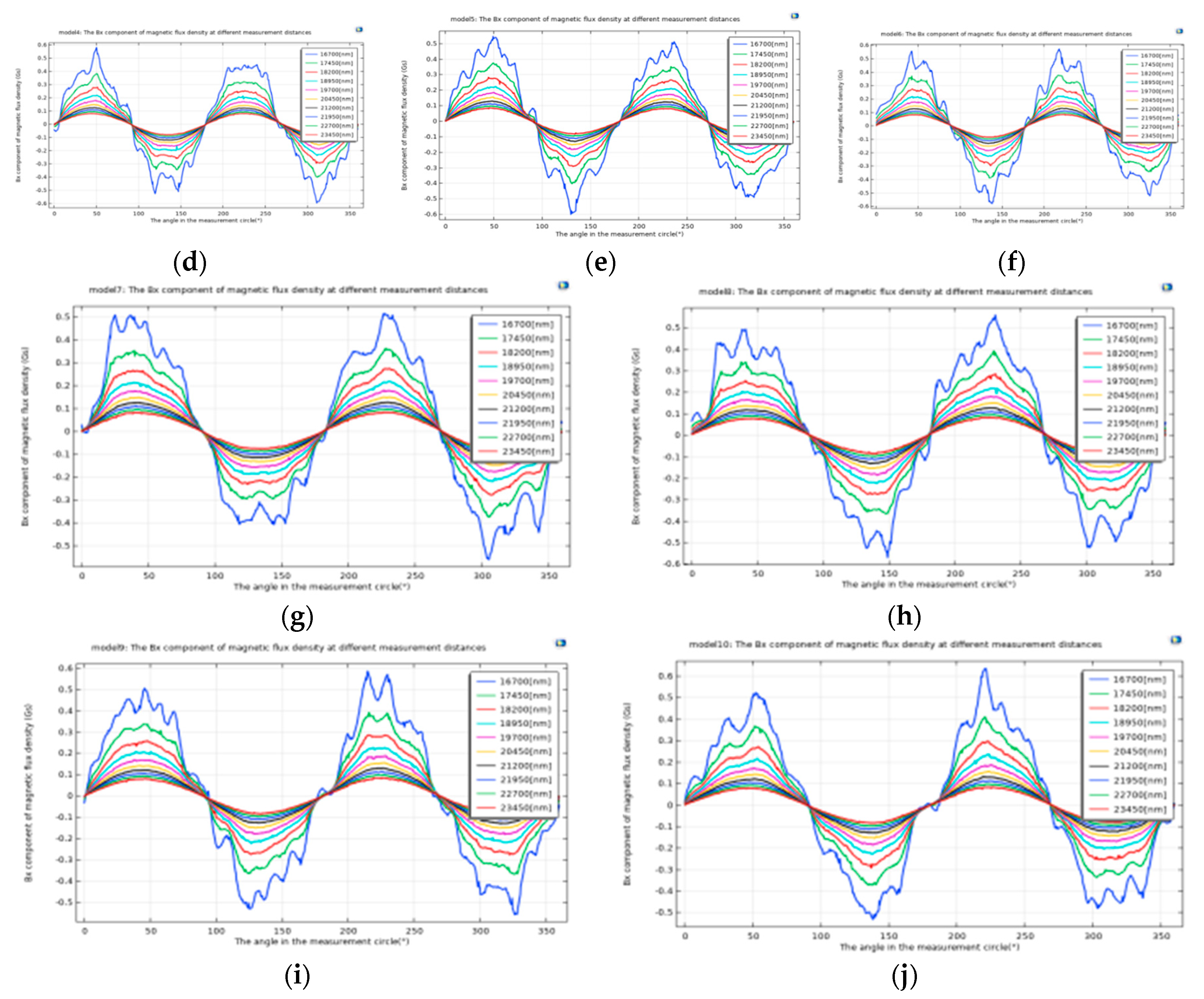
3.3. Establishment of MNPs Measurement Models at Different Detection Positions

3.3.1. Establishment of Sample Sets Corresponding to Different Detection Positions

Based on the known detection distance L = 20,525 ( n m ) , MNP devices with different numbers of MNPs were simulated in uniform magnetic field by using COMSOL respectively; and the sample sets of machine learning (including training sets and test sets) were established by using COMSOL post-processing tool. The limit measurement number N was considered as a base for the change in the number of MNPs and n MNPs were reduced successively in each group of experiments, where n equals the integer part of N/20 and n = 20 can be obtained through calculation. In one set of experiments, ten different models with the same number of MNPs were generated by using the random function. A total of ten sets of experiments were conducted, including 100 simulation models of MNP devices. Taking the detection distance L as the radius, 360 Bx components of magnetic flux density were extracted uniformly by using COMSOL post-processing tool. The above-mentioned operations were performed on the 100 simulation models of MNP devices to establish the sample sets of machine learning, of which 70% was the training sets and 30% was the test sets.
Corresponding to the positions where the 360 Bx components of magnetic flux density were uniformly extracted from each model, the 360 detection positions were reasonably divided into 90 groups (every four symmetrical positions were regarded as a group, e.g., one group for the positions of serial numbers 30, 150, 210, and 330, and one group for the positions of serial numbers 45, 135, 225, and 315). Schematic illustration of 360 detection positions of the MNP device is shown in Figure 9.
Based on different groups, the established sample sets were divided according to the positions of groups 1–90 (Position1–Position90), and 90 sample sets corresponding to the grouping positions were established (including training sets and test sets).

3.3.2. Establishment of MNPs Measurement Models through Simulated Annealing Neural Network

For each group of positions in groups 1–90 (Position1–Position90), the training set of the corresponding sample set was used to train the neural network model, in which the Bx components of magnetic flux density of the four symmetric positions were taken as the four inputs of the neural network, and the number of MNPs was taken as the output. The training sets corresponding to positions in groups 1–90 were arranged into sample vectors suitable for neural network training format. The input and output data were normalized through the mapminmax function in MATLAB to meet the requirements of neural network model [40]. In this study, number of neurons in the hidden layer was 10, and that in the output layer was 1.
The sim function in MATLAB is used to calculate and simulate, and the training data are input to obtain relevant results. The above-mentioned results were inversely normalized to obtain the corresponding fitting data. The input data of the training set and the test set corresponding to the positions of this group were normalized, which was combined with the established neural network model through the sim function to predict the output data (the number of MNPs). The above-mentioned prediction results were compared with the true data to calculate the mean absolute error (MAE) [41] and detection accuracy of MNPs number. In this paper, MAE was mainly used to evaluate the fitting effect of the established model on samples in the training set, while the detection accuracy of MNPs number was used to measure the prediction effect on samples in the test set. The calculation methods are represented in Equations (14) and (15), respectively.
M A E = 1 M 1 M | x i X i | ,
In Equation (14), M A E is the mean absolute error at different detection positions, M is the number of samples in the training set, x i is the predicted value of the model, and X i is the true number of MNPs.
A = 1 M i = 1 M ( 1 | P T T | ) ,
In Equation (15), A represents the detection accuracy of MNPs number in the group (a group in the group 1–90), M represents the number of samples in the test set, P represents the predicted number of MNPs obtained from the neural network model, and T represents the true number of MNPs in the test set.
Considering the limitations of BP neural network structure, Simulated Annealing (SA) algorithm [42] was used to optimize the weight and threshold parameters of the neural network. After the completion of the network parameter setting of the neural network model, the parameters of the SA algorithm were initialized, setting the initial temperature Tmax = 50, the maximum annealing number Lm = 1000 and the termination temperature Tmin = 0.01 in the SA algorithm. Equation (16) was used to calculate the individual fitness value S in the SA algorithm.
S = i = 1 k | Y i Z i | ,
In Equation (16), S represents individual fitness value, k represents the number of samples in training set p1, Y i represents the predicted value of the i-th sample in the training set p1 through the neural network reconstructed and retrained with the new solutions of weights and thresholds, and Z i represents the true value of the i-th sample in the training set p1.
Increment of the fitness value of the new individual relative to that of the previous individual was calculated. The increment c < 0 indicates that the error decreases, thus the new solution should be retained and the SA temperature t should be reduced to 0.95 t. When the increment c 0 , the random variable is added and Equation (17) is used to make judgments.
R = exp ( c t ) ,
In Equation (17), c represents the increment of the fitness value of the new individual relative to that of the previous individual and t represents the simulated annealing temperature at this time. When r a n d < R , the new solution was retained and the SA temperature was reduced from t to 0.99 t. When c 0 and r a n d R , the new solution was discarded and the SA temperature was increased from t to 1.01 t.
The above-mentioned process of generating new solutions and changing annealing temperature was repeated, and the weights and thresholds of the neural network were constantly optimized. The SA temperature was changed correspondingly according to the individual fitness value of the new solution. Owing to the use of random variables in the process of judging whether the new solution is retained or not, the SA process has certain probability to jump out of local optimization and realize global optimization. When the SA temperature decreases to less than termination temperature Tmin = 0.01, or the maximum annealing number Lm = 1000 is reached, the SA process ends. Finally, the optimal SA results are assigned to the weights and thresholds of the neural network to optimize the neural network, and the SA neural network model of MNPs corresponding to the detection positions is obtained.
Taking the 20th group of positions in the group 1–90 as an example, the prediction effect of the neural network model before and after optimization of SA algorithm was compared, as shown in Figure 10.

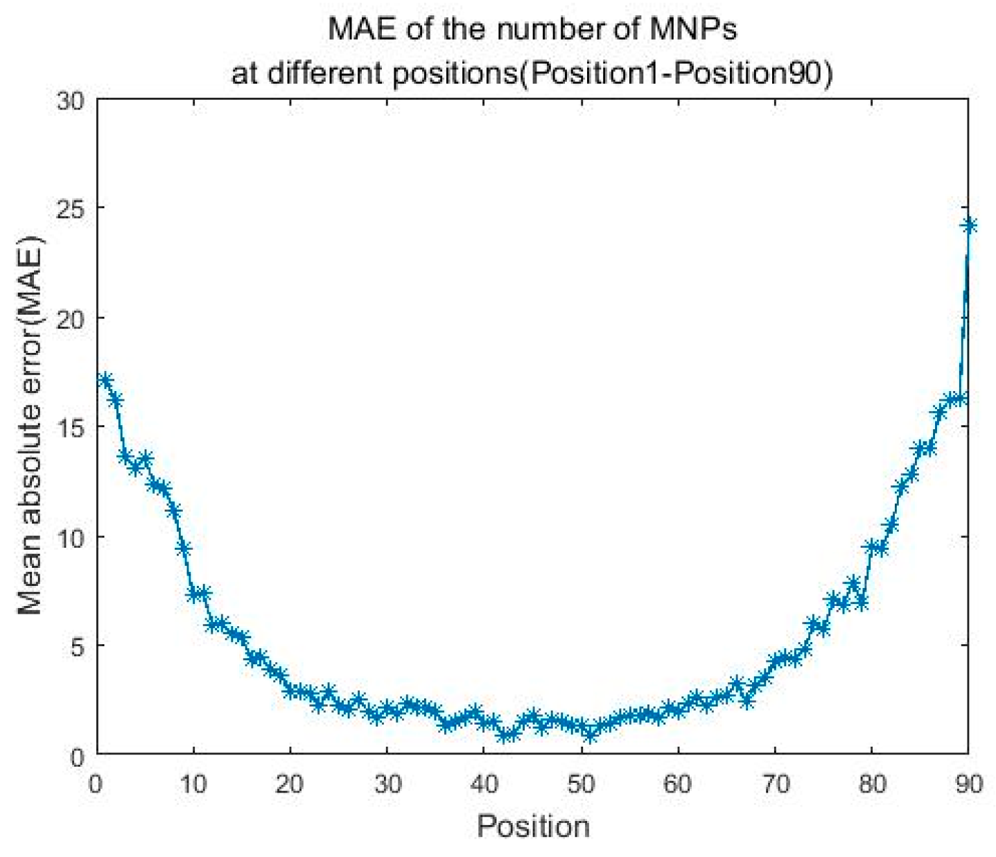
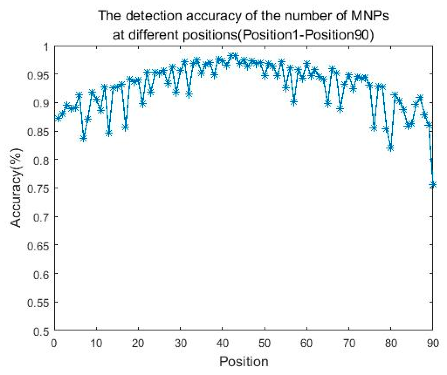
3.4. Construction of the Detection Positions Evaluation Function

According to the requirements of measuring the number of MNPs and the actual performance of the magnetic sensors, MAE, detection accuracy of the number of MNPs and average response magnetic field intensity were considered as the main indexes to evaluate whether the detection positions were appropriate or not. For the detection positions of group 1–90 (Position1–Position90), the evaluation value of the group was greater when the MAE was smaller, the detection accuracy of the number of MNPs was higher and the average response magnetic field intensity was also higher. Based on the obtained MAE, detection accuracy of the number of MNPs and average response magnetic field intensity, combined with the linear weighting method, the evaluation function H ( x ) was constructed, which is shown in Equation (18).
max H ( x ) = i = 1 m w i f i ( x ) ,
In Equation (18), m represents the number of index functions, w i represents the weighting factor, f i ( x ) represents the index function, and H ( x ) represents the evaluation function.
Through the evaluation function H ( x ) , the detection positions of groups 1–90 are evaluated and sorted according to the evaluation value, so as to obtain the optimal detection position. Moreover, MATLAB GUI [43] is used to process and display the ranking of the top ten groups of positions which have the greatest evaluation values in groups 1–90 and the specific information of the four symmetric positions contained in each group of the top ten positions, which is shown in Figure 11.
Response magnetic field intensity and average response magnetic field intensity of each group of positions were calculated and compared by using Equations (19) and (20).
B i j = 1 4 n ( j = 1 n ( | B i j 1 | + | B i j 2 | + | B i j 3 | + | B i j 4 | ) i = 1 , 2 , , 90 ,   j = 1 , 2 , , 10 ,
In Equation (19), B i j ( i = 1 , 2 , , 90 ,   j = 1 , 2 , , 10 ) represents the response magnetic field intensity corresponding to the j - th number of MNPs in the i - th group of positions, n represents the number of samples corresponding to the j - th number of MNPs in the training set of the i - th group of positions, and B i j 1 , B i j 2 , B i j 3 , B i j 4 represent the Bx components of magnetic flux density at four positions of each sample corresponding to the j - th number of MNPs in the training set of the i - th group of positions.
B i = 1 10 j = 1 10 ( B i j ) i = 1 , 2 , , 90 ,
In Equation (20), B i ( i = 1 , 2 , , 90 ) represents average response magnetic field intensity of the i - th group of positions, B i j ( i = 1 , 2 , , 90 ,   j = 1 , 2 , , 10 ) represents the response magnetic field intensity corresponding to the j - th number of MNPs in the i - th group of positions, which is defined in Equation (19), and j = 1 , 2 , , 10 represent 10 different types of number of MNPs.

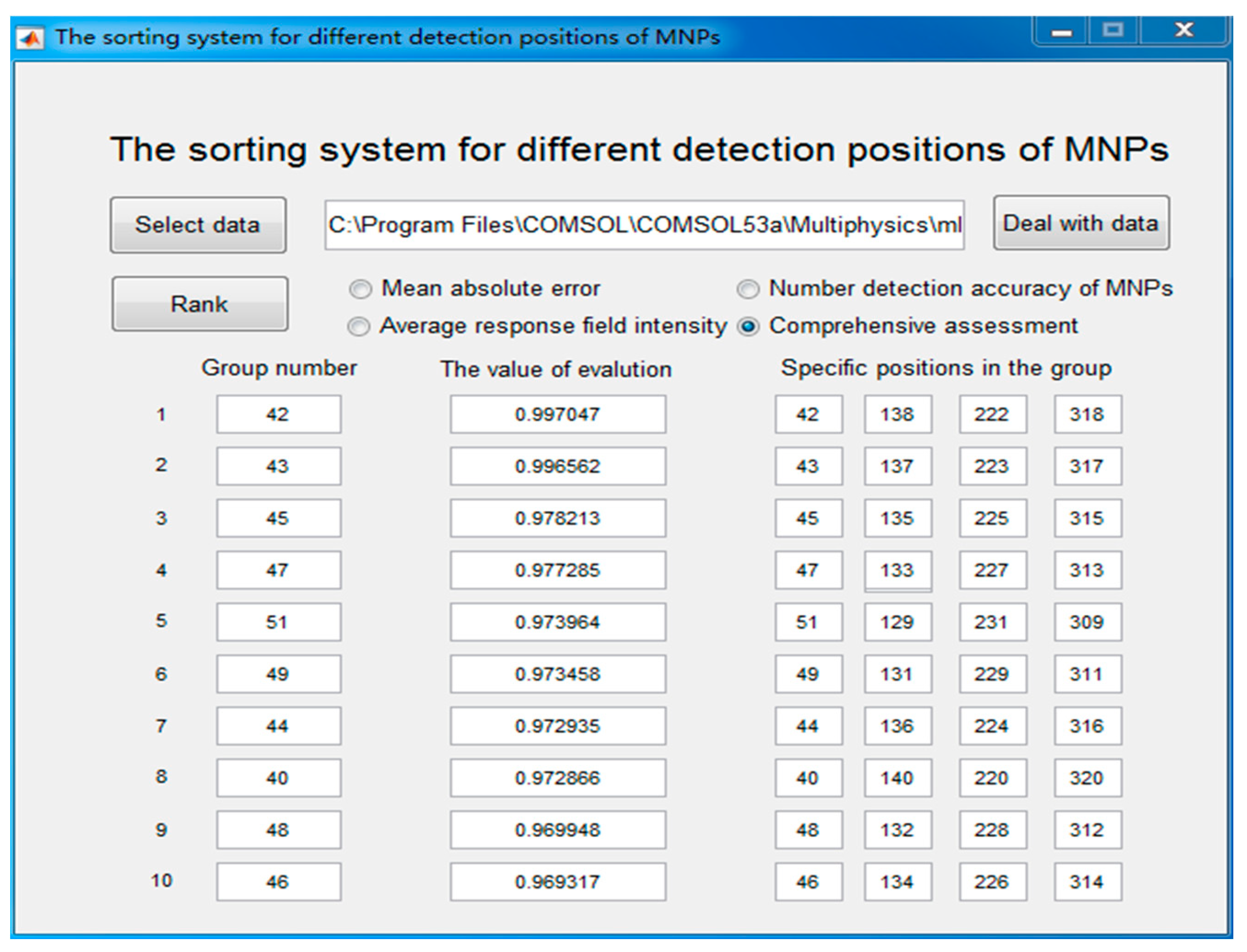
3.5. Obtaining of the Optimal Detection Positions

For groups 1–90, the MAE, the detection accuracy of the number of MNPs and the response magnetic field intensity are shown in Figure 12, Figure 13 and Figure 14, respectively.
Table 6 summarizes the ranking of the top ten groups of positions with the greatest evaluation values in Position1–Position90 and the specific information of the four symmetric positions contained in each group of the top ten groups. According to the evaluation values, the positions in the 42nd group (Position42, including four symmetric positions of 42, 138, 222, and 318) rank first in all groups of positions, which has the greatest evaluation value and is regarded as the optimal detection position. The four symmetric positions in Position42 and the corresponding sample sets are selected for the establishment and comparison of the MNPs number detection models.

4. Establishment and Comparison of MNPs Number Detection Models

According to the discussion in Section 3, the optimal group of detection positions is Position42 (as shown in Figure 9, Position42 includes four symmetric positions of 42, 138, 222, and 318). The sample sets corresponding to Position42 (sample sets are discussed in Section 3.3.1, including training sets and test sets) are used to establish and compare different MNPs number detection models. The sample sets contain 10 types of samples with different numbers of MNPs and each type of samples has 10 samples with different distribution of MNPs. The specific composition of the sample sets are listed in Table 7.
In this study, the sample sets corresponding to the optimal detection positions (Position42) were used to, respectively, establish MNPs number detection model based on RBF Neural Network, MNPs number detection model based on Simulated Annealing Neural Network, and MNPs number detection model based on PLS multivariate regression analysis. The above-mentioned three MNPs number detection models were evaluated and compared according to MNPs number detection accuracy, MAE, and root mean square error (RMSE) [44]. Among the three evaluation indexes, the calculation methods of the MAE and the detection accuracy of MNPs number are, respectively, discussed in terms of Equations (14) and (15) in Section 3.3.2.

4.1. MNPs Number Detection Model Based on RBF Neural Network

Based on the optimal detection positions (Position42) and the sample sets corresponding to the optimal detection positions (presented in Table 7), RBF neural network was trained and used to establish the MNPs number detection model. RBFNN model [45] has the advantages including optimal approximation, simple training, rapid learning convergence, and overcoming local minimum, and to some extent, it solves the local optimal problem existing in ordinary BP neural network.
As a feedforward neural network, the RBF neural network in this study is set as four inputs (namely the four Bx components of magnetic flux density (Bx1, Bx2, Bx3, Bx4) at the optimal detection position), one output (namely the number of MNPs), and ten hidden layer nodes determined according to the optimization results. In the process of training RBF neural network, this study selects Gaussian function as the activation function of the network and adopts K-means clustering algorithm [46] to determine the center position of RBF.
After determining the center position of RBF, connection weights can be obtained according to the Least Square method [47], as shown in Equation (21), where N represents the number of samples, m represents the number of nodes in the hidden layer which is 10 in this study, and c max denotes the maximum distance between the centers.
w = exp ( m c max x n c i ) n = 1 , 2 , , N , i = 1 , 2 , .. , m ,
The RBF neural network was trained with the sample sets corresponding to the optimal detection position (70 samples in the training set and 30 samples in the test set), and finally the MNPs number detection model based on RBF neural network was established. The prediction results of the model for the training set and the test set are shown in Figure 15. The MAE of this model is 11.3953, the MNPs number detection accuracy is 0.9647, the predicted RMSE of the training set is 13.9393, and the predicted RMSE of the test set is 13.1770. Figure 15 indicates that this model has certain error when the number of MNPs is small. Moreover, it generally shows a good quantitative detection effect.

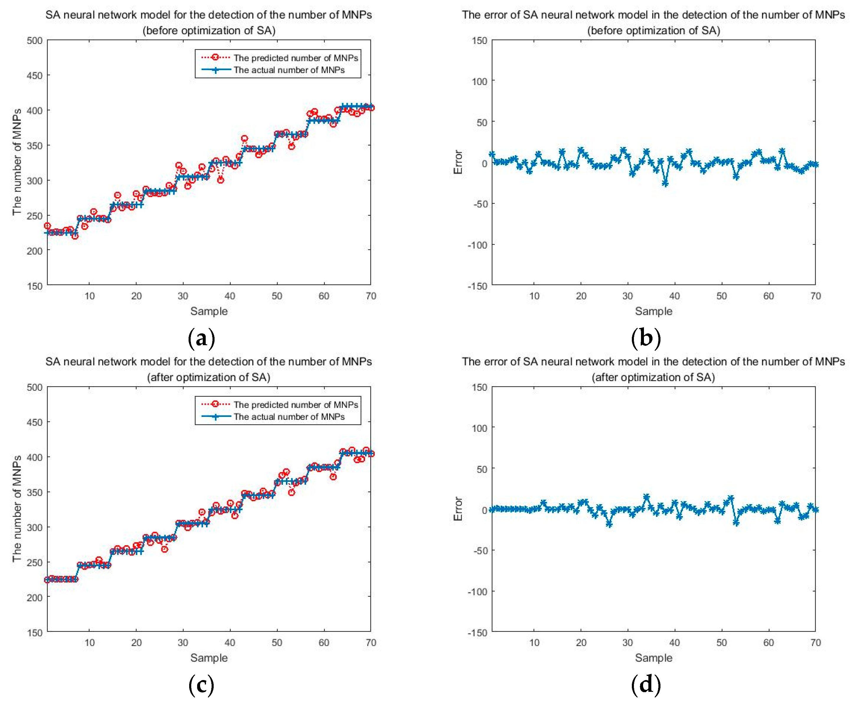
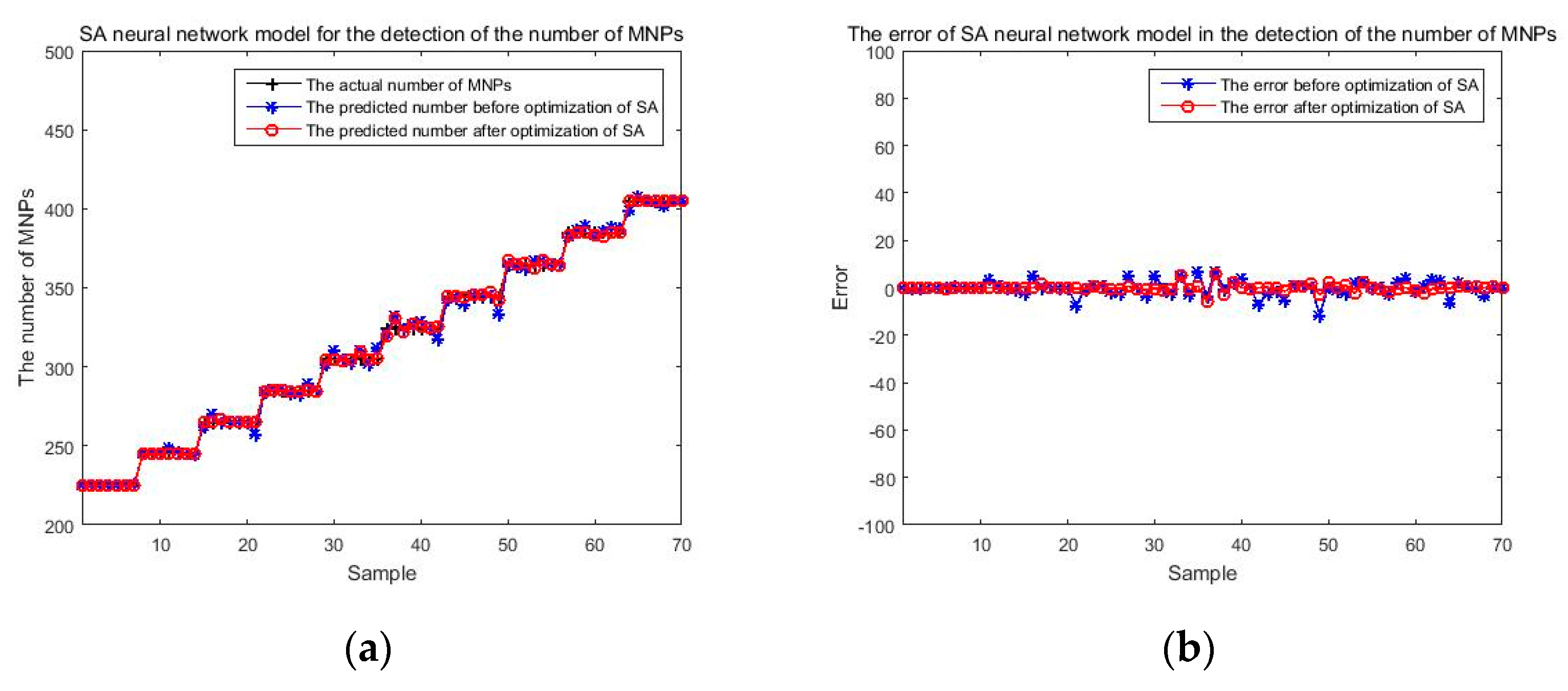
4.2. MNPs Number Detection Model Based on Simulated Annealing Neural Network

According to the optimal detection position determined in Section 3 (Position42), the sample set corresponding to this group of positions was used to establish the MNPs number detection model based on SA neural network.
This model is a 4-10-1 neural network model (the four Bx components of magnetic flux density at the optimal detection positions are the input, and the number of MNPs is the output), which utilizes the global optimization ability of SA algorithm, overcomes the problem of local optimization caused by gradient descent method in common BP neural network, and avoids the randomness of weight selection in common BP neural network, in order to effectively improve the prediction accuracy of neural network model. Partial comparison results between the true values of the number of MNPs and the predicted values of this model are presented in Table 8.
Figure 16 shows the prediction results and prediction errors of this model for training samples before and after SA optimization. The model after SA optimization (marked in red in the figure) performs significantly better than the model before SA optimization (marked in blue in the figure) in prediction effect. Moreover, the prediction results of the model after SA optimization are much closer to the true values (marked in black in the figure), thus the detection effect of the number of MNPs in the optimized model gets significantly improved. After the optimization of SA, the MAE of this model was reduced from 2.1767 to 0.8545, and the detection accuracy of the number of MNPs was improved from 0.9711 to 0.9822.
The prediction results of the training set and the test set in this model are shown in Figure 17. The MAE of the model is 0.8545, the MNPs number detection accuracy of the model is 0.9822, the predicted RMSE of the training set is 1.5134, and the predicted RMSE of the test set is 9.2931.
The MAE and RMSE for the training set of this model are quite small. This model has excellent nonlinear fitting ability and high prediction accuracy for the number of MNPs. This model performs significantly better in all three evaluation indexes used in this study (MAE, MNPs number detection accuracy, and RMSE) than the MNPs number detection model based on RBF neural network discussed in Section 4.1. Thus it can be concluded that the SA neural network model has better MNPs detection effect and greater practical application potential.

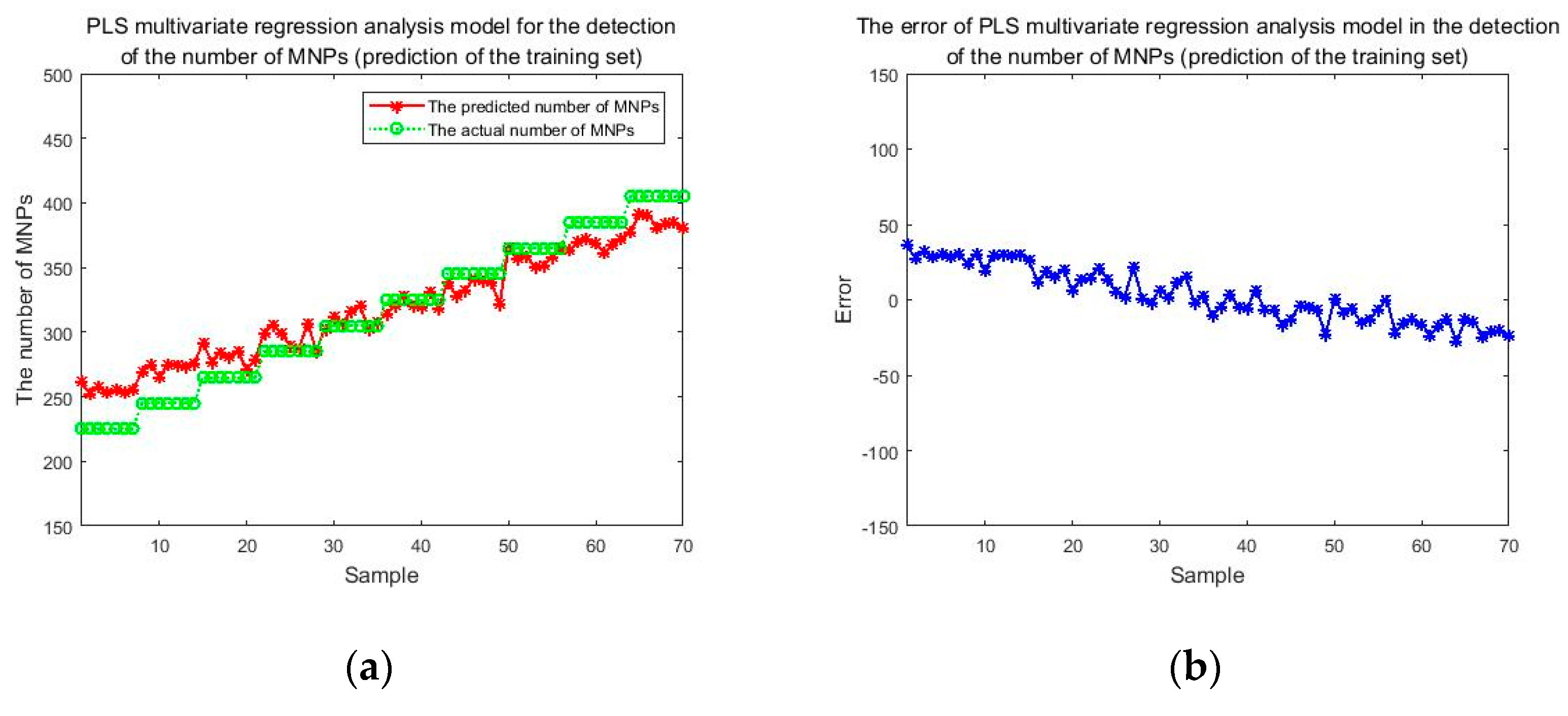
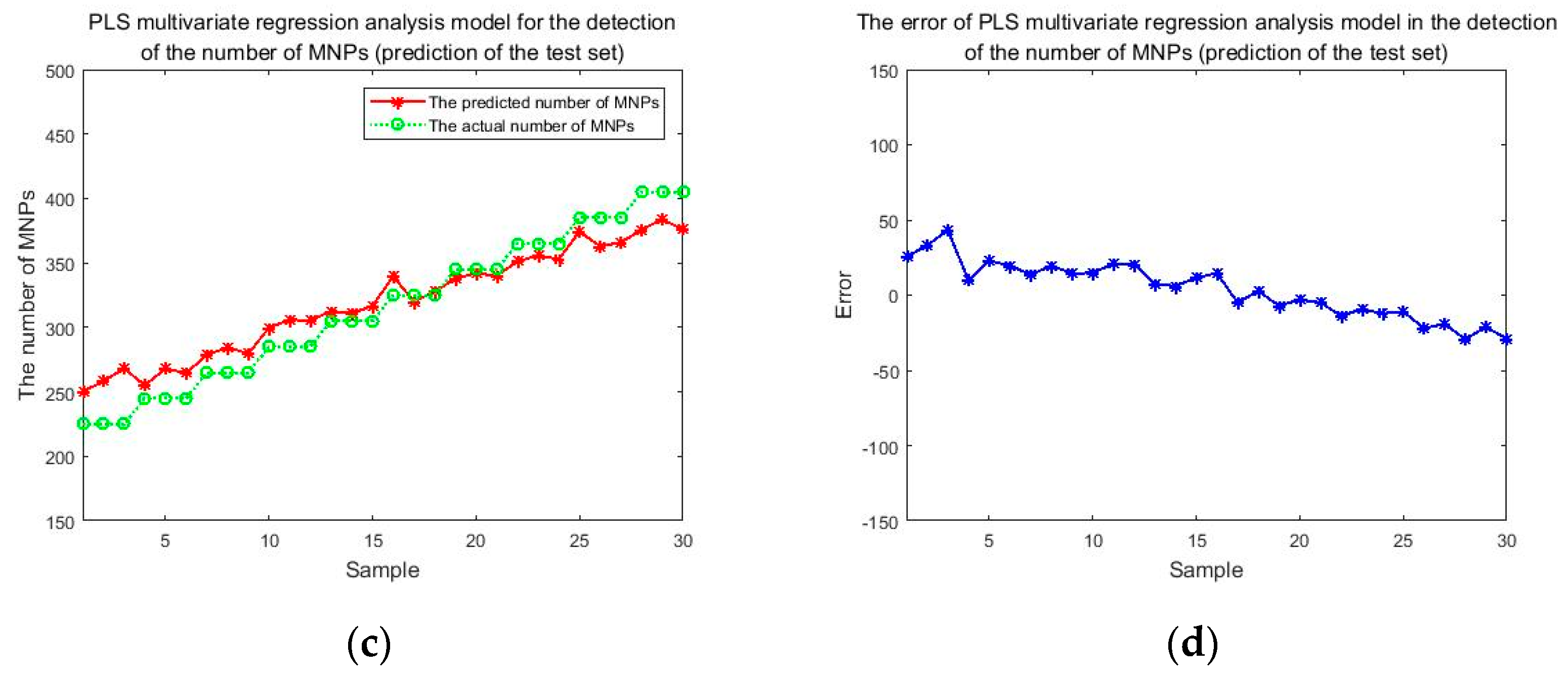
4.3. MNPs Number Detection Model Based on PLS Multivariate Regression Analysis

For comparison, the same training sample data corresponding to the optimal detection position (Position42) were used to perform partial least squares (PLS) multivariate regression analysis [48] on the number of MNPs.
The expression of the PLS regression equation [49] is represented as Equation (22).
y k = α k 1 x 1 + α k 2 x 2 + + α k p x p + F k k = 1 , 2 , , q ,
In Equation (22), q represents the number of dependent variables, F k represents the k-th column of the residual matrix F , and α k 1 , α k 2 , , α k p represent regression analysis coefficients.
In this study, four Bx components of magnetic flux density (Bx1, Bx2, Bx3, Bx4) at the optimal detection position were used as independent variables and the number of MNPs was used as the dependent variable to construct PLS multivariate regression model [50]. Finally, the regression equation can be obtained as presented in Equation (23).
y n = 128.8025 + 1035.5444 x 1 114.8877 x 2 + 379.6948 x 3 245 . 5036 x 4 ,
In Equation (23), y n represents the number of MNPs, and x 1 , x 2 , x 3 , x 4 represent the four Bx components of magnetic flux density (Bx1, Bx2, Bx3, Bx4) at the optimal detection position.
This model uses the same training set and test set of the above-mentioned RBF neural network model and SA neural network model to test the regression equation. The results indicated that the RMSE of the training set is 18.1921, and that of the test set is 18.7699. Partial comparison results between the predicted results and the true values are presented in Table 9.
The prediction results of this model for the training set and the test set are shown in Figure 18. The MAE of this model is 15.3111 and the MNPs number detection accuracy of this model is 0.9445. Compared to the PLS multivariate regression model constructed herein, the RBF neural network model discussed in Section 4.1 and the SA neural network model discussed in Section 4.2 have advantages in three main evaluation indexes (MAE, MNPs number detection accuracy, and RMSE) and exhibit significant improvement in the prediction accuracy.

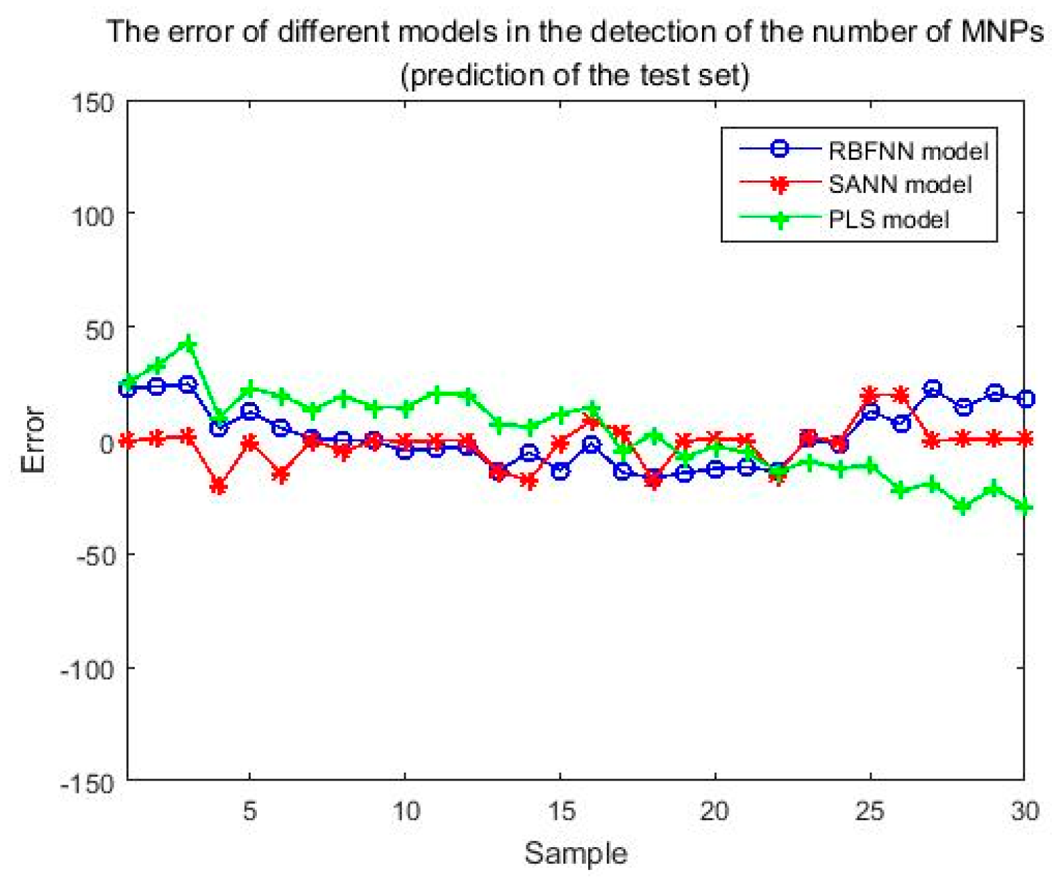
4.4. Comparison and Discussion of Different MNPs Number Detection Models

The prediction results of the three MNPs number detection models were compared and discussed. Table 10 summarizes the main evaluation index data of the three MNPs number detection models established in this study. Figure 19 and Figure 20, respectively, exhibit and compare prediction errors of training sets and test sets of different MNPs number detection models.
Table 10 and Figure 19 and Figure 20 indicate that the MNPs number detection accuracy of RBF neural network model and SA neural network model are both greater than 96%; and the MAE and RMSE of these two models are also quite small. Overall performances of the two neural network models established in this study are better than that of the PLS multivariate regression model constructed by conventional methods. It can be concluded that these two models have great prediction ability and are able to accurately detect the number of MNPs according to the weak magnetic signal at the optimal detection position.
Between the two established neural network models, SA neural network model has better performance in detecting the number of MNPs. In particular, the MAE of the SA neural network model is 0.8545, and its RMSE (training set) is 1.5134. In terms of these two evaluation indexes, the SA neural network model has obvious advantages and is far better than the other two models, with better nonlinear fitting ability and prediction effect.
To sum up, among the three MNPs number detection models established in this study, the MNPs number detection model based on SA neural network exhibits the best overall performance and can most accurately detect the number of MNPs.

5. Conclusions

This study proposes a method and device for detecting the number of magnetic nanoparticles (MNPs) based on weak magnetic signal, and applies machine learning methods to the optimization of MNP detection platform and the design of quantitative detection method. Herein, the MNP detection platform is optimized by using Genetic Algorithm, and the optimal detection platform parameters (input current intensity I, coil distance L, coil turns N) are obtained. Based on the optimal detection platform parameters, this study utilizes the Simulated Annealing Neural Network to explore the relationship between different positions of weak magnetic signals and the number of MNPs, thus establishing the sorting system for different detection positions of MNPs. According to the three evaluation indexes (mean absolute error, MNPs number detection accuracy, and average response magnetic field intensity), the comprehensive evaluation values of different detection positions are calculated and sorted to determine the optimal detection position.
In this study, based on weak magnetic signals at the optimal detection position, three different MNPs number detection models are finally established, including MNPs number detection model based on Radial Basis Function Neural Network, MNPs number detection model based on Simulated Annealing Neural Network, and MNPs number detection model based on partial least squares multivariate regression analysis. This study uses mean absolute error, MNPs number detection accuracy and root mean square error to analyze and compare the three models, and it can be concluded that all the three models can realize the detection of MNPs number. Among the three models, the MNPs number detection model based on Simulated Annealing Neural Network exhibits the best overall performance, which can accurately realize the detection of MNPs number and provide a basis for the continued study in the specific capture analyte of MNPs, with significant development potential and application prospect. Considering that the analyte in this study (hCG) is proportional to the number of MNPs, through detecting the number of MNPs in this device, contactless detection of hCG contents can be realized in short time. The technique can be extended to the contactless detection of other substances as well.

Author Contributions

L.W., T.Z. and Q.N. designed the experiments, conducted laboratory analysis, interpreted the results and wrote the manuscript; L.W., Y.H. and Z.H. revised the article.

Funding

This research was funded by Technology Support Program of Henan Province (182102210089) and the Fundamental Research Funds for the Henan Provincial Colleges and Universities in Henan University of Technology (2018XTCX02).

Acknowledgments

We extend our appreciation to the Key Laboratory fund of Henan Province for funding the work through the research project (KFJJ-2016-201).

Conflicts of Interest

The authors declare no conflict of interest.

References

  1. Beveridge, J.S.; Stephens, J.R.; Williams, M.E. The Use of Magnetic Nanoparticles in Analytical Chemistry. Annu. Rev. Anal. Chem. 2011, 4, 251–273. [Google Scholar] [CrossRef] [PubMed]
  2. Caroccia, B.; Fassina, A.; Seccia, T.M. Isolation of Human Adrenocortical Aldosterone- Producing Cells by a Novel Immunomagnetic Beads Method. Endocrinology 2010, 151, 1375–1380. [Google Scholar] [CrossRef] [PubMed]
  3. Nishiya, Y.; Hibi, T.; Oda, J.I. A purification method of the diagnostic enzyme Bacillus uricase using magnetic beads and non-specific protease. Protein Expr. Purif. 2002, 25, 426–429. [Google Scholar] [CrossRef]
  4. Yoza, B.; Arakaki, A.; Matsunaga, T. DNA extraction using bacterial magnetic particles modified with hyperbranched polyamidoamine dendrimer. J. Biotechnol. 2003, 101, 219–228. [Google Scholar] [CrossRef]
  5. Verpoorte, E.; Rooij, N.F.D. Microfluidics meets MEMS. Proc. IEEE 2003, 91, 930–953. [Google Scholar] [CrossRef] [Green Version]
  6. Gilmartin, N.; O’Kennedy, R. Nanobiotechnologies for the detection and reduction of pathogens. Chin. J. Anal. Chem. 2011, 39, 1307–1312. [Google Scholar] [CrossRef] [PubMed]
  7. Peng, J.; Xu, Y.; Wu, Y.; Chuan, N.; Gan, J.; Tian, P. Determination of E.coli with Electrochemical Impedance on Homemade Microfluidic Chip. Enzym. Microb. Technol. 2012, 50, 87–95. [Google Scholar]
  8. Simmonds, M.B. Method and Apparatus for Making Quantitave Measurements of Localized Accumulations of Magnetic Particles. U.S. Patent 6,046,585, 4 April 2004. [Google Scholar]
  9. Kotitz, R.; Matz, H.; Trahms, L. SQUID based remanence measurements for immunoassays. IEEE Trans. Appl. Supercond. 1997, 7, 3678–3681. [Google Scholar] [CrossRef]
  10. Koh, I.; Josephson, L. Magnetic Nanoparticle Sensors. Sensors 2009, 9, 8130–8145. [Google Scholar] [CrossRef]
  11. Lee, H.; Shin, T.H.; Cheon, J. Recent Developments in Magnetic Diagnostic Systems. Chem. Rev. 2015, 115, 10690–10724. [Google Scholar] [CrossRef] [Green Version]
  12. Issadore, D.; Min, C.; Liong, M. Miniature magnetic resonance system for point-of-care diagnostics. Lab Chip 2011, 11, 2282–2287. [Google Scholar] [CrossRef]
  13. Imtiaz, W.; Ghafoor, H.A.; Sehar, R. Evaluating the Performance Estimators via Machine Learning Supervised Learning Algorithms for Dataset Threshold. Int. J. Comput. Appl. 2015, 119, 1–6. [Google Scholar] [CrossRef]
  14. Sutton, R.; Barto, A.; Sehar, R. Reinforcement Learning: An Introduction (Adaptive Computation and Machine Learning). IEEE Trans. Neural Netw. 1998, 9, 1054. [Google Scholar] [CrossRef]
  15. Yan, W.; Wang, K.; Xu, H. Machine Learning Approach to Enhance the Performance of MNP-Labeled Lateral Flow Immunoassay. Nano-Micro Lett. 2019, 11, 7. [Google Scholar] [CrossRef]
  16. Khosravi, A.; Malekan, M.; Williams, M.E. Effect of the magnetic field on the heat transfer coefficient of a Fe3O4 water ferrofluid using artificial intelligence and CFD simulation. Eur. Phys. J. Plus 2019, 134, 88. [Google Scholar] [CrossRef]
  17. Min, H.; Pi-suo, C. A dynamic RBF neural network algorithm used in pattern recognition. J. Dalian Univ. Technol. 2006, 46, 746–751. [Google Scholar]
  18. Li, T.; Wang, X. Non-synchronous signal monitoring based on simulated annealing neural network. In Proceedings of the IEEE International Conference on Granular Computing, Nanchang, China, 17–19 August 2009; IEEE: Piscataway, NJ, USA, 2009. [Google Scholar]
  19. Elden, L. Partial least-squares vs. Lanczos bidiagonalization-I: Analysis of a projection method for multiple regression. Comput. Stat. Data Anal. 2004, 46, 11–31. [Google Scholar] [CrossRef]
  20. Trout, S.R. Use of Helmholtz coils for magnetic measurements. IEEE Trans. Magn. 1988, 24, 2108–2111. [Google Scholar] [CrossRef]
  21. Feng, Y. Simulation and Experimental Research on the Aggregation Performance of Magnetic Particles under Magnetic Field; Huazhong University of Science and Technology: Wuhan, China, 2016. [Google Scholar]
  22. Khashan, S.A.; Furlani, E.P. Coupled particle-fluid transport and magnetic separation in microfluidic systems with passive magnetic functionality. J. Phys. D Appl. Phys. 2013, 46, 125002. [Google Scholar] [CrossRef]
  23. Udy, J.; Hansen, B.; Maddux, S.; Petersen, D.; Heilner, S.; Stevens, K.; Lignell, D.; Hedengren, J.D. Review of field development optimization of waterflooding, eor, and well placement focusing on history matching and optimization algorithms. Processes 2017, 5, 34. [Google Scholar]
  24. Osyczka, A.; Kundu, S. A New Method to Solve Generalized Multcriteria Optimization Problems Using the Simple Genetic Algorithm. Struct. Multidiscip. Optim. 1995, 10, 94–99. [Google Scholar] [CrossRef]
  25. Vose, M.D. The Simple Genetic Algorithm: Foundations and Theory; MIT Press: Cambridge, MA, USA, 1999. [Google Scholar]
  26. Chen, T.Y.; Chen, C.J. IMPROVEMENTS OF SIMPLE GENETIC ALGORITHM IN STRUCTURAL DESIGN. Int. J. Numer. Methods Eng. 2015, 40, 1323–1334. [Google Scholar] [CrossRef]
  27. Ha, Y.H.; Han, B.H.; Lee, S.Y. Magnetic propulsion of a magnetic device using three square-Helmholtz coils and a square-Maxwell coil. Med. Biol. Eng. Comput. 2010, 48, 139–145. [Google Scholar] [CrossRef] [PubMed]
  28. Jiang, B.C.; Wang, C.C.; Liu, H.C. Liquid crystal display surface uniformity defect inspection using analysis of variance and exponentially weighted moving average techniques. Int. J. Prod. Res. 2005, 43, 67–80. [Google Scholar] [CrossRef]
  29. Zhang, D.H.; Ren, B.; Liu, S. Discuss on Evaluation of Film Cooling Uniformity. Turbine Technol. 2013, 55, 171–174. [Google Scholar]
  30. Mishra, S. Weighting method for bi-level linear fractional programming problems. Eur. J. Oper. Res. 2007, 183, 296–302. [Google Scholar] [CrossRef]
  31. Dixon, P.; Just, M.A. Normalization of irrelevant dimensions in stimulus comparisons. J. Exp. Psychol. Hum. Percept. Perform. 1978, 4, 36–46. [Google Scholar] [CrossRef]
  32. Gréwal, G.; Coros, S. Comparing a genetic algorithm penalty function and repair heuristic in the DSP application domain. In Proceedings of the Iasted International Conference on Artificial Intelligence & Applications, Innsbruck, Austria, 13–16 February 2006. [Google Scholar]
  33. Kaya, M. The effects of a new selection operator on the performance of a genetic algorithm. Appl. Math. Comput. 2011, 217, 7669–7678. [Google Scholar] [CrossRef]
  34. Liang, Y.; Leung, K.S. Genetic Algorithm with adaptive elitist-population strategies for multimodal function optimization. Appl. Soft Comput. 2011, 11, 2017–2034. [Google Scholar] [CrossRef]
  35. Min, H.; Zhuo, W.; Linghui, H. The Study of Optimizing of Physical Distribution Routing Problem System with Time Windows Based on Genetic Algorithm. In Proceedings of the 2010 International Forum on Information Technology and Applications, Kunming, China, 16–18 July 2010. [Google Scholar]
  36. Li, X.; Yao, K. The cluster-moving Monte Carlo method simulates the aggregation behavior of magnetic nanoparticles under uniform magnetic field. In Proceedings of the Second National Forum on Complex Dynamical Networks, Beijing, China, 16–19 October 2005. [Google Scholar]
  37. Satoh, A. A new technique for metropolis Monte Carlo simulation to capture aggregate structures of fine particles: Cluster-moving Monte Carlo algorithm. J. Colloid Interface Sci. 1992, 150, 461–472. [Google Scholar] [CrossRef]
  38. Aoshima, M.; Satoh, A. Two-dimensional Monte Carlo simulations of a colloidal dispersion composed of polydisperse ferromagnetic particles in an applied magnetic field. J. Colloid Interface Sci. 2005, 288, 475–488. [Google Scholar] [CrossRef] [PubMed]
  39. Peng, X.; Min, Y.; Ma, T.; Luo, W.; Yan, M. Two-dimensional Monte Carlo simulations of structures of a suspension comprised of magnetic and nonmagnetic particles in uniform magnetic fields. J. Magn. Magn. Mater. 2009, 321, 1221–1226. [Google Scholar] [CrossRef]
  40. Sadeghi, B.H.W. A BP-neural network predictor model for plastic injection molding process. J. Mater. Process. Technol. 2000, 103, 411–416. [Google Scholar] [CrossRef]
  41. Gazzaz, N.M.; Yusoff, M.K.; Aris, A.Z.; Juahir, H.; Ramli, M.F. Artificial neural network modeling of the water quality index for Kinta River (Malaysia) using water quality variables as predictors. Mar. Pollut. Bull. 2012, 64, 2409–2420. [Google Scholar] [CrossRef] [PubMed]
  42. Alrefaei, M.H.; Andradóttir, S. A Simulated Annealing Algorithm with Constant Temperature for Discrete Stochastic Optimization. Manag. Sci. 1995, 45, 748–764. [Google Scholar] [CrossRef]
  43. Gupta, R.; Bera, J.N.; Mitra, M. Development of an embedded system and MATLAB-based GUI for online acquisition and analysis of ECG signal. Measurement 2010, 43, 1119–1126. [Google Scholar] [CrossRef]
  44. Baruah, P.J.; Tamura, M.; Oki, K.; Nishimura, H. Neural network modeling of surface chlorophyll and sediment content in inland water from Landsat Thematic Mapper imagery using multidate spectrometer data. Proc. Spie 2002, 4488, 205–212. [Google Scholar]
  45. Yun, Z.; Quan, Z.; Caixin, S.; Shaolan, L.; Yuming, L.; Yang, S. RBF Neural Network and ANFIS-Based Short-Term Load Forecasting Approach in Real-Time Price Environment. IEEE Trans. Power Syst. 2008, 23, 853–858. [Google Scholar]
  46. Qiao, X.; Chang, W.; Zhou, S.; Lu, X. A prediction model of hard landing based on RBF neural network with K-means clustering algorithm. In Proceedings of the 2016 IEEE International Conference on Industrial Engineering and Engineering Management (IEEM), Bali, Indonesia, 4–7 December 2016. [Google Scholar]
  47. Gong, Z.W. Least-square method to priority of the fuzzy preference relations with incomplete information. Int. J. Approx. Reason. 2008, 47, 258–264. [Google Scholar] [CrossRef] [Green Version]
  48. Gil-García, C.J.; Rigol, A.; Vidal, M. Comparison of mechanistic and PLS-based regression models to predict radiocaesium distribution coefficients in soils. J. Hazard. Mater. 2011, 197, 11–18. [Google Scholar]
  49. Geladi, P.; Kowalski, B.R. Partial Least-Squares Regression: A Tutorial. Anal. Chim. Acta 1986, 185, 1–17. [Google Scholar] [CrossRef]
  50. Nandi, S.; Bagchi, M.C. Activity Prediction of Some Nontested Anticancer Compounds Using GA-Based PLS Regression Models. Chem. Biol. Drug Des. 2011, 78, 587–595. [Google Scholar] [CrossRef] [PubMed]
Figure 1. Structural illustration of magnetic nanoparticle detection platform.
Processes 07 00480 g001
Figure 2. Schematic illustration of magnetic nanoparticle device: (a) the front view, (b) the vertical view.
Processes 07 00480 g002
Figure 3. The ten circular 3D curves in MNP device.
Processes 07 00480 g003
Figure 4. The penalty function adjusts the roulette probability for individuals in the population: (a) the roulette probability before the adjustment and (b) the roulette probability after the adjustment.
Processes 07 00480 g004
Figure 5. Optimization process of each generation through Genetic Algorithm.
Processes 07 00480 g005
Figure 6. The measurement model generation system of MNPs based on MATLAB GUI.
Processes 07 00480 g006
Figure 7. The Bx component results of Model1 obtained at different measurement distances.
Processes 07 00480 g007
Figure 8. The Bx component results of model1–model10 obtained at different measurement distances: (a)–(j) the Bx component results of model1–model10, respectively.
Processes 07 00480 g008aProcesses 07 00480 g008b
Figure 9. 360 different detection positions of magnetic nanoparticle device.
Processes 07 00480 g009
Figure 10. The Comparison diagram of prediction effect of neural network model before and after the optimization of Simulated Annealing (SA): (a) MNPs measurement model through the optimization of SA (before optimization), (b) the detection error in MNPs measurement model (before optimization), (c) MNPs measurement model through the optimization of SA (after optimization), and (d) the detection error in MNPs measurement model (after optimization).
Processes 07 00480 g010
Figure 11. The sorting system for different detection positions of MNPs based on MATLAB GUI.
Processes 07 00480 g011
Figure 12. Mean absolute error (MAE) of the number of MNPs at Position1–Position90.
Processes 07 00480 g012
Figure 13. The detection accuracy of the number of MNPs at Position1–Position90.
Processes 07 00480 g013
Figure 14. Response magnetic field intensity at different positions (Position1–Position90): (a) the average response magnetic field intensity at Position1–Position90 and (b) the response magnetic field intensity at Position1–Position90 with different number of MNPs.
Processes 07 00480 g014
Figure 15. MNPs number detection model based on Radial Basis Function neural network (RBFNN): (a) the prediction results of RBFNN model for the training set, (b) the prediction error of RBFNN model for the training set, (c) the prediction results of RBFNN model for the test set, and (d) the prediction error of RBFNN model for the test set.
Processes 07 00480 g015
Figure 16. Comparison of prediction effect of SA neural network model before and after the optimization of SA: (a) comparison of prediction results of SA neural network model before and after optimization and (b) comparison of prediction error of SA neural network model before and after optimization.
Processes 07 00480 g016
Figure 17. MNPs number detection model based on SA neural network: (a) the prediction results of SA neural network model for the training set, (b) the prediction error of SA neural network model for the training set, (c) the prediction results of SA neural network model for the test set, and (d) the prediction error of SA neural network model for the test set.
Processes 07 00480 g017
Figure 18. MNPs number detection model based on PLS multivariate regression analysis: (a) the prediction results of PLS model for the training set, (b) the prediction error of PLS model for the training set, (c) the prediction results of PLS model for the test set, and (d) the prediction error of PLS model for the test set.
Processes 07 00480 g018aProcesses 07 00480 g018b
Figure 19. Comparison of the prediction errors of different MNPs number detection models (the training set).
Processes 07 00480 g019
Figure 20. Comparison of the prediction errors of different MNPs number detection models (the test set).
Processes 07 00480 g020
Table 1. Parameters of selected magnetic nanoparticles (MNPs) [21].
Type of MNPsParticle Radius (nm)Particle Density(kg·m−3)Relative Permeability
MyOne5001.8 × 1033.625
Table 2. Text documents recording the magnetic flux density and the Bx component of magnetic flux density of a certain individual in the population (5.txt was taken as an example and partial contents of 5.txt were shown).
Node Number (1–1000)Magnetic Flux Density (T)The Bx Component of Magnetic Flux Density (T)
10.00189980223712546523.639288164784647 × 10−8
20.00189980223297385823.639052640106748 × 10−8
30.00189980222880576073.638817048925243 × 10−8
40.00189980222462133773.638581400841419 × 10−8
50.00189980222042075453.638345705080822 × 10−8
60.00189980221620417753.638109970918461 × 10−8
70.00189980221197177253.6378742077567414 × 10−8
80.00189980220772370773.6376384248496674 × 10−8
90.00189980220346015063.637402631464796 × 10−8
100.00189980219918127013.637166836978104 × 10−8
Table 3. Comparison of detection platform variables before and after Genetic Algorithm optimization (the individual with maximum new fitness value).
Evolution Generation Input current Intensity I (A)Coil Distance L (m)Coil Turns NAverage New Fitness Value
Initial population2.50.17132930.5743
The 100th generation2.750.17713000.9244
Table 4. Comparison of detection platform performances before and after Genetic Algorithm optimization (the individual with maximum new fitness value).
Evolution Generation Magnetic Flux Density (Gs)Bx component
of Magnetic Flux Density (T)
Uniformity of Magnetic Flux DensityUniformity of Bx Component of Magnetic Flux DensityMaximum New Fitness Value
Initial population17.21111.3583 × 10−100.00281.9896 × 10−110.8832
The 100th generation19.32944.8775 × 10−113.7008 × 10−41.1209 × 10−110.9281
Table 5. Detection distances ( l i ( i = 1 , 2 , , 10 ) ) obtained by calculation from model1 to model10.
Model NameModel1Model2Model3Model4Model5
Detection distance (nm)
l 1 l 5
21,20021,95023,45019,70018,200
Model NameModel6Model7Model8Model9Model10
Detection distance (nm)
l 6 l 10
22,70018,20022,70018,20018,950
Table 6. Ranking of comprehensive evaluation values corresponding to Position1–Position90 and specific position information (top 10 positions).
RankingPosition Number
(Position1–90)
Specific Position
Information
Mean Absolute ErrorNumber Detection Accuracy of MNPsAverage Response Magnetic Field IntensityComprehensive
Evaluation Value
14242, 138,
222, 318
0.85450.98220.10500.997047
24343, 137,
223, 317
0.99370.98210.10530.996562
34545, 135,
225, 315
1.74830.97440.10570.978213
44747, 133,
227, 313
1.62370.97350.10540.977285
55151, 129,
231, 309
0.85060.96890.10360.973964
64949, 131,
229, 311
1.32130.96940.10480.973458
74444, 136,
224, 316
1.52790.96870.10560.972935
84040, 140,
220, 320
1.45230.97310.10390.972866
94848, 132,
228, 312
1.55880.96800.10520.969948
104646, 134,
226, 314
1.25640.96340.10560.969317
Table 7. The samples sets (training sets and test sets) corresponding to the optimal group of positions (Position42).
Sample Sets The Number of SamplesThe Number of MNPs
Training sets70225, 245, 265, 285, 305,
325, 345, 365, 385, 405
Test sets30225, 245, 265, 285, 305,
325, 345, 365, 385, 405
Table 8. Partial prediction results of the number of MNPs through the simulated annealing neural network model.
The Bx Components of Magnetic Flux Density (Gs)The Number of MNPs
Bx1Bx2Bx3Bx4True ValuePredicted ValueAbsolute Error
0.0685−0.07850.0682−0.0736225224.72570.2743
0.0845−0.07540.0838−0.0746245244.86280.1372
0.0897−0.09260.0835−0.0869265265.01860.0186
0.1050−0.09120.0866−0.1026285285.55600.5560
0.1112−0.09590.1021−0.0935305304.40480.5952
0.1178−0.10620.1135−0.1040325324.36680.6332
0.1190−0.11290.1219−0.1225345345.58620.5862
0.1373−0.12070.1286−0.1283365364.31400.6860
0.1390−0.13230.1251−0.1392385384.66280.3372
0.1502−0.13310.1493−0.1399405405.46700.4670
Table 9. Partial prediction results of the number of MNPs through the partial least squares (PLS) model.
The Bx Components of Magnetic Flux Density (Gs)The Number of MNPs
Bx1Bx2Bx3Bx4True ValuePredicted ValueAbsolute Error
0.0685−0.07850.0682−0.0736225252.696427.6964
0.0845−0.07540.0838−0.0746245275.061930.0619
0.0897−0.09260.0835−0.0869265285.405120.4051
0.1050−0.09120.0866−0.1026285306.095921.0959
0.1112−0.09590.1021−0.0935305316.703811.7038
0.1178−0.10620.1135−0.1040325331.64556.6455
0.1190−0.11290.1219−0.1225345341.34613.6539
0.1373−0.12070.1286−0.1283365365.21670.2167
0.1390−0.13230.1251−0.1392385369.673315.3267
0.1502−0.13310.1493−0.1399405390.657514.3425
Table 10. Comparison of main evaluation indexes of different modeling methods.
Sample Sets RBFNN ModelSANN ModelPLS Model
MNPs number detection accuracy96.47%98.22%94.45%
MAE11.39530.854515.3111
RMSE for
training sets
13.93931.513418.1921
RMSE for
test sets
13.17709.293118.7699

