1. Introduction
The earliest research on “thief zone” can be tracked to the 1950s [
1]. A thief zone refers to the low-resistivity seepage channel formed locally in the reservoir due to geological factors (including porosity, permeability, and effective thickness, etc.) and development factors (including cumulative water injection, daily water injection, water injection pressure, bottom hole pressure, water cut, cumulative liquid production, and daily liquid production, etc.) [
2]. During the oil field development, the formation pressure gradually decreases with the exploitation of the oilfield. In order to maintain the formation pressure and extend the life of the oilfield, secondary oil recovery is generally adopted to develop the oilfield by water injection. At a later stage of water flooding development, the injected water forms an obvious thief zone along this channel, resulting in a large amount of injected water creating an invalid cycle, which greatly reduces the development effect and economic benefits of the oilfield [
3]. Therefore, it is very important to identify the well group of the thief zone for profile control and water plugging.
At present, there are many methods used to identify thief zones, each with its own principle and basis. The commonly used methods include well logging, coring, well testing, dynamic monitoring between wells [
4,
5], and reservoir engineering methods combined with modern calculation methods, including math or computer.
In 2002, Wang et al. identified the large thief zone by using water injection profile logging data [
6]. In 2007, Meng et al. proposed the application of conventional logging data and Fisher discriminant to identify the thief zone [
7,
8]. In 2007, Al-Dhafeeri et al. identified the thief zone using core data and a production logging test [
9]. In 2008, Li et al. proposed that the thief zone could be identified by comparing the isotopic attenuation amplitude traced in different time periods by using a well log isotope curve [
10]. In 2008, Li et al. described a method combining production logging test (PLT), nuclear magnetic resonance (NMR), and high-resolution image logging to identify the thief zone [
11]. In 2008, Chen et al. studied thief zones by using PLTs and summarized the distribution of different types of thief zones [
12]. In 2013, John et al. used distributed temperature sensing (DTS) technology combined with PLTs and water flow logging (WFL) to detect the location of the thief zone for the first time [
13]. These logging methods are simple and easy to use to identify the thief zone. However, logging can only be performed in the immediate vicinity of the situation and requires both early and late logging data to be complete and can interfere with well performance during testing.
In 1998, He et al. proposed to identify the thief zone by analyzing the changes in core permeability [
14]. In 2001, Liao et al. established a prediction model of pore throat volume distribution based on porosity and permeability by using a mercury injection curve and described the pore structure of the thief zones [
15]. In 2002, based on Purcell capillary bundle model He et al. established a prediction model of pore throat volume distribution with the principle and method of geometry and described the pore structure in the reservoir [
16]. All the above methods can accurately describe the thief zone, but a large amount of core data before and after the formation of the thief zone is needed, and the coring cost is too high.
In 2003, Shi et al. used typical fitting curves of well test data to identify thief zones, drew curves of measured points corresponding to different time periods, and established a theoretical model of well test for thief zones [
17]. In 2005, Yin et al. identified the thief zone by analyzing the change of reservoir property in the process of water injection and the reservoir condition between the injection well and the production well [
18]. In 2013, Feng et al. used pressure transient analysis to characterize the thief zone of mature water drive reservoirs and established a mathematical model of intersecting wells with high permeability bands [
19]. In 2015, Liu proposed the use of dimensionless PI (Pressure Index) value to identify the thief zone and customized the bottom hole pressure and pressure derivative log curve well test interpretation chart [
20]. This method eliminates the influence of reservoir pressure relief ability on the pressure drop curve, but it must be based on the ideal model, which is different from the actual formation. This is also the defect of all well testing methods for identifying thief zones.
In recent years, the tracer method proposed by Izgec, Kabir [
21], Batycky [
22], Wang et al. [
23] to identify the thief zone has been proven to be accurate, but it has a long test time, high requirements for continuous detection, and a high cost.
At present, the mathematical evaluation method is widely used to identify the thief zone of waterflood sandstone reservoirs. Gray theory, a method that studies the phenomenon of information which is partly clear and partly unclear with uncertainty, was used to calculate the correlation between various factors to diagnose the existence of the thief zone by Dou in 2001 [
24]. In 2002, Zeng et al., guided by the principle of percolation mechanics and reservoir engineering method, proposed a mathematical model to describe the thief zone, and identified and described the thief zone in the oil layer by using gray correlation theory and conventional dynamic data [
25]. In 2003, Liu et al. applied the fuzzy discriminant method of expert system to track and identify thief zone [
26].
Although these methods can identify the thief zone, they have the same problem: In the identification process, subjectivity is strong, and the judgment standard of the thief zone is difficult to determine, which is not conducive to practical application. In 2011, Wang et al. first used the ISODATA clustering analysis method combined with different dynamic data characteristics of oil and water wells to determine whether there is a thief zone in each well and the level of the thief zone, which solved the rationality problem of threshold value well [
27]. However, this method only describes the situation near the wellbore, and the selection index of evaluation is too artificial and lacks the corresponding selection method. In 2015, Ding et al. proposed a method to determine the thief zone by using automatic history matching [
28] and fuzzy mathematics [
29]. The method considers the uncertainty of geology, but the parameters are difficult to obtain. In 2018, Huang et al. used a multi-layer weighted principal component analysis method and multi-level fuzzy comprehensive evaluation method to identify the thief zone [
30,
31]. This method fully considers the influence of each evaluation index on the recognition result, effectively improves the recognition accuracy, but the recognition process is complex.
In order to improve the accuracy of thief zone identification and simplify the identification process, we use a method of support vector machine [
32] for identification. As early as 2009, Jin used a support vector machine method combined with a logging curve to identify the thief zone [
33], but his identification process was too simple, and the accuracy was not high. In 2015, Chen et al. used an improved support vector machine for quantitative identification of the thief zone [
34]. He took the change of reservoir permeability as the identification standard. The identification results were not representative, and the index selection was too simple.
Based on the above research, we used the signal-to-noise ratio and correlation analysis to screen the indices affecting the thief zone to eliminate the influences of human factors on the screening indices. Then, the optimal kernel function was selected by a cross-validation method to make the model more reliable and stable, and the discriminant result more representative. Finally, the method was applied to identify thief zones of M oilfield, and the accuracy of identification was verified by tracer monitoring method.
2. Support Vector Machine Method to Identify the Thief Zone
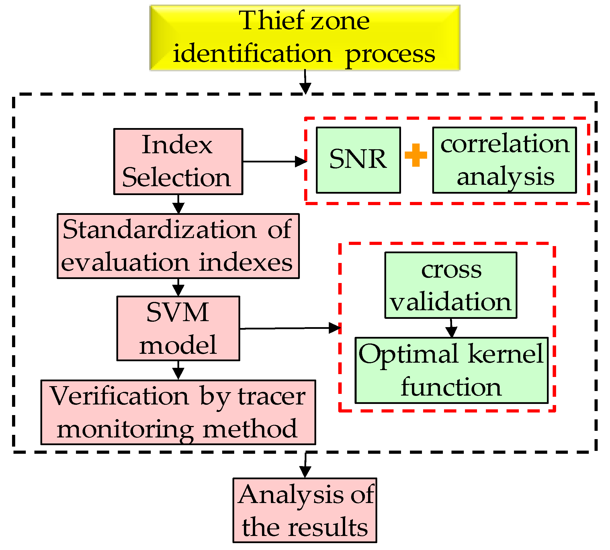
In this paper, the identification of the thief zone is mainly divided into the following four steps: First, the signal-to-noise ratio (SNR) and correlation analysis method are used to extract and select the thief zone evaluation indices. Second, the evaluation indices are standardized. Third, the cross-validation method is used to select the optimal kernel function, and the optimal kernel function is used to establish a support vector machine model. And finally, the identification results of the support vector machine (SVM) model are verified and analyzed by tracer monitoring method. The entire thief zone identification process is represented by a flow chart, as shown in
Figure 1.
2.1. Extraction and Selection of Thief Zone Evaluation Indices
In the process of extracting evaluation indices (such as permeability, porosity and water cut etc.), on the one hand, it is necessary to ensure that each index has a certain influence on the formation of the thief zone. On the other hand, it is also necessary to consider the actual data of oilfields to select indices that are easy to obtain data. The selection of an evaluation index refers to the process of selecting the most effective index combination for classification and recognition through screening the extracted indices or some transformation. The extraction and selection of evaluation indices are very important in the identification of thief zones, which directly determines the accuracy of the identification results.
In order to avoid the problem that the classification accuracy of SVM is too low due to too many indices and the correlation among indices, we comprehensively use signal-to-noise ratio and correlation analysis method to screen indices.
2.1.1. Signal-to-Noise Ratio
The signal-to-noise ratio (SNR) is used to rank the different attributes according to each index. The noise index can be effectively eliminated so that the index in front contains more classification information. Using these indices to classify can achieve higher accuracy. The amount of classification information contained in each index is determined by the following formula.
where
and
represent the mean value of the
ith feature of positive and negative samples respectively,
and
represent the standard deviation of the
ith feature of positive and negative samples respectively, and
SNRi represents the signal-to-noise ratio of the ith feature. The larger the
SNRi, the more classified information this feature contains, and the more favorable it is for classification. The advantages of SNR are its simple calculation process and less time-consuming nature. The disadvantage is that the interaction between the indicators is not taken into account.
2.1.2. Correlation Analysis
Correlation analysis is an important means of finding the relationship between indices. The correlation coefficient is a statistical index of the degree of a close relationship between response variables. The range of correlation coefficient is between 1 and −1. 1, which means that two variables are completely linearly correlated, −1 means that two variables are completely negatively correlated, and 0 means that two variables are not correlated. The closer the correlation coefficient is to 0, the weaker the correlation is. The following is the formula for calculating the correlation coefficient.
where
is the sample correlation coefficient,
is the sample covariance,
is the sample standard deviation of
X, and
is the sample standard deviation of
Y. The advantage of correlation analysis is that it can consider the interaction between indices.
2.2. Evaluation Index Standardization
In the multi-index evaluation system, due to the different nature of each evaluation index, there are usually different dimensions and quantities. When the level of each index is very different, if the original index value is used to analyze directly, the function of the higher value index in the comprehensive analysis will be highlighted, and the function of the lower value index will be relatively weakened. Therefore, in order to ensure the reliability of the results, it is necessary to standardize the original index data. At present, there are many methods of data standardization, which can be summed up as straight-line methods (such as the extreme value method or standard deviation method), broken line methods (such as the three-fold line method), and curve methods (such as semi-normal distribution). For simplicity and ease of calculation, this paper uses the “min–max standardization” method to standardize data.
where
x′ is normalized value,
x is sample value, max
A is the maximum value of attribute
A, min
A is the minimum value of attribute
A.
2.3. Support Vector Machine Model
As a classification method proposed by Vapnik et al., support vector machine [
35] is mainly applied in the field of pattern recognition and has many unique advantages in small-sample, nonlinear, and high-dimensional pattern recognition. In recent years, it has been successfully applied in image recognition [
36], signal processing [
37], gene map recognition [
38], and benign and malignant tumor recognition [
39], showing its advantages. Moreover, field data are characterized by extremely complex relationships and few records, which is suitable for classification prediction with support vector machines.
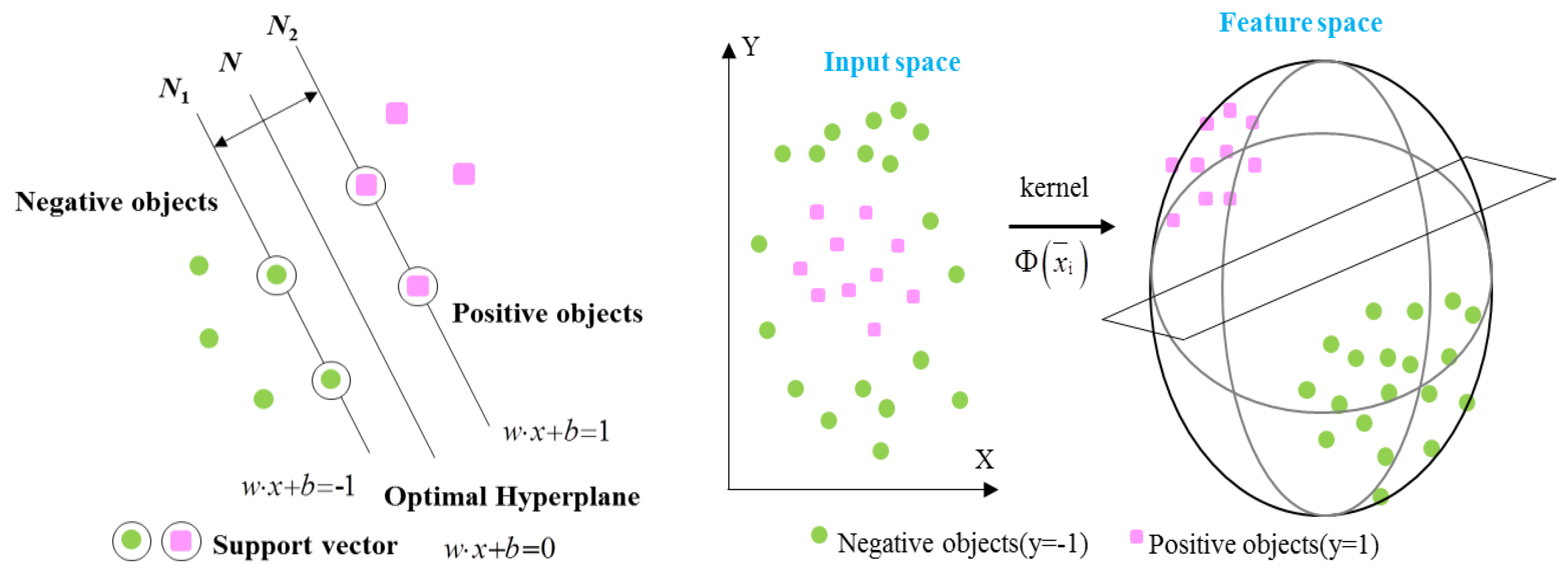
The basic principle of support vector machine is to map the sample space to a feature space of high or even infinite dimensions (namely Hilbert space) through nonlinear mapping, and to find the optimal classification surface in this feature space. Then, the nonlinear separable problem in the sample space can be transformed into a linear separable problem in the feature space by taking appropriate kernel functions.
For example, set the training sample set as
,
,
, where
l is the number of observed samples. If there is a hyperplane equation
to make the sample set satisfy
, the training set is called linearly separable.
Figure 2 shows the basic idea of SVM, in which the circular point and the square point represent two kinds of samples respectively. N is the classification hyperplane. N1 and N2 are the planes parallel to the classification hyperplane respectively. The samples on them are closest to the classification hyperplane, and the distance between them is the classification interval. The so-called optimal classification hyperplane requires that the classification plane not only correctly separates the two categories, but also maximizes the classification interval, which is
. The nearest vector to the optimal hyperplane is the support vector, and the distance between the support vector and the hyperplane is
. Thus, the problem of constructing the optimal hyperplane is transformed into the problem of seeking the optimal solution of quadratic programming.
The objective function is:
The optimal classification function obtained after solving the above problems is
When the training sample is linearly indivisible, slack variables
need to be introduced. Then, SVM can be expressed as the following quadratic optimization problem, where
C > 0 is the penalty parameter.
To solve this quadratic optimization problem, the kernel function
k(
xi,
yi) needs to be introduced, and the expression of SVM can be obtained as follows:
For the nonlinear problem, the input space needs to be mapped to a high-dimensional feature space by the kernel function
k(
xi,
yi), as shown in
Figure 2. Because the dual problem above only involves the inner product operation between training samples, as long as the inner product of the kernel function
k(
xi,
yi) is equal to the inner product of X and Y mapped in the high-dimensional feature space, a support vector machine can be determined by the kernel function
k(
xi,
yi), so as to avoid the dimension disaster problem in the feature space.
In general, the four kernel functions include the following:
- (1)
The linear kernel function K(x, y) = x·y;
- (2)
The binomial kernel function K(x, y) = [(x·y) + 1]d;
- (3)
The radial basis kernel function (RBF) K(x, y) = exp(−|x − y|2/d2); and
- (4)
The sigmoid kernel function (neural network) K(x, y) = tanh(a(x·y) + b).
Each of the four functions has its own characteristics, as shown in
Table 1 below.
In order to select the optimal kernel function, we adopted a five times cross validation method (that is, the sample database data set is randomly divided into five parts, each part is taken as a test set in turn, and the rest is taken as a training set) for training and testing.
Sen,
Spe, and
Q were used for statistical analysis:
where the positive samples are non-thief zone well groups known in the oilfield. Negative samples are thief zone well groups known in the oilfield. True positive
TP indicates the number of samples accurately judged as positive samples in the test set. False negative
FN indicates the number of samples wrongly judged as negative in the test set. True negative
TN indicates the number of samples accurately judged as negative samples in the test set, and false positive
FP indicates the number of samples wrongly judged as positive in the test set.
Sen is the sensitivity of positive samples in the test set, and
Spe is the specificity of negative samples in the test set. The larger the
Sen, the stronger the recognition ability of the positive sample. The larger the
Spe, the better the discrimination effect on negative samples.
Q is the total test accuracy.
Finally, the kernel function with the highest total test accuracy and the strongest sensitivity to negative samples (i.e., the thief zone) that satisfies the applicable situation should be selected as the optimal kernel function. Then, the selected thief zone evaluation indices are taken as the input, and the corresponding thief zone recognition results are taken as the output. By using the optimized kernel function and through continuous training and learning, the trained SVM model can be used as a thief zone recognition model.
3. Examples of Application
Taking a block of M oil field as an example, based on the existing data of the oil field, the thief zone identification was carried out according to the above method, and the identification results were verified by tracer monitoring method.
3.1. Oilfield Overview
M oilfield is a heterogeneous sandstone reservoir with positive rhythm deposition, with a development area of 9.56 km2 and geological reserves of 1556.51 × 104 t. The top burial depth of the oil layer is from 751 to 1047 m, and the oil–water interface depth is from 1088 to 1197 m. The reservoir’s original formation pressure was 11.07 Mpa. The average air permeability of this block in M oilfield is 632 × 10−3 μm2, porosity is 27.4%, effective thickness is 43.5 m, reservoir temperature is 42.7~51 °C, and underground crude oil density is 0.89 g/cm3.
After more than 20 years of water flooding development, the comprehensive water cut of M oilfield has reached 82%. Long-term water flooding development leads to serious development of thief zones in this oilfield, and a large amount of injected water rushes along the thief zones, resulting in inefficient or even invalid circulation of injected water in many blocks, which greatly reduces the oilfield development effect and economic benefits. Therefore, strengthening the identification of thief zones has become a prominent task.
3.2. Evaluation Indices
According to the extraction principles of the above evaluation indices and considering the geological factors and development factors that affect the formation of thief zones, the indices, such as permeability K, porosity , effective thickness h, cumulative water injection Wi, daily water injection qi, water injection pressure Pwo, bottom hole pressure Pwf, water cut fw, cumulative liquid production Wl, and daily liquid production ql were selected.
By calculating the signal-to-noise ratio (SNR) and correlation coefficient, the contribution of each index to classification, and the correlation among the indices were obtained simultaneously, as shown in
Table 2 and
Table 3.
Numbers 1–10 in
Table 2 indicate the contribution degree of each index to classification: 1 indicates the largest contribution degree, and 10 indicates the smallest contribution degree, which decreases in turn. In
Table 2, it can be seen that the SNR of water injection pressure was 0.03, which contributed little to the classification, followed by daily liquid production and bottom hole pressure. The maximum contribution of daily water injection to classification was 0.32. Considering the result of the SNR calculation, the main objects of screening were water injection pressure, daily liquid production, and bottom hole pressure.
Numbers 1–5 in
Table 3 indicate the degree of correlation among the indices: 1 indicates the strongest degree of correlation, and 5 indicates the weakest degree of correlation, which decreases in turn. The indices listed in the table are those whose correlation coefficient is greater than 0.5. Those whose correlation coefficient is less than 0.5 have a weak correlation and were not considered for the time being. In
Table 3, we can clearly see the correlation among the indices. Considering the results of correlation calculation, daily water injection, daily liquid production, effective thickness, porosity, and cumulative water injection were the main targets for screening.
According to
Table 2 and
Table 3, from the perspective of oilfield development, the permeability, porosity, and effective thickness are the basic indices of the oilfield, and the greater the permeability, porosity, and effective thickness, the more obvious the heterogeneity of the reservoir, and the easier it is to form the thief zone. Therefore, these indices should be retained. Because daily water injection and daily liquid production, cumulative water injection and cumulative liquid production, and water injection pressure and bottom hole pressure are three pairs of one-to-one corresponding indices, and daily water injection also had a great impact on the cumulative water injection and water injection pressure, in the screening process, only one pair of indices with the largest contribution could be retained. The SNR of daily water injection was the highest, and its contribution to classification was the highest. However, it also had a high correlation with other indices, which may lead to low classification accuracy. In addition, the SNR of daily liquid production was 0.06, which means it makes a low contribution to classification. Therefore, the pair of indices of daily water injection and daily liquid production was ignored. In addition, because the SNRs of water injection pressure and bottom hole pressure were relatively low, they did not contribute much to classification. Therefore, the pair of indices of water injection pressure and bottom hole pressure was also ignored. Thus, the indices of cumulative water injection and cumulative liquid production were retained.
In summary, the optimal evaluation index system is shown in
Table 4.
3.3. SVM Identification Method
According to the actual working conditions of M oilfield, after years of verification by field experts and actual statistical data of the oil field, 20 groups of typical well groups with highly developed thief zones and 20 groups of ordinary well groups with good production conditions were obtained. The 40 groups of well groups were taken as the training samples for discrimination. The sample database of production data after statistical standardization is shown in
Table 5.
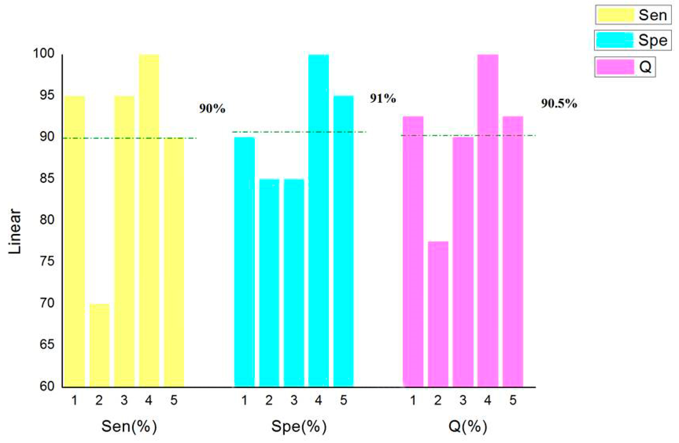
In order to select the kernel function with the best recognition effect, five cross-validations were carried out to calculate
Sen,
Spe, and
Q. The results are shown in
Figure 3.
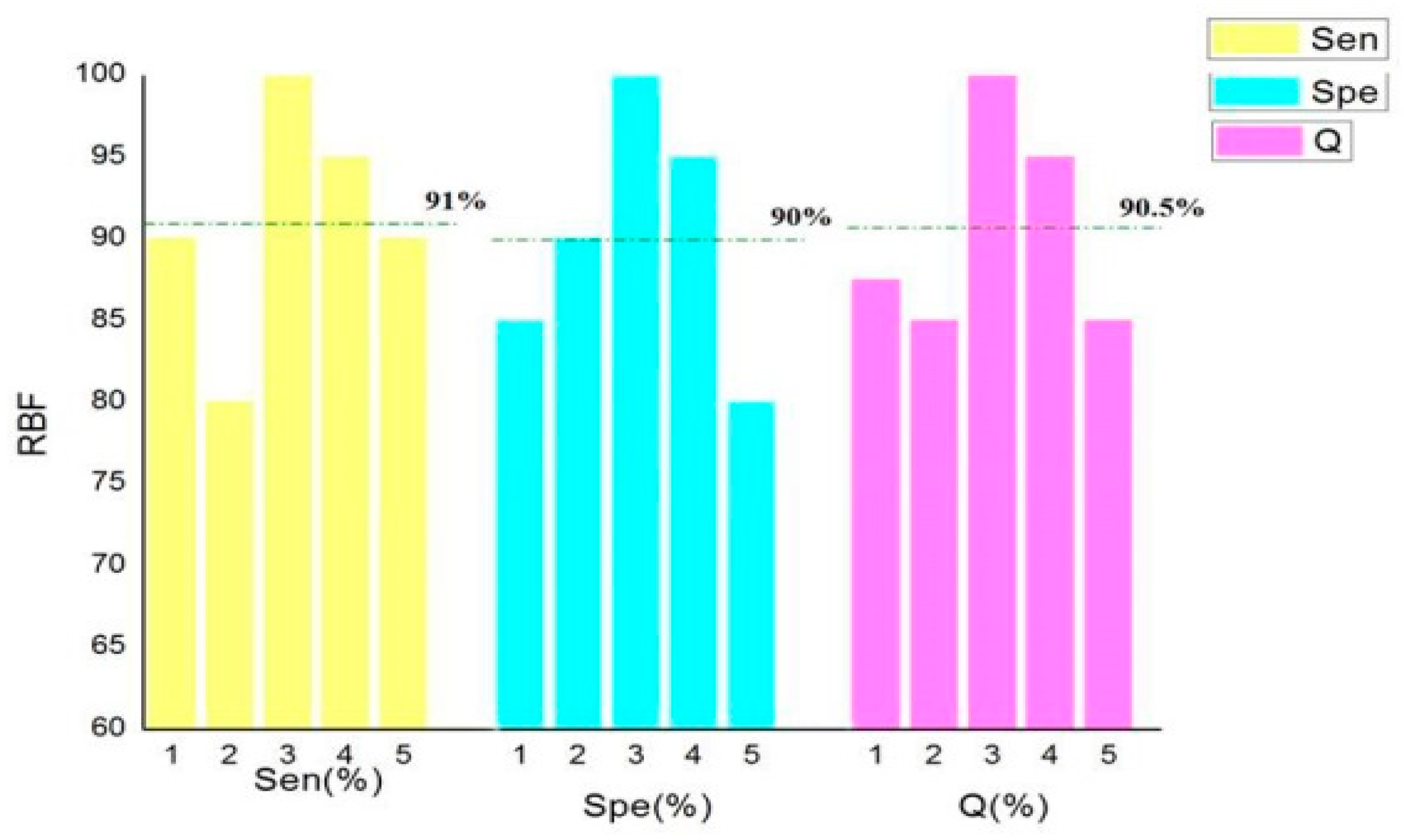
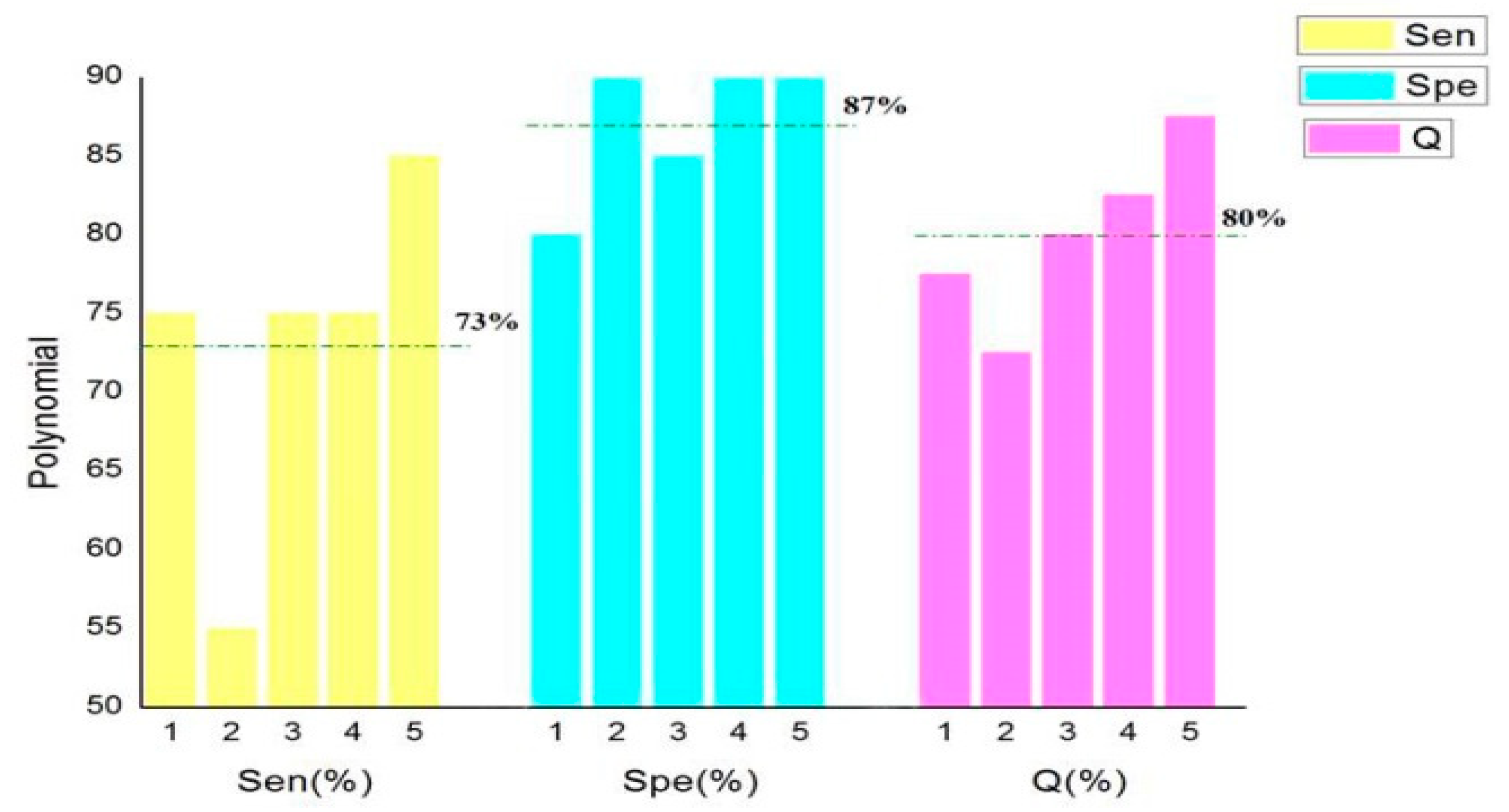
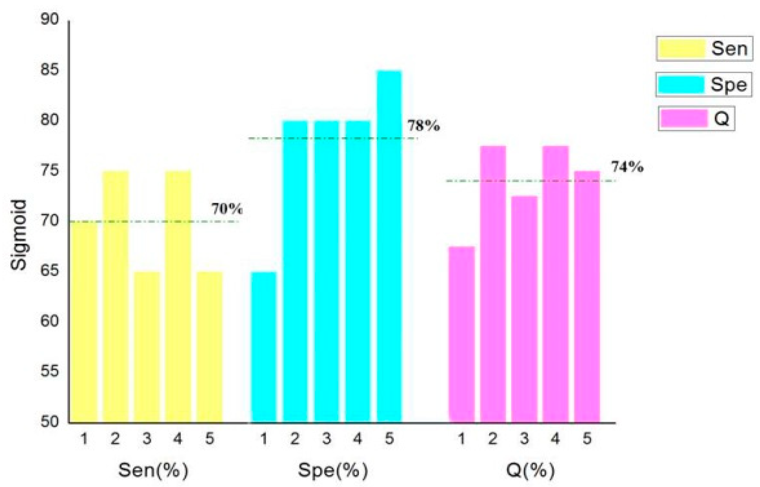
It can be seen in
Figure 3,
Figure 4,
Figure 5 and
Figure 6 that the classification accuracy of linear kernel function and radial basis kernel function was 90.5%, the polynomial kernel function was 80%, and the Sigmoid kernel function was 74% when the above four kernel functions were classified by the cross-validation method. In the classification using linear kernel function, the sensitivity of the positive sample was 90% and that of the negative sample was 91%. In the classification using radial basis kernel function, the sensitivity of the positive samples was 91%, and that of the negative samples was 90%. The purpose of this paper was to identify the thief zone, that is, to identify the negative sample. Therefore, the linear kernel function with the highest accuracy and the highest negative sample sensitivity were ultimately selected. Although many studies have reported that, in most cases, the radial basis kernel function has the strongest classification ability, it can be seen from the figure above that the linear kernel function has the highest accuracy and the strongest recognition ability with respect to the negative samples. This shows the necessity of the optimized kernel function and improves the reliability and stability of the model.
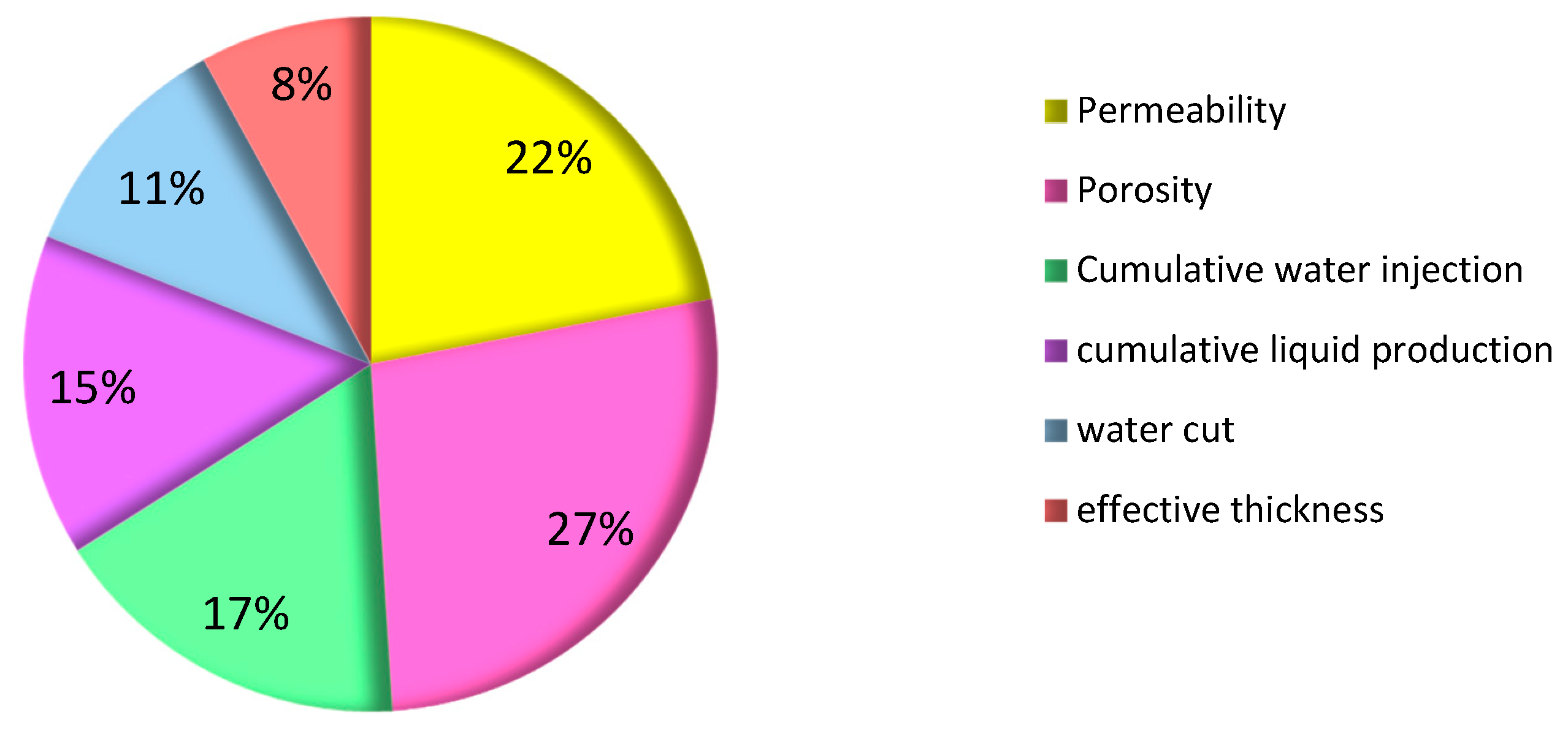
The importance of each index of the thief zone identification model obtained by using the optimized kernel function (the linear kernel function) and the sample database to the classification is shown in
Figure 7.
It can be seen in
Figure 7 that porosity had the largest impact on classification, with a weight of 27%. This was because, after a long period of water flooding in M oilfield, the radius of the local pore throat in the reservoir increased, the degree of cementation weakened, and the porosity increased. Moreover, the oilfield has entered the later stage of development, and the water flooding development has failed to achieve the ideal oil-displacement effect. Therefore, a large amount of injected water rushed along the thief zone, resulting in an inefficient or even invalid circulation of injected water in many blocks. Porosity has become an important index affecting the formation of the thief zone. The second most important index was permeability, with a weight of 22%. This is because the greater the permeability, the smaller the vertical migration resistance of the water in the formation during water flooding development, causing the water to gradually converge at the bottom of the permeable layer along the formation direction, which forms the thief zone. The next most important indices were cumulative water injection, cumulative liquid production, and water cut, with weights of 17%, 15%, and 11%, respectively. Cumulative water injection, cumulative liquid production, and water cut were the dynamic response indices of the thief zone. Based on the comprehensive analysis of the cumulative water injection and the cumulative liquid production, when the cumulative water injection is constant, the larger the cumulative liquid production, the better the connectivity between the production well and the water injection well, and the greater the possibility of forming the thief zone. The value of water cut reflects the amount of water in the produced fluid and the amount of water injected into the production well. The higher the water cut, the better the connectivity between the production well and the injection well, and the easier it is to form the thief zone.
The above model was applied to identify the thief zone of 82 groups of wells injected with tracer in M oilfield. There were four kinds of tracers used in the identification, namely NH
4SCN, I
135, NH
4NO
3, and C
28H
20N
3O
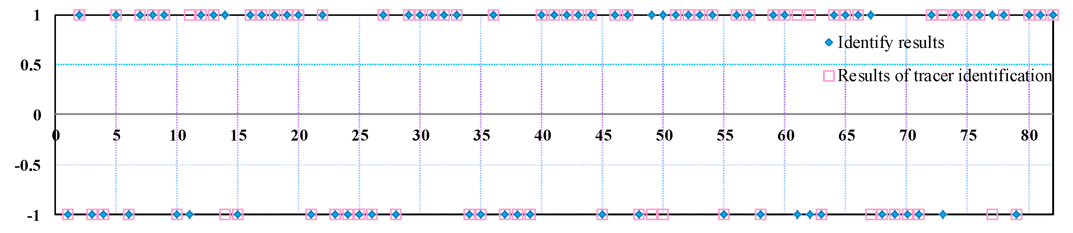
5. The earliest tracer injection occurred on 3 May 2014, and the latest occurred on 16 September 2016. The first tracer ended on 4 July 2016, and the last ended on 19 December 2017. The average breakthrough time of tracer was 6.4 months. The fastest breakthrough time was 2.1 months, and the slowest was 7.8 months. The identification result of the well group in which the tracer was detected was −1, while that of the group without the tracer detected was 1. The identification results and tracer identification results are shown in
Figure 8. When the blue dot is inside the red square, then the algorithm correctly identified a thief zone, when it is not, it means wrong recognition.
As can be seen in
Figure 8, 27 groups of thief zone wells and 46 groups of non-thief zone wells were identified by the two methods. Additionally, 32 groups of thief zone wells and 50 groups of non-thief zone wells were identified by tracer. Thus, the recognition accuracy of the negative samples was 84.375%, that of the positive samples was 92%, and the total accuracy was 89.02%. It has been proven, therefore, that the method has a high total recognition accuracy and can provide certain reference value for the formulation of profile control and water plugging schemes in the high water cut period of an oil reservoir.
4. Conclusions
In this paper, a support vector machine was used to identify thief zones in a mature oil reservoir. The principle and identification flow of the method were introduced. Then, the method was applied to 82 groups of wells in M oilfield and verified by the tracer monitoring method.
(1) Through the analysis of the SVM identification results and tracer identification results, it was found that the thief zone of M oilfield is seriously developed, and 33% of the 82 well groups identified by the two methods were identified as thief zones. This situation should be paid attention to and corresponding profile control and water shutoff measures should be taken to improve the thief zone.
(2) Through the analysis of the index weight affecting the thief zone, it was found that porosity has the largest influence on the formation of the thief zone, followed by permeability and then cumulative water injection, cumulative liquid production, and water cut.
(3) By using signal-to-noise ratio and correlation analysis methods to screen the indices, it was found that our proposed method can effectively avoid the problem of the classification accuracy of SVM being too low due to too many indices and the correlation between various indices.
(4) By comparing the SVM method with other reservoir engineering methods to identify the thief zone, it was found that the SVM method can effectively avoid the influence of human factors on the identification results, and the identification results were more objective and accurate.
(5) The identification results were verified by the tracer monitoring method, and it was found that the total accuracy of the SVM method in identifying the thief zone was 89.02%, that of the positive sample was 92%, and that of the negative sample was 84.375%.


