Prediction of CO2 Solubility in Ionic Liquids Based on Multi-Model Fusion Method


Abstract
:1. Introduction
2. Methods
2.1. Single Modeling Method
2.1.1. Back Propagation Neural Networks
2.1.2. Support Vector Machine
2.1.3. Extreme Learning Machine
2.2. Linear Fusion Method
2.2.1. Minimum Squared Error
2.2.2. Information Entropy
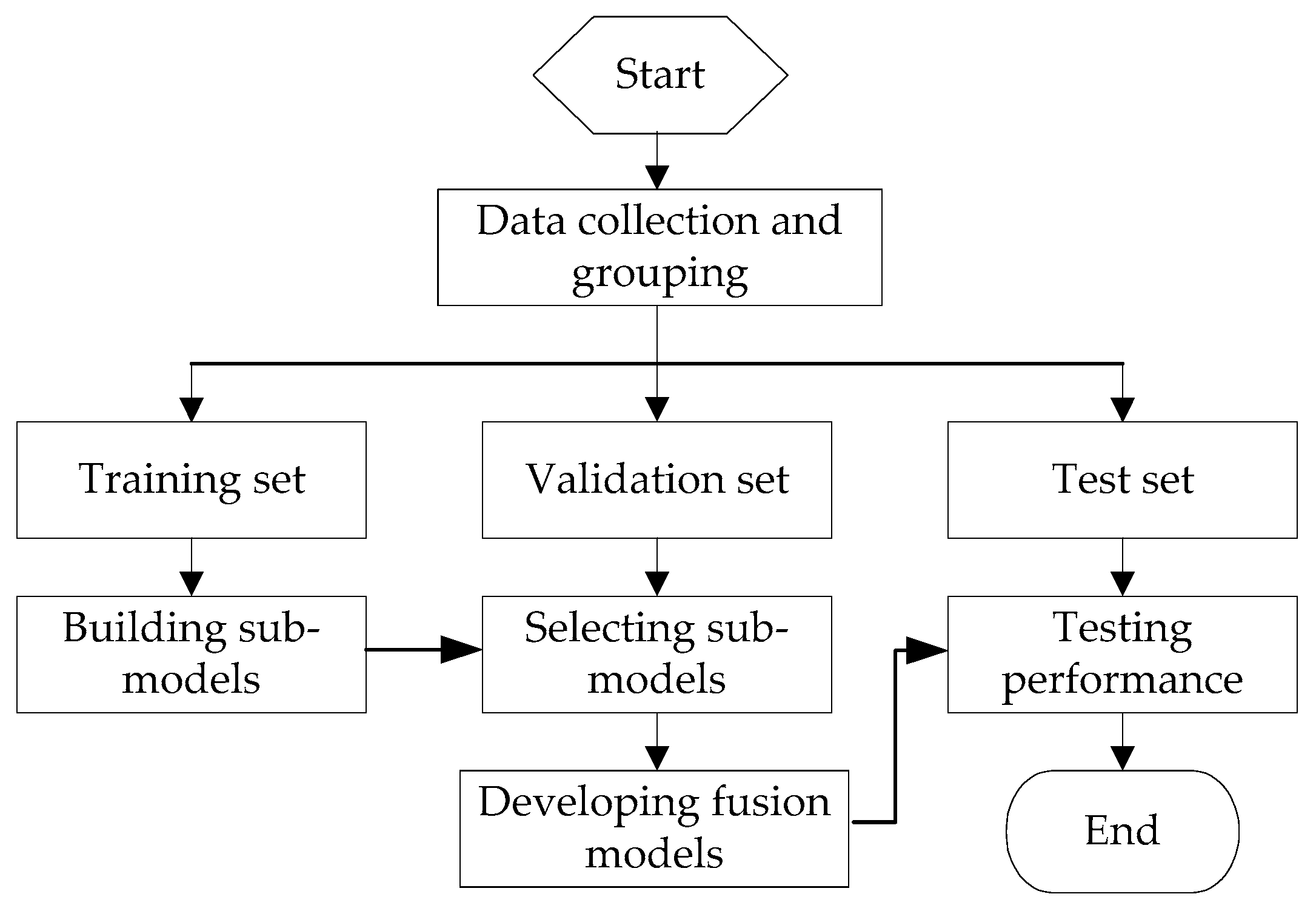
2.3. Implementation Steps
3. Results and Discussion
3.1. Data Collecting and Grouping
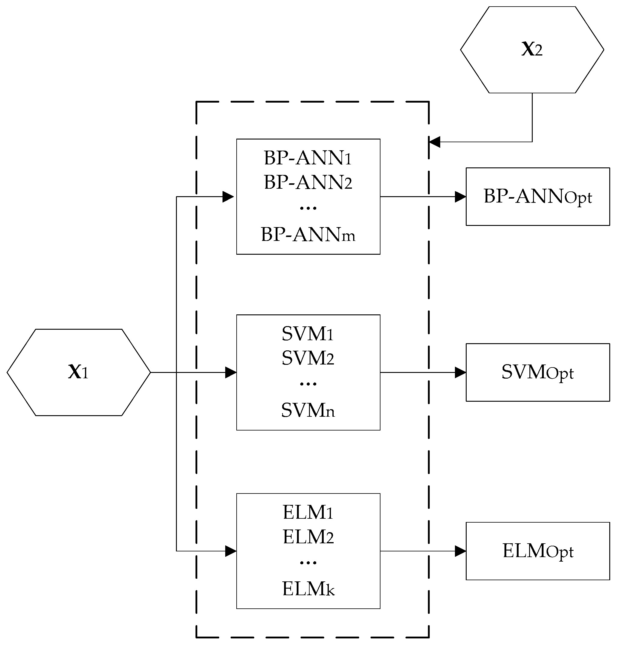
3.2. Fusion Model Development
3.2.1. Sub-Models Development
3.2.2. Sub-Models Evaluation
3.2.3. Sub-Models Fusion
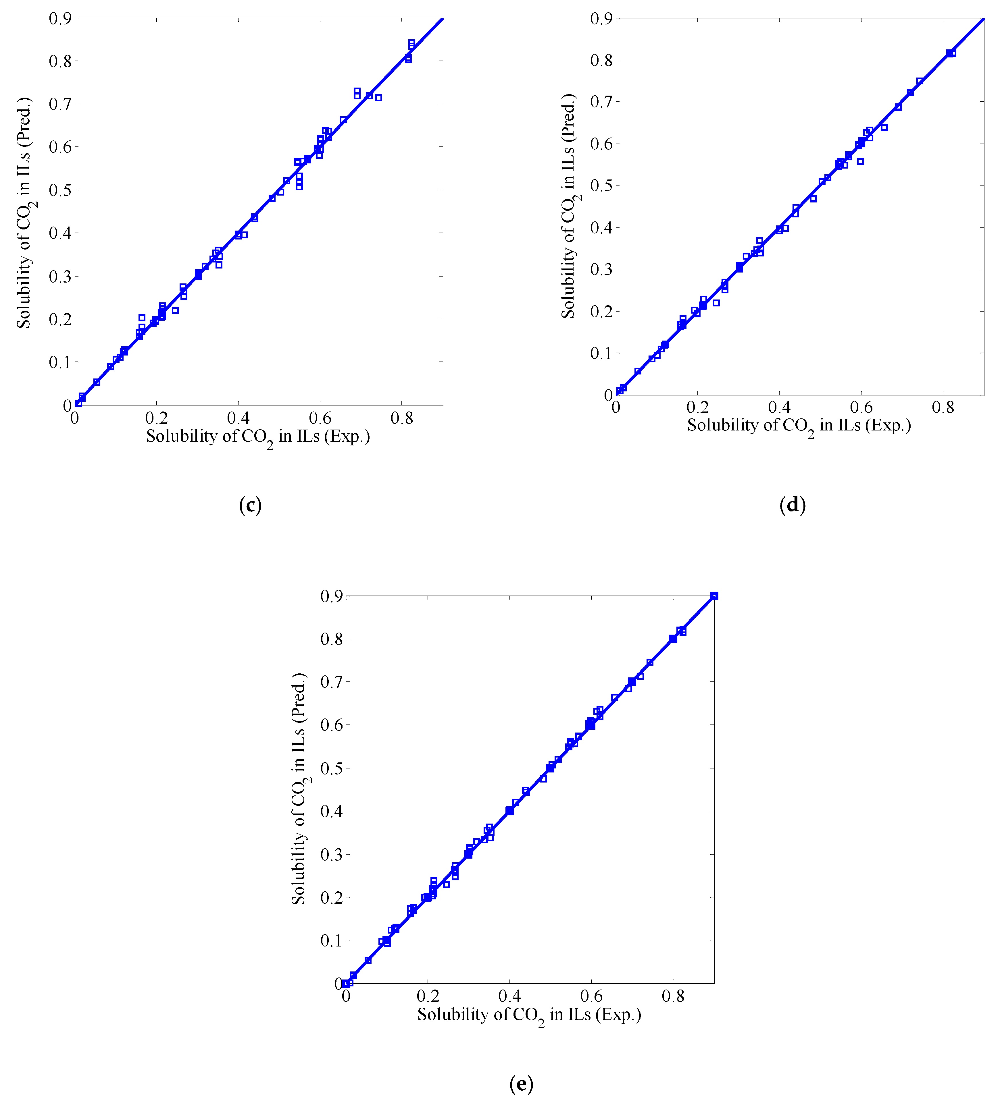
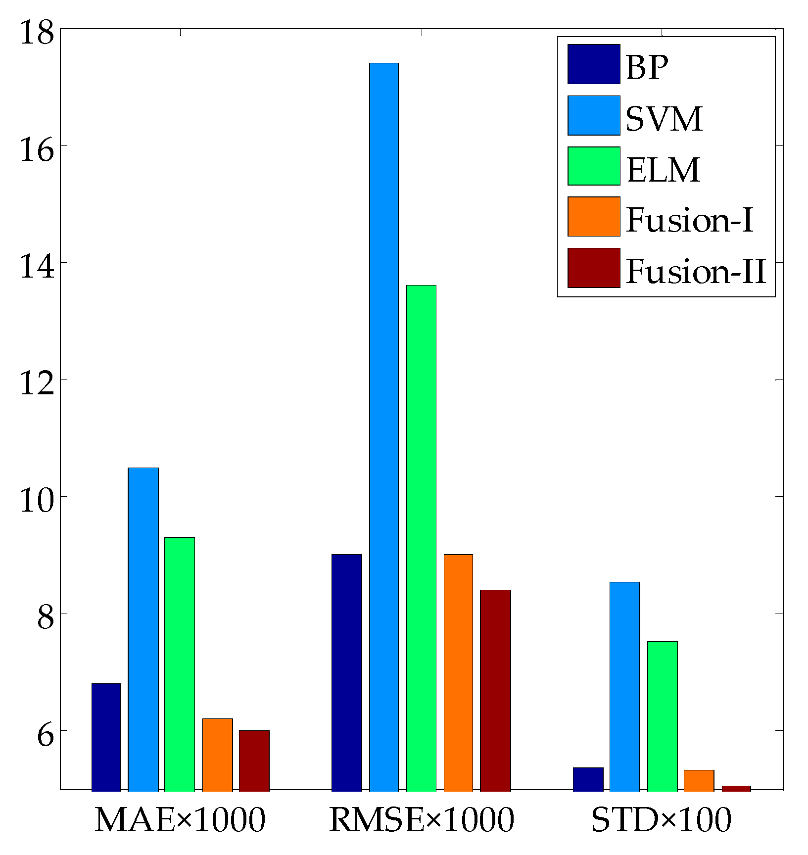
3.3. Fusion Model Testing
4. Conclusions
Author Contributions
Funding
Acknowledgments
Conflicts of Interest
References
- Zhao, Z.J.; Dong, H.F.; Zhang, X.P. The research progress of CO2 capture with ionic liquids. Chin. J. Chem. Eng. 2012, 20, 120–129. [Google Scholar] [CrossRef]
- Zhang, S.J.; Liu, X.M.; Yao, X.Q.; Dong, H.F.; Zhang, X.P. Frontiers, progresses and applications of ionic liquids. Sci. China 2009, 39, 1134–1144. [Google Scholar]
- Bara, J.E.; Gin, D.L.; Noble, R.D. Effect of anion on gas separation performance of polymer-room-temperature ionic liquid composite membranes. Ind. Eng. Chem. Res. 2008, 47, 9919–9924. [Google Scholar] [CrossRef]
- Abejón, R.; Rabadán, J.; Lanza, S.; Abejón, A.; Garea, A.; Irabien, A. Supported ionic liquid membranes for separation of lignin aqueous solutions. Processes 2018, 6, 143. [Google Scholar] [CrossRef]
- Brennecke, J.F.; Gurkan, B.E. Ionic liquids for CO2 capture and emission reduction. J. Phys. Chem. Lett. 2017, 1, 3459–3464. [Google Scholar] [CrossRef]
- Gurkan, B.; Goodrich, B.F.; Mindrup, E.M.; Ficke, L.E.; Masse, M.; Seo, S.; Senftle, T.P.; Wu, H.; Glaser, M.F.; Shah, J.K.; et al. Molecular design of high capacity, low viscosity, chemically tunable ionic liquids for CO2 capture. J. Phys. Chem. Lett. 2017, 1, 3494–3499. [Google Scholar] [CrossRef]
- Bahmani, A.R.; Sabzi, F.; Bahmani, M. Prediction of solubility of sulfur dioxide in ionic liquids using artificial neural network. J. Mol. Liq. 2015, 211, 395–400. [Google Scholar] [CrossRef]
- Ding, J.; Xiong, Y.; Yu, D.H. Solubility of CO2 in ionic liquids—measuring and modeling methods. Chem. Ind. Eng. Prog. 2012, 31, 732–741. [Google Scholar]
- Jaubert, J.N.; Vitu, S.; Mutelet, F. Extension of the PPR78 model (predictive 1978, Peng-Robinson EOS with temperature dependent kij calculated through a group contribution method) to systems containing aromatic compounds. Fluid Phase Equilibr. 2006, 237, 193–211. [Google Scholar] [CrossRef]
- Lei, Z.G.; Dai, C.N.; Chen, B.H. Gas solubility in ionic liquids. Chem. Rev. 2014, 114, 1289–1326. [Google Scholar] [CrossRef]
- Soave, G. Equilibrium constants from a modified Redlich-Kwong equation of state. Chem. Eng. Sci. 1972, 27, 1197–1203. [Google Scholar] [CrossRef]
- Breure, B.; Bottini, S.B.; Witkamp, G.J.; Peters, C.J. Thermodynamic modeling of the phase behavior of binary systems of ionic liquids and carbon dioxide with the group contribution equation of state. J. Phys. Chem. B 2007, 111, 14265–14270. [Google Scholar] [CrossRef]
- Carvalho, P.J.; Álvarez, V.H.; Marrucho, I.M.; Aznar, M.; Coutinho, J.P. High pressure phase behavior of carbon dioxide in 1-butyl-3-methylimidazolium bis(trifluoromethylsulfonyl)imide and 1-butyl-3-methylimidazolium dicyanamide ionic liquids. J. Supercrit. Fluid. 2009, 50, 105–111. [Google Scholar] [CrossRef]
- Bavoh, C.B.; Lal, B.; Nashed, O.; Khan, M.S.; Keong, L.K.; Bustam, M.A. COSMO-RS: An ionic liquid prescreening tool for gas hydrate mitigation. Chin. J. Chem. Eng. 2016, 24, 1619–1624. [Google Scholar] [CrossRef]
- Gholizadeh, A.; Sabzi, F. Prediction of CO2 sorption in poly(ionic liquid)s using ANN-GC and ANFIS-GC models. Int. J. Greenh. Gas Con. 2017, 63, 95–106. [Google Scholar] [CrossRef]
- Ghiasi, M.M.; Mohammadi, A.H. Application of decision tree learning in modelling CO2 equilibrium absorption in ionic liquids. J. Mol. Liq. 2017, 242, 594–605. [Google Scholar] [CrossRef]
- Eslamimanesh, A.; Gharagheizi, F.; Mohammadi, A.H.; Richon, D. Artificial Neural Network modeling of solubility of supercritical carbon dioxide in 24 commonly used ionic liquids. Chem. Eng. Sci. 2011, 66, 3039–3044. [Google Scholar] [CrossRef]
- Lashkarbolooki, M.; Shafipour, Z.S.; Hezave, A.Z.; Farmani, H. Use of artificial neural networks for prediction of phase equilibria in the binary system containing carbon dioxide. J. Supercrit. Fluid. 2013, 75, 144–151. [Google Scholar] [CrossRef]
- Lashkarbolooki, M.; Shafipour, Z.S.; Hezave, A.Z. Trainable cascade-forward back-propagation network modeling of spearmint oil extraction in a packed bed using SC-CO2. J. Supercrit. Fluid. 2013, 73, 108–115. [Google Scholar] [CrossRef]
- Tatar, A.; Naseri, S.; Bahadori, M.; Hezave, A.Z.; Kashiwao, T.; Bahadori, A.; Darvish, H. Prediction of carbon dioxide solubility in ionic liquids using MLP and radial basis function (RBF) neural networks. J. Taiwan Inst. Chem. E. 2016, 60, 151–164. [Google Scholar] [CrossRef]
- Yang, Y.; Chen, Y.H.; Wang, Y.C.; Li, C.H.; Li, L. Modelling a combined method based on ANFIS and neural network improved by DE algorithm: A case study for short-term electricity demand forecasting. Appl. Soft Comput. 2016, 49, 663–675. [Google Scholar] [CrossRef]
- Zuan, P.; Huang, Y. Prediction of sliding slope displacement based on intelligent algorithm. Wirel. Pers. Commun. 2018, 102, 3141–3157. [Google Scholar] [CrossRef]
- Xu, Q.; Chen, J.Y.; Liu, X.P.; Li, J.; Yuan, C.Y. An ABC-BP-ANN algorithm for semi-active control for magnetorheological damper. KSCE J. Civ. Eng. 2017, 21, 2310–2321. [Google Scholar] [CrossRef]
- Sridhar, D.V.; Bartlett, E.B.; Seagrave, R.C. Information theoretic subset selection for neural network models. Comput. Chem. Eng. 1998, 22, 613–626. [Google Scholar] [CrossRef]
- Tatar, A.; Yassin, M.R.; Rezaee, M.; Aghajafari, A.H.; Shokrollahi, H. Applying a robust solution based on expert systems and GA evolutionary algorithm for prognosticating residual gas saturation in water drive gas reservoirs. J. Nat. Gas Sci. Eng. 2014, 21, 79–94. [Google Scholar] [CrossRef]
- Ling, H.; Qian, C.; Kang, W.; Liang, C.; Chen, H. Combination of Support Vector Machine and K-Fold cross validation to predict compressive strength of concrete in marine environment. Constr. Build. Mater. 2019, 206, 355–363. [Google Scholar] [CrossRef]
- Zhou, T.; Lu, H.; Wang, W.W.; Yong, X. GA-SVM based feature selection and parameter optimization in hospitalization expense modeling. Appl. Soft Comput. 2019, 75, 323–332. [Google Scholar]
- Huang, G.B.; Zhu, Q.Y.; Siew, C.K. Extreme learning machine: Theory and applications. Neurocomputing 2006, 70, 489–501. [Google Scholar] [CrossRef]
- Lan, Y.; Soh, Y.C.; Huang, G.B. Ensemble of online sequential extreme learning machine. Neurocomputing 2009, 72, 3391–3395. [Google Scholar] [CrossRef]
- Huang, G.B.; Ding, X.J.; Zhou, H.M. Optimization method based extreme learning machine for classification. Neurocomputing 2010, 74, 155–163. [Google Scholar] [CrossRef]
- Wang, S.H.; Li, H.F.; Zhang, Y.J.; Zou, Z.S. A hybrid ensemble model based on ELM and improved AdaBoost.RT algorithm for predicting the iron ore sintering characters. Comput. Intel. Neurosc. 2019, 60, 1–11. [Google Scholar] [CrossRef] [PubMed]
- Kurnaz, T.F.; Kaya, Y. The comparison of the performance of ELM, BRNN, and SVM methods for the prediction of compression index of clays. Arab. J. Geosci. 2018, 11, 1–14. [Google Scholar]
- Shannon, C.E. A mathematical theory of communication. Bell Labs Tech. J. 1948, 27, 379–423. [Google Scholar] [CrossRef]
- Baghban, A.; Ahmadi, M.A.; Shahraki, B.H. Prediction carbon dioxide solubility in presence of various ionic liquids using computational intelligence approaches. J. Supercrit. Fluid. 2015, 98, 50–64. [Google Scholar] [CrossRef]
- Sedghamiz, M.A.; Rasoolzadeh, A.; Rahimpour, M.R. The ability of artificial neural network in prediction of the acid gases solubility in different ionic liquids. J. CO2 Util. 2015, 9, 39–47. [Google Scholar] [CrossRef]
- Haghbakhsh, R.; Soleymani, H.; Raeissi, S. A simple correlation to predict high pressure solubility of carbon dioxide in 27 commonly used ionic liquids. J. Supercrit. Fluid. 2013, 77, 158–166. [Google Scholar] [CrossRef]
- Schilderman, A.M.; Raeissi, S.; Peters, C.J. Solubility of carbon dioxide in the ionic liquid 1-ethyl-3-methylimidazolium bis(trifluoromethylsulfonyl)imide. Fluid Phase Equilibr. 2007, 260, 19–22. [Google Scholar] [CrossRef]
- Jalili, A.H.; Mehdizadeh, A.; Shokouhi, M.; Ahmadi, A.N.; Fateminassab, F. Solubility and diffusion of CO2 and H2S in the ionic liquid 1-ethyl-3-methylimidazolium ethylsulfate. J. Chem. Thermodyn. 2010, 42, 1298–1303. [Google Scholar] [CrossRef]
- Lashkarbolooki, M.; Vaferi, B.; Rahimpour, M.R. Comparison the capability of artificial neural network (ANN) and EOS for prediction of solid solubilities in supercritical carbon dioxide. Fluid Phase Equilibr. 2011, 308, 35–43. [Google Scholar] [CrossRef]
- Tagiuri, A.; Sumon, K.Z.; Henni, A. Solubility of carbon dioxide in three [Tf2N] ionic liquids. Fluid Phase Equilibr. 2014, 380, 39–47. [Google Scholar] [CrossRef]
- Cybenko, G. Approximation by superpositions of a sigmoidal function. Math. Control Signal. 1992, 5, 455. [Google Scholar] [CrossRef]


| No. | Ionic Liquids | MW (g/mol) | Tc (k) | Pc (MPa) | Acentric Factor (w) |
|---|---|---|---|---|---|
| 1 | [BMIM][BF4] | 226.03 | 623.3 | 2.04 | 0.8489 |
| 2 | [EMIM][TF2N] | 391.30 | 788.05 | 3.31 | 1.225 |
| 3 | [EMIM][ETSO4] | 236.29 | 1061.1 | 4.04 | 0.3368 |
| 4 | [HMIM][TF2N] | 447.92 | 1292.78 | 2.3888 | 0.3893 |
| 5 | [HMIM][TFO] | 316.34 | 1055.6 | 2.4954 | 0.489 |
| 6 | [HMIM][BF4] | 254.08 | 716.61 | 1.7941 | 0.6589 |
| 7 | [HMIM][MESO4] | 278.37 | 1110.84 | 2.9611 | 0.4899 |
| 8 | [BMMIM][TF2N] | 433.4 | 1255.8 | 2.031 | 0.3193 |
| 9 | [HMIM][PF6] | 312.24 | 759.16 | 1.5499 | 0.9385 |
| No. | Ionic Liquids | Temperature Range (K) | Pressure Range (MPa) | CO2 Solubility Range (Mole Fraction) | No. of Samples | Refs. |
|---|---|---|---|---|---|---|
| 1 | [BMIM][BF4] | 278.47–368.22 | 0.587–67.620 | 0.102–0.602 | 104 | [35,36] |
| 2 | [EMIM][TF2N] | 312.10–410.90 | 0.626–14.329 | 0.123–0.593 | 77 | [35,37] |
| 3 | [EMIM][ETSO4] | 303.15–353.15 | 0.122–1.546 | 0.008–0.132 | 39 | [35,38] |
| 4 | [HMIM][TF2N] | 303.15–373.15 | 0.420–45.280 | 0.165–0.824 | 64 | [20,39] |
| 5 | [HMIM][TFO] | 303.15–373.15 | 1.420–100.120 | 0.267–0.816 | 64 | [20,39] |
| 6 | [HMIM][BF4] | 303.15–373.15 | 1.200–41.690 | 0.212–0.622 | 48 | [20,39] |
| 7 | [HMIM][MESO4] | 303.15–373.15 | 0.870–50.140 | 0.158–0.602 | 48 | [20,39] |
| 8 | [BMMIM][TF2N] | 298.15–343.15 | 0.010–1.900 | 0.002–0.211 | 36 | [20,40] |
| 9 | [HMIM][PF6] | 243.15–373.15 | 0.220–55.630 | 0.216–0.691 | 64 | [20,39] |
| No. of Hidden Layer Neurons | MAE | RMSE | R2 | STD |
|---|---|---|---|---|
| 3 | 0.0081 | 0.0114 | 0.9973 | 0.0659 |
| 4 | 0.0062 | 0.0085 | 0.9985 | 0.0499 |
| 5 | 0.0076 | 0.0099 | 0.9979 | 0.0616 |
| 6 | 0.0064 | 0.0088 | 0.9983 | 0.0521 |
| 7 | 0.0063 | 0.0090 | 0.9983 | 0.0512 |
| 8 | 0.0082 | 0.0108 | 0.9975 | 0.0661 |
| 9 | 0.0064 | 0.0092 | 0.9982 | 0.0521 |
| 10 | 0.0070 | 0.0096 | 0.9981 | 0.0567 |
| Type of Kernel Function | MAE | RMSE | R2 | STD |
|---|---|---|---|---|
| Polynomial kernel function | 0.0135 | 0.0196 | 0.9922 | 0.1091 |
| Radial basis kernel function | 0.0122 | 0.0180 | 0.9928 | 0.0992 |
| Sigmoid kernel function | 0.0269 | 0.0363 | 0.9727 | 0.2180 |
| No. of Neurons | Type of Activation Function | MAE | RMSE | R2 | STD |
|---|---|---|---|---|---|
| 148 | sigmoid | 0.0124 | 0.0176 | 0.9970 | 0.1007 |
| 149 | sigmoid | 0.0106 | 0.0149 | 0.9938 | 0.0856 |
| 150 | sigmoid | 0.0113 | 0.0158 | 0.9959 | 0.0912 |
| 151 | sigmoid | 0.0112 | 0.0157 | 0.9940 | 0.0911 |
| 152 | sigmoid | 0.0120 | 0.0176 | 0.9928 | 0.0969 |
| 151 | sine | 0.0122 | 0.0182 | 0.9953 | 0.0989 |
| 152 | Sine | 0.0115 | 0.0166 | 0.9945 | 0.0928 |
| 153 | sine | 0.0113 | 0.0172 | 0.9933 | 0.0911 |
| Model | MAE | RMSE | R2 | STD |
|---|---|---|---|---|
| BP | 0.0068 | 0.0090 | 0.9982 | 0.0538 |
| SVM | 0.0105 | 0.0174 | 0.9933 | 0.0854 |
| ELM | 0.0093 | 0.0136 | 0.9961 | 0.0752 |
| Linear fusion model I | 0.0062 | 0.0090 | 0.9983 | 0.0533 |
| Linear fusion model II | 0.0060 | 0.0084 | 0.9985 | 0.0506 |
© 2019 by the authors. Licensee MDPI, Basel, Switzerland. This article is an open access article distributed under the terms and conditions of the Creative Commons Attribution (CC BY) license (http://creativecommons.org/licenses/by/4.0/).
Share and Cite
Xia, L.; Wang, J.; Liu, S.; Li, Z.; Pan, H. Prediction of CO2 Solubility in Ionic Liquids Based on Multi-Model Fusion Method. Processes 2019, 7, 258. https://doi.org/10.3390/pr7050258
Xia L, Wang J, Liu S, Li Z, Pan H. Prediction of CO2 Solubility in Ionic Liquids Based on Multi-Model Fusion Method. Processes. 2019; 7(5):258. https://doi.org/10.3390/pr7050258
Chicago/Turabian StyleXia, Luyue, Jiachen Wang, Shanshan Liu, Zhuo Li, and Haitian Pan. 2019. "Prediction of CO2 Solubility in Ionic Liquids Based on Multi-Model Fusion Method" Processes 7, no. 5: 258. https://doi.org/10.3390/pr7050258
APA StyleXia, L., Wang, J., Liu, S., Li, Z., & Pan, H. (2019). Prediction of CO2 Solubility in Ionic Liquids Based on Multi-Model Fusion Method. Processes, 7(5), 258. https://doi.org/10.3390/pr7050258