Abstract
The application of the hole cleaning device in downhole is a new technology that can improve the problem of cuttings accumulation in the annulus and improve the hole cleaning effect of the wellbore during drilling. In this paper, the Reynolds Averaged Navier–Stokes model, together with the Realizable k-ε turbulence model, are used to perform transient simulations. The effects of rotational speed, blade shape, and helical angle on the initial swirl intensity and its decay behavior along the flow direction are studied. The swirl number, the initial swirl intensity, the decay rate, the tangential velocity distribution, and the variation of pressure are analyzed. The results indicate that the swirl number of the swirl flow exponentially decays along the flow direction. The straight blade and V-shaped blade have different swirl flow induction mechanisms. Under specific drilling parameters, the critical helical angle is determined for both types of blades. When the selection of the helical angle is close to the critical value, the swirl flow will be close to the axial flow, which is of little help in hole cleaning. Moreover, the rotation direction of swirl flow will change when the helical angle exceeds the critical value.
1. Introduction
In recent years, the large-scale development has been made in complex hydrocarbon reservoirs, i.e., low permeability, unconventional, deep water, etc. The horizontal well drilling technology has been increasingly widely used to enhance the recovery efficiency of complex reservoirs, and it can significantly increase oil and gas production and ease the energy shortage problem [1]. However, in the drilling operation of directional or horizontal wells, with the drilling fluid circulation, the cuttings particles that are cut by drill bit are likely to deposit on the lower side of the annulus and form a cuttings bed due to gravity. Insufficient hole cleaning will lead to safety problems, such as stuck pipe, premature wear of drill bit, high torque, and high drag, especially in the deviated and horizontal wellbores [2]. It is reported that nearly 70% of accidents causing drilling downtime are related to the stuck pipe, while almost one-third of the total drilling accidents are caused by inadequate hole cleaning [3,4]. Therefore, for drilling engineering, the effective removal of cuttings particles is of great significance in ensuring drilling safety and improving drilling efficiency.
It is widely used in many industries to promote particle transportation by inducing swirl flow in the pipe. Swirl flow is the flow form with velocity components in both axial and tangential directions. It has wide potential in many industrial applications [5,6,7,8]. A variety of methods can be used to enhance the swirling effect of the fluid in the tube, including the spiral wall [9], tangential inlet [10], and blades induction [11,12]. Therefore, the swirl flow can be induced in the annulus by installing a hole cleaning device on the drill pipe, which can effectively improve the hole cleaning effect in the annulus. It is an ideal hole cleaning method, and one of its most significant benefits is that the rotational energy of the blade comes from the drill pipe and no extra energy is needed for the blade.
Since the 2000s, a variety of hole cleaning devices have been designed, field tests have been carried out successfully, and satisfactory results have been obtained. Swietlik [13,14] first proposed the design concept of the straight-blade type hole cleaning device and the V-shaped-blade type hole cleaning device. During the process of application, the device can stir the cuttings that were adhered to the wall of the wellbore, so that the deposited cuttings particles can start to migrate again, which can effectively improve the performance of hole cleaning. Rodman et al. [15] reported a blade-type hole cleaning device. Field experiment shows that it can effectively solve the problems of low hole cleaning efficiency and poor wellbore quality. Puymbroeck et al. [16] introduced a compound hole cleaning device with double helix blade small joints. Laboratory experiments and field tests show that the device has an excellent cleaning ability of cuttings bed; besides, it can improve the efficiency of hole cleaning by more than 60% and reduce the friction of drilling tools by 30%. Ahmed et al. [17] conducted an experimental study on a spiral-blade type hole cleaning device. The results show that the application of the device can effectively improve the hole cleaning effect of the wellbore, reduce the friction and torque between the drill string and the wellbore wall, reduce the risk of downhole operation, and increase the rate of penetration. Heitmann et al. [18] reported a hole cleaning device with multi-cluster blades that were placed on the drill pipe. The field application shows that the drilling time can be decreased by more than three days with the application of the device. The wearing of casing and bits is reduced effectively.
The literature available in this field shows that the swirl flow that is induced by rotating blade driven by the drill pipe is an effective method to restrain deposition of cuttings. However, there are still some issues that need to be further explored in this new technology of the hole cleaning. The above research results mainly come from macroscopic field tests and application. The mechanism of swirl flow that is induced by blades with different shapes and the effect of helical angle on the decaying swirl flow are not studied yet in their literatures. As is noted, the effect of changing some parameters on the hydrodynamic characteristics of the swirl flow is not completely clear, especially for the helical angle. However, it is challenging to capture the microcosmic information of decaying swirl flow through experiments; these flow details can be obtained by numerical methods.
With the improvement of computer hardware, Computational Fluid Dynamics (CFD) technology has been rapidly developed. It can get many flow details that are difficult to obtain in experiments, and it has excellent potential in predicting the flow characteristics in the swirling flow field [19]. In this paper, the Reynolds Average Navier-Stokes (RANS) method is coupled with the Realizable k-ε turbulence model and the Sliding Mesh (SM) approach is used to simulate blade rotation. The swirl flow that is induced by the blade of the hole cleaning device in swirling flow is numerically analyzed. The swirl flow induction mechanism and its decay behavior along the flow direction under different parameters are obtained. The effects of different rotational speeds, helical angles, and blade shapes on the hydrodynamic characteristics of swirl flow are investigated. The results are instructive to the design of the hole cleaning device that is used in the drilling engineering.
2. Methodology
2.1. Numerical Model
The geometric model of the concentric annulus is composed of a drill pipe and a casing. The required inlet section length of the turbulent flow Le is calculated by Munson [20] to ensure that the fluid reaches the complete development stage before entering the area of the blade.
where Dh is the hydraulic diameter; ReD is the Reynold number; ρ is the fluid density; Uin is the axial velocity; and, μ is the dynamic viscosity. Through calculation, the hole cleaning device is placed on the outer surface of the drill pipe at 0.4 m from the inlet. The hole cleaning device is simulated as a spiral blade for simplification; the overall length of the hole cleaning device is 0.1 m. If angle of inclination is 90°, then can be regarded as horizontal. The geometry of the blade depends on the height, angle, number, and length of the blade. However, for this study, the discussion on blade structural parameters will be limited to the helical angle of the blade, and other parameters, such as blade height, are selected as constant values. This is because the increase of blade height can improve the ability to induce swirl flow, but the design of the blade height is not allowed to be too large in a complex downhole environment, so the blade height is not taken into account. At the same time, in order to observe the decay phenomenon of the swirl flow intuitively, the shear force that is applied to the fluid by the rotation of the drill pipe is ignored, and only the influence of blade rotation is considered. The main parameters for the geometrical and operating conditions in the numerical simulation are presented in Table 1.

Table 1.
Geometrical parameters and operating conditions in the numerical simulation.
Based on the results of literature research, two different shapes of blade, the straight blade and the V-shaped blade, are selected. For both shapes of blade, the height of the blades is h/Dh = 0.25 and helical angles of α = 0°, ±10°, ±20°, and ±30° are used in this study. As seen from Figure 1, according to the right-hand rule, the rotation axis of the blade is in the negative direction of the z-axis. It is also consistent with the rotation direction of the drill pipe in the actual situation in drilling engineering. Moreover, the different blade generation direction is also considered. It is defined that the blade is the positive blade when the generation direction of the blade (for the V-shaped blade, it is the second stage of the blade) is clockwise, its helical angle is positive; conversely, its helical angle is negative.
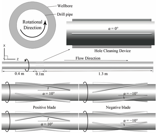
Figure 1.
Schematic of selected design parameters for the straight blade and V-shaped blade of the hole cleaning device geometry.
2.2. Governing Equations
The governing equations are described by the unsteady Reynolds averaged Navier–Stokes equations. For incompressible fluids, the mass conservation equation and the momentum conservation equation are written, as follows:
where xi is the Cartesian coordinate; ()i and ()ij represent the index tensor notion; t is the time; and denote the ensemble averaged velocity and pressure of the fluid field; gi is the acceleration of gravity; and, is the Reynolds stress term, which is related to the average velocity gradients in the following way:
in which k is the turbulence kinetic energy (TKE); δij is the Kronecker delta (δij = 1 for i = j and δij = 0 for i ≠ j); and, μt represents the turbulent dynamic viscosity, which is calculated from:
The above equations are solved using the Realizable k-ε model. It has been found that this model is more accurate than all of the k-ε models, especially for separated flows, boundary layer flows involving high-pressure gradients, and flows with complex flow structures. Thus, it is suggested that the Realizable k-ε model is suitable for the current problem [21]. The modeled transport equations for turbulence kinetic energy and its dissipation rate in the Realizable k-ε model are as follows:
where k is the TKE and ε is the dissipation rate of the TKE; σk and σε are the turbulent Prandtl numbers of the k equation and ε equation respectively; C2 is a constant; and, the generation of TKE due to the mean velocity gradients Gk is calculated as:
where S is the modulus of the mean rate of strain tensor defined as:
The coefficients that appeared in the above Realizable k–ε equations are as follows, , ; σk = 1.0, σε = 1.2, and C2 = 1.9.
One of the essential parameters in characterizing the swirl flow is the swirl number Sn, which was first proposed by Chigier and Beer [22]. It is defined as the ratio of the tangential momentum flux to the axial momentum flux, as given by:
where R1 and R0 are the radius of the drilling pipe and casing, respectively; u is the axial velocity; w is the tangential velocity; and, r is the radial coordinate. Since the swirl number is a scalar, in order to describe the rotation direction of the swirl flow using the swirl number, the sign convention of the swirl number Sn is defined, such that the Sn is positive when the rotation direction of swirl flow is consistent with the rotation direction of the blade; conversely, Sn is negative.
The decay of swirl flow can be evaluated by the decay rate β, which is the main parameter in studying the swirl flow. The decay law of swirl intensity can be expressed by the following formula:
where S0 is the initial swirl intensity and L is the distance away from the blade.
2.3. Mesh Model and Boundary Condition
The velocity inlet and pressure outlet conditions are assigned to the entrance and exits of the annulus. The nonslip boundary condition is used for the wall. Turbulence is specified regarding the intensity and hydraulic diameter of the inlet. The turbulence intensity is defined as the ratio of the root-mean-square of the velocity fluctuations to the mean velocity, which is calculated, as follows [23]:
The method of Sliding Mesh (SM) is used to simulate the rotation of the blade domain. The momentum and mass exchange between the static and rotating domains is accomplished by the interface. The mesh system is one of the major concerns in numerical simulation. To obtain the high-quality mesh system, we employ structured grids in this study. Modeling of the near wall zones is accomplished by using the standard wall function. To better capture the flow details near the blade, the meshes near the blades are refined locally, which is shown in Figure 2.
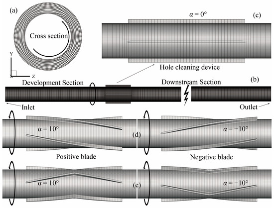
Figure 2.
The mesh structures of the hole cleaning device: (a) cross section, (b) the whole system, (c) helical angle at α = 0°, (d) positive and negative blade of the straight blade, and (e) positive and negative blade of the V-shaped blade.
2.4. Numerical Scheme
Three-dimensional and transient simulations have been carried out. The governing set of partial differential equations is a discretized utilization of the finite volume technique. The velocity and pressure fields are coupled with the Semi-Implicit Method for Pressure-linked Equation (SIMPLE) algorithm. The second order implicit scheme is used for the transient formulation. Additionally, the schemes for spatial discretization are gradient—least squares cell based, pressure—second order, momentum—second order upwind, and modified turbulent viscosity are second order upwind as well. All of the simulations are carried out at a time step of 0.001 s with 20 iterations per time step. The relative error between two successive iterations is specified through the use of a convergence criterion of 10−5 for each scaled residual component. All of the simulations in this work are performed using a workstation with the Core i7 processor and a total memory size of 16 GB RAM.
2.5. Grid Independence and Model Validation
A grid independence check was conducted over four different grid systems, 313,228, 380,228, 437,828, and 553,028 cells for a straight blade with α = 0°, and y+ was maintained at the order of unity. Table 2 shows the prediction results. The pressure drops and the mean tangential velocity at a sampling surface for the 437,828 cells grid are changed by less than 0.17% and 0.54%, respectively, as compared with the finest grid, 553,028 cells. Therefore, the 437,828 cells grid system is adopted to balance the prediction accuracy and convergence time.
Table 2.
Grid independence tests.
To assess the validity of the numerical model for the decay behavior of swirl flow, the numerical results were compared with the experimental data conducted to investigate the swirl flow from Fokeer et al. [9,24], as shown in Figure 3. In Fokeer et al.’s experiment, a 0.4 m length of the three-lobed helical pipe was installed 1.9 m downstream of the inlet cone, the strength of the induced swirling flow information, and the decay rates are quantitatively studied. The numerical model performs well with the experimental data in predicting the decaying swirl flow.
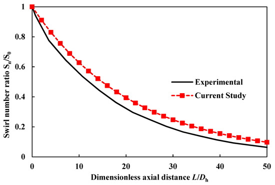
Figure 3.
Validation for present prediction with experiment results from Fokeer et al. [9,24].
3. Results
3.1. Analysis of the Effect of the Rotational Speed
Figure 4 shows the variation curve of swirl number Sn along the flow direction with four different rotational speeds (80, 120, 160, and 200 rpm) for the straight blade at α = 0°. It is noted that the initial swirl intensity S0 of the swirl flow increases with the rotational speed. For example, at 200 rpm, the initial swirl intensity S0 is 0.151, which is 2.43 times bigger than that at 80 rpm. However, the increase rate of initial swirl intensity S0 gradually decreases with the increase of rotational speed. For three different rotating speed ranges (from 80 to 120 rpm, 120 to 160 rpm, and from 160 to 200 rpm), the initial swirl intensity S0 increases by 76.2%, 47.2%, and 33.3%, respectively, when the rotational speed increases by 40 rpm.
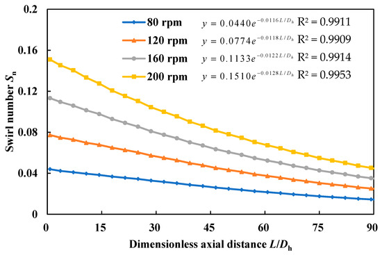
Figure 4.
Variation curve of swirl number along the flow direction with different rotational speeds for the straight blade at α = 0°.
It is shown that increasing the rotational speed can effectively improve the intensity of the swirl flow in the annulus under the condition of low rotational speed, such as 80 rpm. Additionally, an excessive rotational speed will not bring about too high swirl strength gain; however, the risk of Bottom Hole Assembly (BHA) wear and failure will increase. The swirl number Sn exponentially decays along the flow direction. This result is consistent with previous works in the literature [24,25,26]. At the same time, the decay equations of four different rotational speeds are obtained by fitting the four curves. It is known from the result that the decay rate β of swirl flow increases with the increase of rotational speed, and the decay rate β of 200 rpm is about 10.3% higher than that of 80 rpm. This phenomenon is due to the decay rate β, which is a function of the friction coefficient f, and at a high rotational speed, the swirl flow resists wall friction and the shear loss that is caused by fluid viscosity is bigger [27,28].
Figure 5 shows the tangential velocity distribution of the fluid at different cross-sections (0.41 m, 0.45 m, and 0.49 m) with different rotational speeds. Under the action of rotation, the fluid behind the suction surface of the blade obtains larger tangential velocity. The intensity of the tangential velocity and the distribution range of the fluid with a high tangential momentum increase with the increase of rotational speed, while the maximum tangential velocity can exceed 0.55 m/s at 200 rpm. At the same time, the tip leakage vortex with reverse rotation will be produced in the gap between the blade and wellbore. The intensity of the tip leakage vortex increases with the rotational speed, but it dissipates gradually along the flow direction.
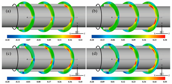
Figure 5.
Tangential velocity contours with four different rotational speeds for straight blade at α = 0°: (a) 80 rpm; (b) 120 rpm; (c) 160 rpm; and, (d) 200 rpm.
Figure 6 illustrates the tangential velocity distribution curve at z = 1.0 m with different rotational speed. It can be seen that the tangential velocity peaks in the center area and decreases gradually along the radial direction towards the wall. Near the wall, the tangential velocity rapidly decreases and then reaches zero at the wall surface. The profile of tangential velocity distribution is similar to that of a Rankine vortex. The high rotational speed will lead to greater tangential velocity in the swirling flow, and the tangential momentum transfer capacity of the flow of downstream grows with the increase of the rotational speed. Therefore, at z = 1.0 m, high rotational speed leads to a larger tangential velocity distribution at this cross-section, which significantly contributes to the removal of deposited cuttings bed.
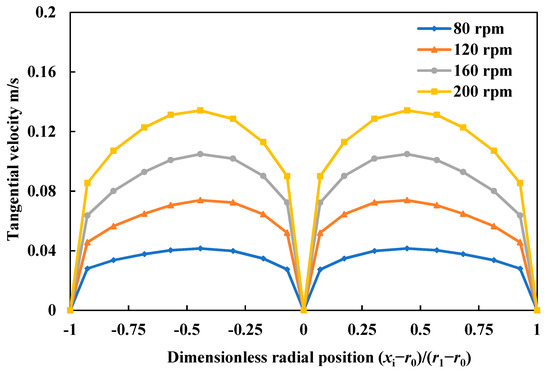
Figure 6.
Dimensionless radial profiles of tangential velocity for the straight blade at α = 0° with different rotational speeds at z = 1.0 m cross-section.
Figure 7 shows the vorticity distribution and the stream traces of the fluid at the end cross-section of the straight blade at α = 0°, with four different rotational speeds. It can be seen that under the action of the blade rotation, there will be a vortex opposite to the blade rotating direction behind the suction surface and near the wellbore wall, that is, the tip leakage vortex. This is due to the leakage of fluid through the tip clearance under the pressure difference between the pressure surface and the suction surface [29]. With the increase of rotational speed, the tip leakage vortex gradually moves to the central region of the flow channel, and the influence range of the vortex becomes small. This phenomenon is present as the tangential kinetic energy of the mainstream region increases with the increase of rotational speed. At high rotational speed, the absorption ability of the mainstream to the tip leakage vortex increases, which reduces the distribution region of the leakage vortex.
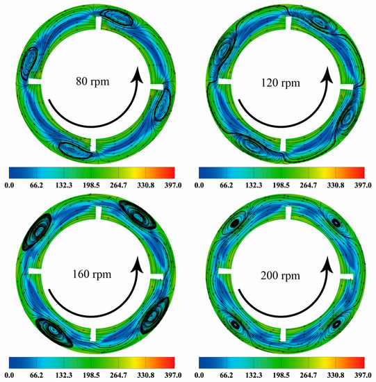
Figure 7.
Vorticity distribution and the stream traces at the end cross-section of the straight blade at α = 0° with different rotational speeds.
3.2. Analysis of the Effect of the Helical Angle
3.2.1. Influence of the Helical Angle of the Straight Blade
The helical angle is the primary structural parameter of the blade. A deflection of the axial fluid flow is caused by its variation. Figure 8 shows the curves of the swirl number Sn distribution along the flow direction with different helical angles of the straight blade at 120 rpm. It can be seen from the diagram that the swirl flow decays along the flow direction in the same exponential manner with different helical angles. The initial swirl intensity S0 decreases with the increase of helical angle for positive blades, As the helical angle α = 20° and α = 30°, the swirl number is negative, which indicates that the flow direction of the swirl flow that is induced by the blade has changed, which is opposite to the rotation direction of the blade. The initial swirl intensity S0 increases with the decrease of helical angle for the negative blades, and the negative blade is more capable of inducing swirl flow than the positive blade. It can reach S0 = 0.36 at helical angle α = −30°. The law of change in the decay rate of the positive blade is not obvious, but the decay rate of the negative blade is positively correlated with the initial swirl intensity, which indicates that the greater the intensity of the induced swirl flow, the greater the friction consumption of the resistance wall, which leads to a greater decay rate.
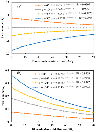
Figure 8.
Variation curve of swirl number along the flow direction for the straight blade with different helical angles at 120 rpm: (a) positive blade and (b) negative blade.
It can be seen from the performance of the positive blade that there exists a critical value in the helical angle of the blade. From a numerical point of view, when the helical angle is less than the critical value, the initial swirl intensity of the swirl flow decreases with the increase of the helical angle. Moreover, when the helical angle is greater than the critical value, the initial swirl intensity also decreases with the increase of helical angle, but the rotation direction of the swirl flow changes, which is opposite to the rotating direction of the blade. The relationship between the initial swirl intensity and helical angle that were observed are explained by the combined effect of forced deflection and blade rotation in the interaction between the fluid flow and the blade. According to the geometric model and hydraulic parameters, the critical helical angle of the positive-straight blade can be calculated, which is calculated, as follows:
where n0 is the revolutions of the blade per minute. The critical angle ψ can be calculated based on the given parameter settings of this article for ψ = 10.47°, due to, at this helical angle, the initial swirl intensity being zero. When the helical angle is close to the critical angle ψ, the flow is nearly axial, which indicates zero swirl intensity.
Figure 9 shows the relationship of the initial swirl intensity and the helical angle of the straight blade, and the fitting equation is obtained by fitting the curve. It can be seen from the diagram that the initial swirl intensity is linearly distributed with the helical angle, and the value of initial swirl intensity decreases linearly with the increase of the helical angle value. According to the fitting equation, the critical helical angle obtained is 10.91°. The difference between the fitting value and the calculated value of equation 15 is about 4.2%. The results show that it is necessary to pay attention to the design of the helical angle of the positive blade in order to ensure that the helical angle will not be close to the critical value when the drilling parameters change. Otherwise, the flow will be close to the axial flow and the application effect will be significantly reduced.
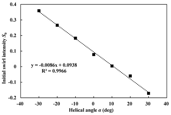
Figure 9.
Fitting curve of the relationship between helical angle and initial swirl intensity for the straight blade.
Figure 10 shows the distribution of tangential velocity at different cross-sections (0.41 m, 0.45 m, and 0.49 m) around the blade with different helical angles at 120 rpm. When the helical angle of the blade is α = 10° for Figure 10a, because the helical angle is close to the critical value, the flow is close to the axial flow, so the tangential velocity distribution is not apparent. As can be seen from Figure 10b,c, the rotation direction of the swirl flow is opposite the rotation direction of the blade due to the helical angle exceeding the critical value. At the same time, the rotation direction of the tip leakage vortex also changed due to the change of the rotation direction of the swirl flow. However, this phenomenon does not occur in negative blades configuration, as shown in Figure 10d–f. For negative blades, the tangential velocity increases with the decrease of helical angle. The maximum tangential velocity of swirl flow that is induced by the negative blade is about 2.6 times higher than that of the positive blade at the same helical angle.
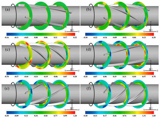
Figure 10.
Tangential velocity contours with different helical angles for straight blade at 120 rpm: (a) α = 10°; (b) α = 20°; (c) α = 30°; (d) α = −10°, (e) α = −20°, and (f) α = −30°.
Figure 11 shows the tangential velocity distribution curve of the fluid at z = 1.0 m with different helical angles. Near the critical angle of α = 10°, the tangential velocity of the fluid in this section is approximately zero, because the flow direction of the positive blade is close to the axial flow. When the helical angle is increased to α = 20° and α = 30°, the swirl intensity increases, while the rotation direction of swirl flow also changes; the maximum tangential velocity in this section can reach 0.05 m/s and 0.15 m/s. The swirl intensity of the negative blade increases with the decrease of helical angle while the rotation direction keeps the same as the rotation direction of the blades. The swirl flow that is induced by the positive blade at different helical angles at z = 1.0 m cross-section still has considerable tangential kinetic energy, and the maximum tangential velocity is around 0.3 m/s at α = −30°.
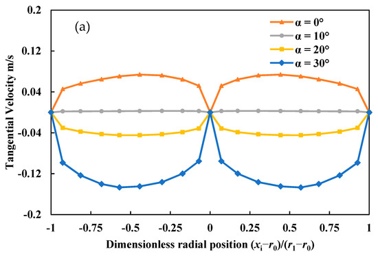
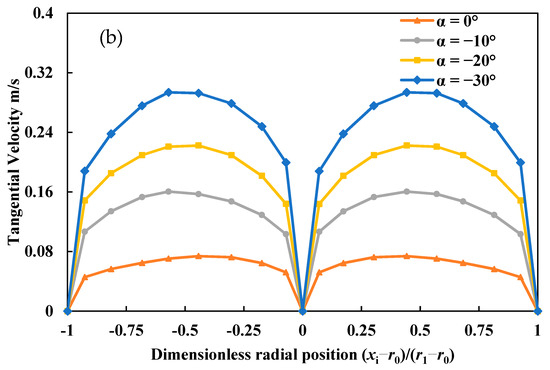
Figure 11.
Dimensionless radial profiles of tangential velocity with different helical angles for the straight blade at z = 1.0 m cross section (a) positive blade and (b) negative blade.
Figure 12 shows the vortex distribution and the stream traces at the end cross-section of the straight blade with different helical angles. It can be seen from α = 10°, α = 20°, and α = 30°, the ability of the positive blade to induce swirl flow is poor, for example, when the helical angle is α = 10°, the ability to induce the swirl flow is feeble and the central region of the flow channel is almost occupied by the tip leakage vortex. When the helical angle is α = 20° and α = 30°, with the increase of the swirl flow intensity, the influence range of the tip leakage vortex gradually becomes smaller, and the swirling effect gradually takes the upper hand. The rotation direction of the swirl flow is changed due to the deflection of the blade to the fluid. This phenomenon results in the swirl flow opposite to the direction of rotation and the tip leakage vortices in the same direction of rotation. The tip leakage vortex can also be seen in negative blades, such as for helical angle α = −10° and α = −20°, but it cannot be seen at α = −30°. With the decrease of the helical angle, the intensity and range of the tip leakage vortex decrease gradually, and finally disappear when α = −30°, which is completely absorbed by the mainstream high-intensity swirling flow.
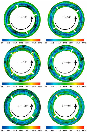
Figure 12.
Vorticity distribution and the stream traces at the end cross-section of the straight blade with different helical angles.
3.2.2. Influence of the Helical Angle of the V-Shaped Blade
Figure 13 shows the distribution of swirl number along the flow direction of the V-shaped blade with different helical angles at 120 rpm. It can be seen from the diagram that, for the positive blades, the rotation direction of the swirl flow is the same as that of the blade when the helical angle is small, such as, at α = 10°, the swirl number is positive. When the helical angle exceeds a certain angle, the rotation direction is changed to the opposite direction and the initial swirl intensity S0 decreases with the increase of the helical angle. The initial swirl intensity S0 of the negative V-shaped blade, however, decreases with the decrease of the helical angle, while its rotation direction is always opposite to that of the blade. The swirl number data versus distance under different helical angle configurations are fitted. Due to the strong ability of the negative V-shaped blade to induce swirl flow, the swirl number distribution is more consistent with the exponential law. However, the swirl number data of the positive V-shaped blade at α = 20° versus distance, it does not comply with an exponential relationship. It is suggested that the main reason for this phenomenon may be that the forced deflection of the front blade to the fluid then counteracts the relative negative pressure effect that is induced by the fluid separation of the back blade.
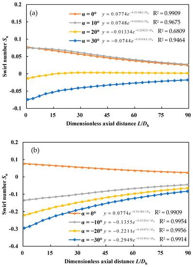
Figure 13.
Variation curve of swirl number along the flow direction for the V-shaped blade with different helical angles at 120 rpm: (a) positive blade and (b) negative blade.
The relationship between the initial swirl intensity and the helical angle of the V-shaped blade is simulated, and the fitting equation is shown in Figure 14. The results show that, when the helical angle increases from 0° to 30°, the initial swirl intensity decreases with the increase of the helical angle (absolute value) and it goes through a critical angle ψ, thus changing the rotation direction of the swirl flow. According to the fitting equation, the critical value of the positive V-shaped blade is calculated to be ψ = 18.1°, and that of the negative V-shaped blade is calculated to be ψ = 3.0°, which indicates that the critical value of the negative blade is much smaller than that of the positive blade. This is because the first segment of the positive V-shaped blade is the negative blade, and at the same helical angle, the negative blade is much more capable of inducing swirl flow than the positive blade. Therefore, the positive V-shaped blade is more capable of resisting the rotation direction change of the swirl flow, which leads to a higher critical value of the positive V-shaped blade.
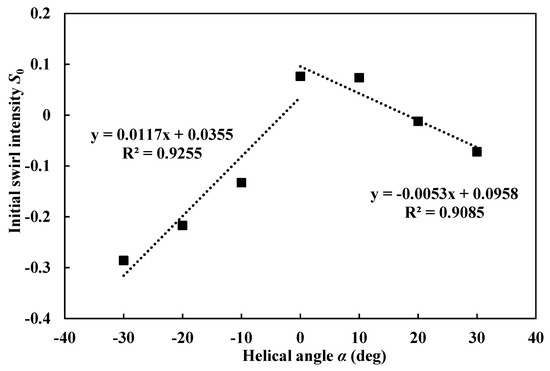
Figure 14.
Fitting curve of the relationship between helical angle and initial swirl intensity for V-shaped blade.
Figure 15 gives the tangential velocity contours with different helical angles for the V-shaped blade at 120 rpm. Thus, it is noticed that the rotation direction of swirl flow that is induced by the V-shaped blade is mostly opposite to that of rotation, while the swirl intensity at α = 10° for the positive V-shaped blade is positive. The main reason driving this phenomenon is that, when the helical angle is small, the blocking effect of the blade is weak, and the forced deflection effect of the front blade overwhelms that of the relative negative pressure effect that is induced by the block of the blade. Subsequently, the rotation direction of the swirl flow is consistent with the rotation direction of the blade under the combined effects of blocking and forced deflection. When the helical angle increases, the relative negative pressure effect induced by the block of the blade rapidly increases and exceeds the forced deflection effect. Afterwards, it leads to the rotation direction of the swirl flow, which is opposite to the blade rotation direction.
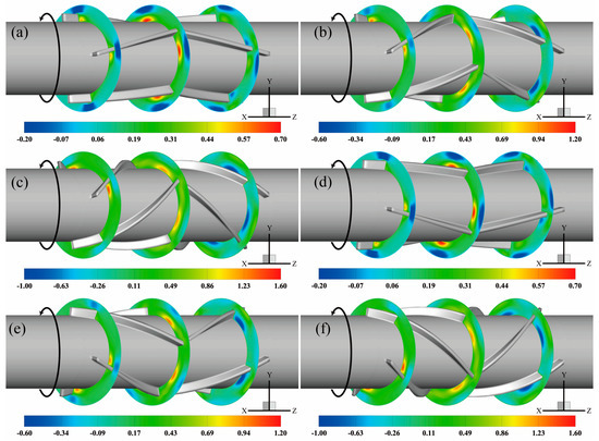
Figure 15.
Tangential velocity contours with different helical angles for V-shaped blade at 120 rpm: (a) α = 10°; (b) α = 20°; (c) α = 30°; (d) α = −10°; (e) α = −20°; and, (f) α = −30°.
Figure 16 shows the tangential velocity distribution curve of the V-shaped blade with different helical angles at the cross section of z = 1.0 m. It is known from Figure 15 that the rotation direction of swirl flow at α = 10° of the V-shaped blade is the same as the rotation direction of the blade. Thus, the rotation direction at z = 1.0 m is still positive. For the positive V-shaped blade and the negative V-shaped blade, when the helical angle increases from 0° to 30°, the relative negative pressure that is induced by the flow separation sharply increases. At the same helical angle, the tangential velocity of swirl flow that is induced by the negative V-shaped blade is greater than that of the positive V-shaped blade.
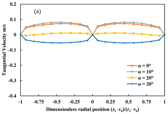
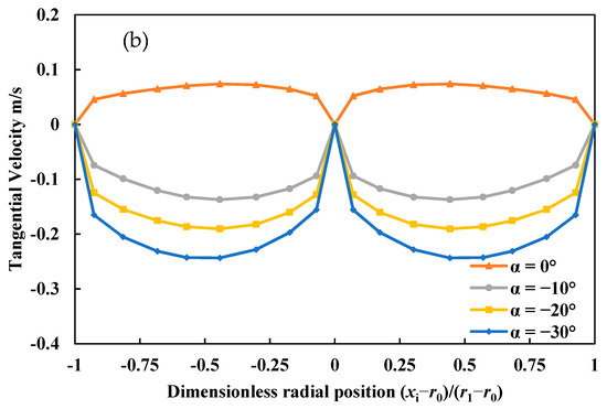
Figure 16.
Dimensionless radial profiles of tangential velocity with different helical angles for V-shaped blade at z = 1.0 m cross section: (a) positive blade and (b) negative blade.
Figure 17 shows the vorticity distribution and the stream traces at the end cross-section of the V-shaped blade with different helical angles. When compared with the straight blade that was presented previously, the swirl flow induction mechanism of the V-shaped blade is different. The swirl flow induction by the straight blade mainly depends on the forced swirl flow that is caused by the deflected flow passing the blade, while the swirl flow induced by the V-shaped blade is mainly caused by the relative negative pressure that is generated by the fluid separation under the action of inertia caused by the blockage of the blade. Under the action of V-shaped blades, there will be two kinds of eddy currents in the flow channel. One is the tip leakage vortex that is caused by the pressure difference. The other is the eddy current caused by the relative negative pressure in the flow channel that is caused by the fluid through the second stage of the blade due to the barrier of the blade and the inertia of the fluid itself. The increase of helical angle (absolute value) will increase the intensity of these two eddies, but the change of the eddy current strength caused by the latter is more obvious. At a low helical angle, the relative negative pressure effect is not strong, but the intensity and the range of eddy current in the relative negative pressure region are greatly enhanced with the increase of the helical angle (absolute value). Even the tip leakage vortex is attracted and ruptured by the relative negative pressure vortex. When the helical angle (absolute value) continues to increase, such as α = ±30°, the tip leakage vortex in the flow channel is entirely absorbed by the relative negative pressure vortex, and the rotation direction of the swirl flow will be the opposite of the rotating direction of the blade.
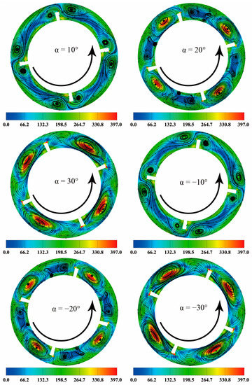
Figure 17.
Vorticity distribution and the stream traces at the end cross-section of the V-shaped blade with different helical angles.
3.3. Analysis of the Effect of the Helical Angle on Pressure Drop
Despite imposing swirl to the fluid flow, the blades of the hole cleaning device also have an undesirable effect on the pressure drop along the flow direction, which means that the losses must be considered in employing the hole cleaning device.
Figure 18 shows the variation of the pressure drop of the straight blade and the V-shaped blade with different helical angles. Variations of the pressure imply the amount of mechanical energy loss of fluid flow. Regardless of the positive blade or the negative blade, the pressure drop in the annulus will increase as the helical angle (absolute value) increases. This trend is more pronounced in V-shaped blades. This shows that the flow loss of V-shaped blade is larger than that of the straight blade with the increase of angle. However, the swirling flow induction performance of the V-shaped blade is much more feeble than that of the straight blade, which may be due to the interaction between different vortices in the vortex-induction process of V-shaped blade, which increases the energy dissipation.
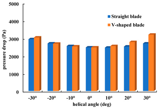
Figure 18.
Comparison of the pressure drop with different helical angles for the straight blade and V-shaped blade.
4. Conclusions
The hole cleaning devices have been used to solve the problem of cuttings accumulation during horizontal well drilling. However, under different parameters, especially under different helical angles, the intensity of swirl flow that is induced by the blade of the hole cleaning device and its decay behavior along the flow direction is not well understood. In this study, the hydrodynamic effects of different blade shape, rotational speed, and helical angle on swirl flow are numerically analyzed by CFD method. The results of the numerical simulation can provide a reference for the design of the hole cleaning device.
The initial swirl intensity increases with the rotational speed, while the increase rate of the intensity decreases with rotational speed, especially at high rotational speed. The swirl flow intensity exponentially decays along the flow direction.
Under certain parameters, there is a critical helical angle ψ for different blades. When the helical angle of the blade is close to the critical value, the swirling effect of the swirl flow induced by the blade is weak, close to the axial flow; when the helical angle is selected to exceed the critical value, the rotation direction of the swirl flow changes.
The straight blade and the V-shaped blade have different helical flow induction mechanism. The swirl flow induction by the straight blade mainly depends on the forced swirl flow that is caused by the deflected flow passing the blade, while the swirl flow induced by the V-shaped blade is mainly caused by the relative negative pressure that is generated by the fluid separation under the action of inertia caused by the blockage of the blade.
Under the same helical angle, the energy loss that is caused by V-shaped blade rotation is larger than that of the straight blade, and the larger the helical angle is, the more obvious the trend is. The V-shaped blade is weaker than the straight blade in inducing swirl flow, which indicates that the interaction between different vortices in the vortex-induction process of the V-shaped blade is more obvious, which increases the energy dissipation.
Author Contributions
This paper is the result of collaborative teamwork. J.Q. and X.S. created the numerical simulations; J.Q. wrote the paper; the numerical analysis under the supervision of T.Y.; W.L. obtained the validation; Z.L. created the visualization.
Funding
This research was funded by the National Natural Science Foundation of China (Grant No. 51474073 and Grant No. 51674087) and National Science and Technology Major Project of the Ministry of Science and Technology of China (Project No. 2017ZX05009-003).
Acknowledgments
The authors would like to express sincere appreciation to the editor and the anonymous reviewers for their valuable comments and suggestions for improving the presentation of the manuscript.
Conflicts of Interest
The authors declare no conflict of interest.
References
- Guan, Z.C.; Liu, Y.M.; Liu, Y.W.; Xu, Y.Q. Hole cleaning optimization of horizontal wells with the multi-dimensional ant colony algorithm. J. Nat. Gas Sci. Eng. 2016, 28, 347–355. [Google Scholar] [CrossRef]
- Ogunrinde, J.O.; Dosunmu, A. Hydraulics Optimization for Efficient Hole Cleaning in Deviated and Horizontal Wells. Niger. Annu. Int. Conf. Exhib. 2012, 16. [Google Scholar] [CrossRef]
- Massie, G.W.; Castlesmith, J.; Lee, J.W.; Ramsey, M.S. Amoco’s training initiative reduces wellsite drilling problems. Pet. Eng. Int. 1995, 67, 3029–3035. [Google Scholar]
- Hopkins, C.J.; Leicksenring, R.A. Reducing the risk of stuck pipe in the Netherlands. In Proceedings of the IADC/SPE Drilling Conference, Amsterdam, The Netherlands, 28 February–2 March 1995; pp. 757–766. [Google Scholar] [CrossRef]
- Oh, J.; Choi, S.; Kim, J. Numerical simulation of an internal flow field in a uniflow cyclone separator. Powder Technol. 2015, 274, 135–145. [Google Scholar] [CrossRef]
- Duangthongsuk, W.; Wongwises, S. An experimental investigation of the heat transfer and pressure drop characteristics of a circular tube fitted with rotating turbine-type swirl generators. Exp. Therm. Fluid Sci. 2013, 45, 8–15. [Google Scholar] [CrossRef]
- Varava, A.N.; Dedov, A.V.; Zakharov, E.M.; Malakhovskii, S.A.; Komov, A.T.; Yagov, V.V. Study of pressure drop and heat transfer in a swirl flow with one-sided heating in a range of heat flowrates below boiling crisis. Therm. Eng. 2009, 56, 953–962. [Google Scholar] [CrossRef]
- Lee, C.; Na, Y.; Lee, J.W.; Byun, Y.H. Effect of induced swirl flow on regression rate of hybrid rocket fuel by helical grain configuration. Aerosp. Sci. Technol. 2007, 11, 68–76. [Google Scholar] [CrossRef]
- Fokeer, S.; Lowndes, I.; Kingman, S. An experimental investigation of pneumatic swirl flow induced by a three lobed helical pipe. Int. J. Heat Fluid Flow 2009, 30, 369–379. [Google Scholar] [CrossRef]
- Derksen, J.J. Simulations of confined turbulent vortex flow. Comput. Fluids 2005, 34, 301–318. [Google Scholar] [CrossRef]
- Li, H.; Tomita, Y. Particle velocity and concentration characteristics in a horizontal dilute swirling flow pneumatic conveying. Powder Technol. 2000, 107, 144–152. [Google Scholar] [CrossRef]
- Bali, T.; Sarac, B.A. Experimental investigation of decaying swirl flow through a circular pipe for binary combination of vortex generators. Int. Commun. Heat Mass Transf. 2014, 53, 174–179. [Google Scholar] [CrossRef]
- Swietlik, G. Cutting Bed Impeller. U.S. Patent US5937957, 17 August 1999. [Google Scholar]
- Swietlik, G. Cutting Bed Impeller. U.S. Patent US6223840, 1 May 2001. [Google Scholar]
- Rodman, D.; Wong, T.; Chong, A.C. Steerable hole enlargement technology in complex 3d directional wells. In Proceedings of the SPE Asia Pacific Oil and Gas Conference and Exhibition, Jakarta, Indonesia, 9–11 September 2003. [Google Scholar]
- Puymbroeck, L.V.; Williams, H.; Drilling, V.A.M. Increasing Drilling Performance in ERD Wells with New Generation Drill Pipe. In Proceedings of the Unconventional Resources Technology Conference, Denver, CO, USA, 12–14 August 2013; pp. 1060–1070. [Google Scholar]
- Ahmed, R.; Sagheer, M.; Takach, N.; Majidi, R.; Yu, M.; Miska, S.; Rohart, C.; Boulet, J. Experimental Studies on the Effect of Mechanical Cleaning Devices on Annular Cuttings Concentration and Applications for Optimizing ERD Systems. In Proceedings of the SPE Annual Technical Conference and Exhibition, Florence, Italy, 19–22 September 2010. [Google Scholar] [CrossRef]
- Heitmann, N.; Chacinet, E.; Molero, R.; Graterol, W.; Servicios, P. Novel Integrated Hole-Cleaning Concept Reduces Well Construction by 3 Rig Days. In Proceedings of the IADC/SPE Asia Pacific Drilling Technology Conference, Bangkok, Thailand, 25–27 August 2014. [Google Scholar]
- Griffiths, W.D.; Boysan, F. Computational fluid dynamics (CFD) and empirical modelling of the performance of a number of cyclone samplers. J. Aerosol Sci. 1996, 27, 281–304. [Google Scholar] [CrossRef]
- Munson, B.R.; Young, D.F.; Okiishi, T.H. Fundamentals of Fluid Mechanics; John Wiley: New York, NY, USA, 1998. [Google Scholar]
- Araoye, A.A.; Badr, H.M.; Ahmed, W.H. Investigation of flow through multi-stage restricting orifices. Ann. Nucl. Energy 2017, 104, 75–90. [Google Scholar] [CrossRef]
- Beer, J.M.; Chigier, N.A. Combustion Aerodynamics; Applied Science Publishers LTD: London, UK, 1972. [Google Scholar]
- ANSYS Inc. Fluent User Guide and Fluent Theory Guide, Version 16.2. 2015. Available online: https://www.sharcnet.ca/Software/Ansys/16.2.3/en-us/help/flu_th/flu_th.html (accessed on 10 January 2019).
- Fokeer, S.; Lowndes, I.S.; Hargreaves, D.M. Numerical modelling of swirl flow induced by a three-lobed helical pipe. Chem. Eng. Process. Process Intensification 2010, 49, 536–546. [Google Scholar] [CrossRef]
- Li, G.; Miles, N.J.; Wu, T.; Hall, P. Large eddy simulation and Reynolds-averaged Navier–Stokes based modelling of geometrically induced swirl flows applied for the better understanding of Clean-In-Place procedures. Food Bioprod. Process. 2017, 104, 77–93. [Google Scholar] [CrossRef]
- Zhou, J.W.; Du, C.L.; Liu, S.Y.; Liu, Y. Comparison of three types of swirling generators in coarse particle pneumatic conveying using CFD-DEM simulation. Powder Technol. 2016, 301, 1309–1320. [Google Scholar] [CrossRef]
- Reader-Harris, M.J. The decay of swirl in a pipe. Int. J. Heat Fluid Flow. 1994, 15, 212–217. [Google Scholar] [CrossRef]
- Steenbergen, W.; Voskamp, J. The rate of decay of swirl in turbulent pipe flow. Flow Meas. Instrum. 1998, 9, 67–78. [Google Scholar] [CrossRef]
- Zhang, D.; Shi, W.; van Esch, B.P.M.; Shi, L.; Dubuisson, M. Numerical and experimental investigation of tip leakage vortex trajectory and dynamics in an axial flow pump. Comput. Fluids 2015, 112, 61–71. [Google Scholar] [CrossRef]


© 2019 by the authors. Licensee MDPI, Basel, Switzerland. This article is an open access article distributed under the terms and conditions of the Creative Commons Attribution (CC BY) license (http://creativecommons.org/licenses/by/4.0/).