Symmetry Detection for Quadratic Optimization Using Binary Layered Graphs

Abstract

Symmetry in mathematical optimization may create multiple, equivalent solutions. In nonconvex optimization, symmetry can negatively affect algorithm performance, e.g., of branch-and-bound when symmetry induces many equivalent branches. This paper develops detection methods for symmetry groups in quadratically-constrained quadratic optimization problems. Representing the optimization problem with adjacency matrices, we use graph theory to transform the adjacency matrices into binary layered graphs. We enter the binary layered graphs into the software package nauty that generates important symmetric properties of the original problem. Symmetry pattern knowledge motivates a discretization pattern that we use to reduce computation time for an approximation of the point packing problem. This paper highlights the importance of detecting and classifying symmetry and shows that knowledge of this symmetry enables quick approximation of a highly symmetric optimization problem.

1. Introduction

When the optimization variables can be permuted without changing the structure of the underlying optimization problem, we say that the formulation group of an optimization problem is symmetric [1,2]. For motivation, consider the circle packing problem illustrated in Figure 1 [3]. Given an integer $n>0$, the circle packing problem asks: what is the largest radius r for which n non-overlapping circles can be placed in the unit square? Costa et al. [3] show that the formulation group, i.e., a subgroup of symmetry group generated by permuting variables and constraints, is isomorphic to a symmetry group created by permuting the variable indices and switching the two coordinates in a unit square ($C_2\times S_n$). Solution methods for nonconvex optimization problems lacking symmetry-aware formulations and/or solution procedures may end up exploring all of these equivalent solutions. In other words, symmetry may cause classical optimization methods such as branch-and-bound to explore many unnecessary subtrees.

More generally, a number of authors have considered a range of symmetry detection methods, e.g., for constraint programming [4], integer programming [1,5,6,7,8], and mixed-integer nonlinear optimization [2]. These automatic symmetry detection methods can then be used to mitigate the computational difficulties caused by symmetries, e.g., with symmetry-breaking constraints [9,10,11], objective perturbation [12], specialized branching strategies [13,14], cutting planes [15,16], and extended formulations [17]. The recent computational comparison of Pfetsch and Rehn [18] indicates that these state-of-the-art symmetry handling methods expedite the solution process for the MIPLIB 2010 instances and additionally enable more instances to be solved in a time limit.

Researchers have also developed symmetry-handling methods for specific applications including covering design [19], circle packing [3,20], scheduling [21], transmission switching [22], unit commitment [23,24,25,26], and heat exchanger network synthesis [27,28]. As a concrete example of the type of contributions researchers have made, consider a job shop scheduling problem that minimizes makespan on two identical machines. Good scheduling formulations and/or solution procedures, e.g., Maravelias and Grossmann [29], Maravelias [30], and Mistry et al. [31], will implicitly exclude two of the three equivalent solutions diagrammed in Figure 2.

This paper develops detection methods for symmetry groups in quadratically-constrained quadratic optimization problems. Representing the optimization problem with adjacency matrices, we use graph theory to transform the adjacency matrices into binary layered graphs. We enter the binary layered graphs into the software package nauty that generates important symmetric properties of the original problem. Symmetry pattern knowledge motivates a discretization pattern that we use to reduce computation time for an approximation of the point packing problem.

2. Formulation Symmetry for Quadratically-Constrained Quadratic Optimization Problems

Consider the quadratically-constrained quadratic optimization problem (QCQP):

$$\begin{array}{cc}\hfill \underset{\mathit{x}\in {\mathbb{R}}^n}{min}& f_0\left(\mathit{x}\right)\hfill \\ \hfill \mathrm{s}.\mathrm{t}.& f_k\left(\mathit{x}\right)\le 0\hfill & \hfill \forall k=1,\dots ,m\\ \hfill & x_i\in \left[x_i^L,x_i^U\right]\hfill & \hfill \forall i=1,\dots ,n,\end{array}$$

(QCQP)

where:

$$f_k\left(\mathit{x}\right)=\sum _{i=1}^n\sum _{j=1}^n{\alpha }_{ij}^k{x}_i{x}_j+\sum _{i=1}^n{\alpha }_{i0}^k{x}_i+{\alpha }_{00}^k\forall k=0.\dots ,m,$$

(1)

with finite variable bounds $x_i^L,x_i^U\in \mathbb{R},\forall i$ and coefficients ${\alpha }_{ij}^k\in \mathbb{R}$ for $i,j\in \{0,\dots ,n\},k\in \{0,\dots ,m\}$.

To represent symmetry in the QCQP formulation, consider $S_n$, the symmetric group of order n formed by the $n!$ possible permutation operations. The formulation group of QCQP, or ${\mathcal{G}}_{QCQP}$, is the set of variable index permutations that preserve the objective and constraint structure [2]. For a variable index permutation $\pi \in S_n$, we seek the constraint index permutations $\sigma \in S_n$ that maintain both the objective value and the constraint structure on the feasible domain $dom\left(\mathit{f}\right)$ where $\mathit{f}=[f_1,\dots ,f_m]$. More formally:

Definition 1

(Formulation group of QCQP).

$${\mathcal{G}}_{QCQP}=\left\{\pi \in S_n\mid \forall \mathit{x}\in dom\left(f_0\right)f_0\left(\pi \mathit{x}\right)=f_0\left(\mathit{x}\right)\wedge \forall \mathit{x}\in dom\left(\mathit{f}\right)\exists \sigma \in S_m\left(\sigma \mathit{f}\left(\pi \mathit{x}\right)=\mathit{f}\left(\mathit{x}\right)\right)\right\}.$$

Because $dom\left(\mathit{f}\right)$ may be nonconvex and difficult to compute, this paper considers a ${\mathcal{G}}_{QCQP}$ restriction that enforces symmetry on the entire box bounds, i.e., we assume that $dom\left(\mathit{f}\right)=\left[{\mathit{x}}^L,{\mathit{x}}^U\right]$ for the purpose of computing ${\mathcal{G}}_{QCQP}$. The next subsections represent formulation symmetry in two ways: (i) expression graphs in Section 2.1 and (ii) tensors in Section 2.2. Representing formulation symmetry using expression graphs is due to Liberti [2] and the tensor representation is new to this paper.

2.1. Symmetry Detection with Expression Graphs

One option to compare two functions is to compare their expression trees, i.e., a directed acyclic graph representation of each function that incorporates the relevant operations, constants, and variables [2]. These expression tree models were first developed for mixed integer nonlinear optimization (MINLP) by Smith and Pantelides [32] and are common in most global MINLP solvers [33,34,35,36,37,38,39] and other MINLP-related software [40,41,42]. Figure 3 illustrates a simple example of an expression tree for $3x_1+2x_4^2+2x_2{x}_3$. A tree comparison algorithm may recursively compare two trees to determine equivalence [2]. More advanced implementations may detect equivalent but differently-formulated expressions, e.g., ${(x_1+x_2)}^2$ versus $x_1^2+2x_1{x}_2+x_2^2$.

With a directed acyclic graph representation, Liberti [2] computes the formulation symmetry group using the graph isomorphism problem, i.e., a problem that can be solved using off-the-shelf software nauty [43]. Liberti [2] also proves how to map the automorphism group of a directed acyclic graph to the formulation group of the original MINLP.

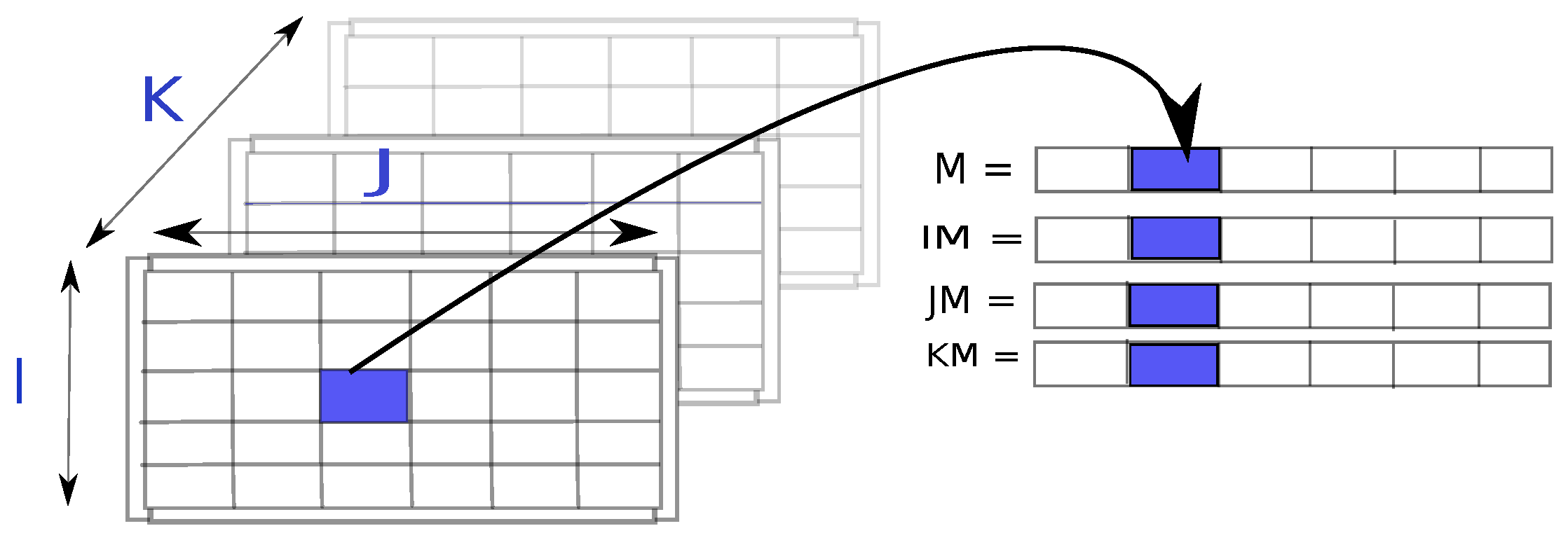
2.2. Symmetry Detection with Tensors

As an alternative to the expression tree representation, Figure 4 illustrates that QCQP can be represented as a tensor: ${\mathit{A}}_{QCQP}\in {\mathbb{R}}^{(n+1)\times (n+1)\times (m+2n)}$. Each of the two dimensions $(n+1)$ corresponds to a constant term and the variables. Each two-dimensional slice of the tensor corresponds to the constant, linear, and quadratic terms in a constraint. The first m slices correspond to Equation (1) and have entries $a_{ij}^k$. The next $2n$ slices correspond to the box constraints, i.e., $x_i\ge x_i^L$ and $x_i\le x_i^U,\forall i$.

The formulation group of this representation is:

$${\mathcal{G}}_{QCQP,T}=\left\{\pi \in S_n\mid \forall \mathit{x}\in dom\left(f_0\right)f_0\left(\pi \mathit{x}\right)=f_0\left(\mathit{x}\right)\wedge \forall \mathit{x}\in dom\left(f\right)\exists \sigma \in S_m\left({\mathit{A}}_{QCQP}(\pi ,\pi ,\sigma )={\mathit{A}}_{QCQP}\right)\right\}.$$

2.2.1. Sparse Tensor Representation

For a given tensor ${\mathit{A}}_{QCQP}$, consider a sparse representation, illustrated in Figure 5, that reduces the memory required to store the tensor. Instead of storing the entire tensor, we store arrays of length s where s is the number of nonzero entries in QCQP. The first array, $\mathit{M}$ = $(M_1,\dots ,M_s)$ stores all nonzero entries ${\alpha }_{ij}^k$ of QCQP. The next three arrays, $\mathit{I}=(I_1,\dots ,I_s),\mathit{J}=(J_1,\dots ,J_s),\mathit{K}=(K_1,\dots ,K_s)$ represent the indices corresponding to the nonzero ${\alpha }_{ij}^k$ entries. The maximum size of s is ${(n+1)}^2(m+2n)$, but, in practice, most arrays will be significantly shorter.

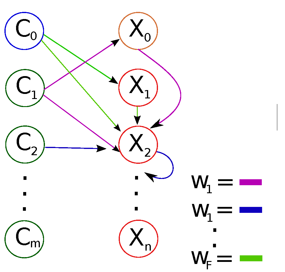
2.2.2. Converting Matrices to Edge-Labeled, Vertex-Colored Graphs

We convert the sparse tensor representation of ${\mathit{A}}_{QCQP}$ into an edge-labeled, vertex-colored graph. Given the edge-labeled, vertex-colored graph, generating graph automorphisms to the original problem symmetries is well-known [1,5,44,45]. To construct the edge-labeled, vertex-colored graph, consider a graph $G=(V,E,c)$ corresponding to an instance $\mathit{M},\mathit{I},\mathit{J},\mathit{K}$. The function $c:E\mapsto r$, for $r\in \{0,\dots ,\ell -1\}$ is an edge coloring where $\ell \in {\mathbb{Z}}^{+}$ is the number of different coefficients in $\mathit{M}$. Each unique element in $\mathit{M}$ is stored in a vector $\mathit{U}\in R^{\ell }$. We also partition (color) the vertex set into four subsets: a set $V_F$ representing the objective function, $V_C$ nodes for the constraints, a constant node $V_S$, and $V_R$ variable nodes. The automorphism definition prevents vertices from being mapped onto a vertex of a different color, so these colors prevent, for example variables becoming constraints. The equivalence relation is [2]:

$$\begin{array}{cc}\hfill \forall u,v\in V_{P}u\sim v\Rightarrow & \left(u,v\in V_F\wedge \ell \left(u\right)=\ell \left(v\right)\right)\vee \left(u,v\in V_C\wedge \ell \left(u\right)=\ell \left(v\right)\right)\hfill \\ \hfill & \vee \left(u,v\in V_S\wedge \ell \left(u\right)=\ell \left(v\right)\right)\vee \left(u,v\in V_R\wedge \ell \left(u\right)=\ell \left(v\right)\right).\hfill \end{array}$$

Figure 6 illustrates the edge-labeled, vertex-colored graph. Initially, the edge set is empty $E=\varnothing$. For $i=\{0,\dots ,s\}$ where $s=\left|M\right|$, add an edge $v_{I_i}^{\left(r\right)}$ to $v_{K_i}^{\left(r\right)}$, i.e., from a vertex in the set that represents the constant element / variables to a vertex in the set of the objective function / constraints, with the relevant color. The graph construction incorporates edges between variable nodes $V_R$ for the quadratic bilinear terms. For $i=\{0,\dots ,s\}$:

• If $I_i=J_i$, i.e., a quadratic term, then $E=E\cup \{\left\{{(v_{I_i},v_{K_i})}^r\right\}\cap \left\{{\left(v_{I_i}\right)}^r\right\}\}$.
• else for bilinear term, $I_i\ne J_i$, then $E=E\cup \{\left\{{(v_{I_i},v_{K_i})}^r\right\}\cap \left\{{(v_{J_i},v_{K_i})}^r\right\}\cap \left\{{(v_{I_i},v_{J_i})}^r\right\}\}.$

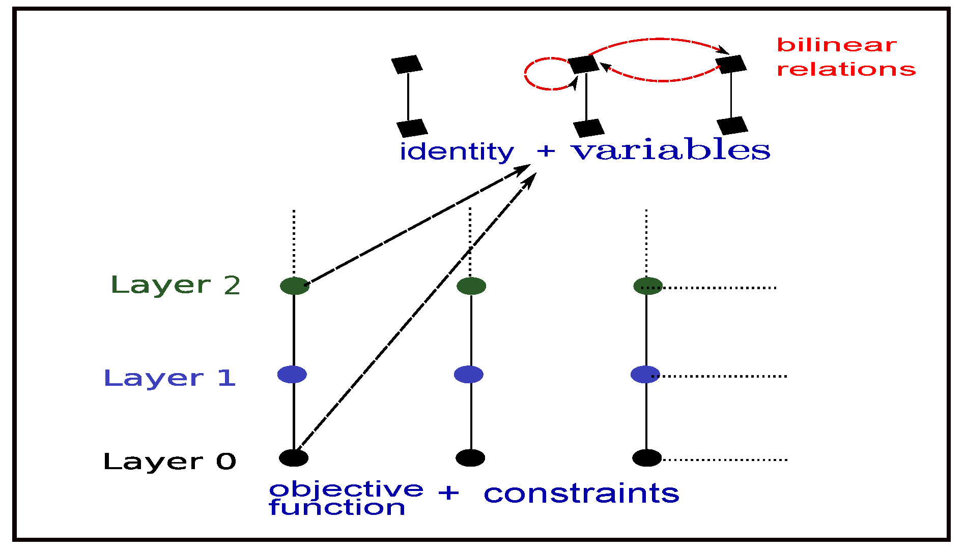
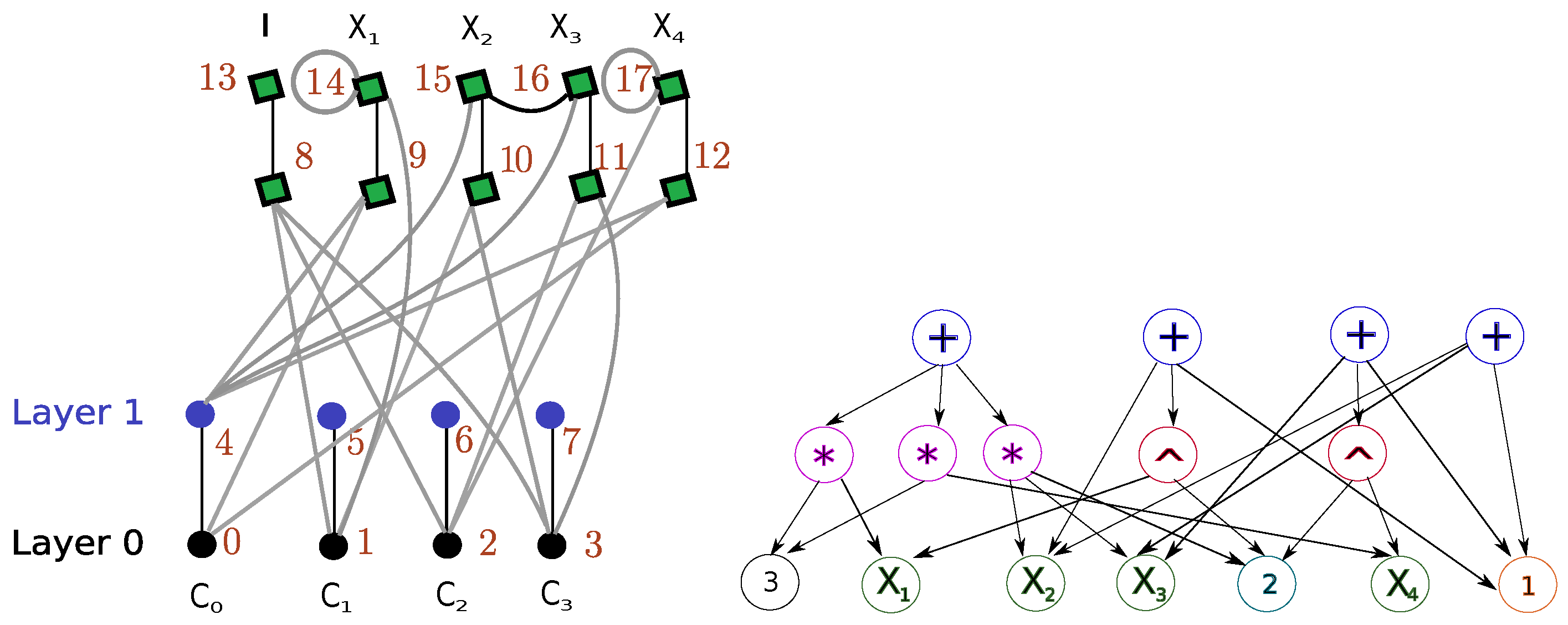
3. Formulation Symmetry Detection via Binary Layered Graphs

The software nauty [43], which detects symmetry, accepts vertex-colored graphs but does not accept the Section 2.2.2 edge-labeled, vertex-colored graphs. Thus, we associate edge colors with layers in a graph and transform the edge-labeled, vertex-colored graph into a vertex-colored graph. Since the transformation from an edge-labeled, vertex-colored graph to a vertex-colored graph is isomorphic [43], the transformation does not lose anything. Using the resulting binary layered graphs, we generate the automorphism group and find symmetry in the original QCQP.

To convert a graph $G=(V,E,c)$ with ℓ colors into an ℓ - layered graph [43], we replace each vertex $v_j\in V$ with a fixed connected graph of ℓ vertices $v_j^{\left(0\right)},\cdots ,v_j^{(\ell -1)}$. If an edge $(v_j,v_{j^{\prime }})$ has color r, add an edge from $v_j^{\left(r\right)}$ to $v_{j^{\prime }}^{\left(r\right)}$. Finally, we partition the vertices by the superscripts, $V_r=\{v_0^{\left(r\right)},\cdots ,v_{n-1}^{\left(r\right)}\}$. Alernatively, a binary representation avoids too many layers in G when the number of colors is large.

Definition 2

(Binary Layered Graph). Let $\ell \in {\mathbb{Z}}^{+}$ be the number of edge labels of G. A binary layered graph is a vertex-colored graph where the number of layers $L=\lceil {log}_2\left(\ell +1\right)\rceil$ matches a binary representation.

We assign a unique positive integer $\mu \left(z\right)$ to each $z\in \mathit{U}$ and map edge labels $\mu \left(z\right)$ to a binary representation that switches on/off parameters $c_t$ to represent the edge colors as layers. If $c_t=1$, add a new edge from $v_i^t$ to $v_j^t$ for every $c_t\in \{c_1,\dots ,c_{L-1}\}$:

$$\mu \left(z\right)=2^{L-1}·c_{L-1}\left(z\right)+2^{L-2}·c_{L-2}\left(z\right)+\cdots +2^0·c_0\left(z\right),\mathrm{for}{c}_t\in \{0,1\},t=\{0,\dots ,L-1\}.$$

(2)

Figure 7 illustrates the resulting binary labeled graph with its $L=\lceil {log}_2\left(\ell +1\right)\rceil +2$ layers. There are vertices for the objective function and each constraint and layers of copies of these constraints (connected with vertical edges). The horizontal edges encode the problem coefficients. On the upper part of Figure 7, there are vertices for a constant element and each variable and a layer of variable copies (connected with vertical edges). Here, the horizontal edges and loops distinguish the linear and bilinear terms. Algorithms 1 and 2 summarize computing the vertex and edge sets, respectively.

Algorithm 1 Algorithm constructing the vertex set

1: procedureG=($V,E$) 2:     $V\leftarrow \varnothing$, $V_s\subset V\leftarrow \varnothing \forall s$, $E\leftarrow \varnothing$ 3:     $L\in \mathbb{Z}$, $L=\lceil {log}_2\left(\left|U\right|+1\right)\rceil +2$       ▹ Define $L\in {\mathbb{Z}}^{+}$ the number of layers 4:     for $s=0\to L-3$do         ▹ Partition of vertices representing the constraints 5:         for $k=0\to m$ do 6:            $V_s\leftarrow V_s\cup \left\{v_k^{\left(s\right)}\right\}$         ▹ Copies of vertices representing the constraints 7:         end for 8:         $V\leftarrow V\cup V_s$ 9:     end for 10:     for $s=L-2,L-1$do        ▹ Partition of vertices representing the variables 11:         for $i=0\to n$ do 12:            $V_s\leftarrow V_s\cup \left\{v_i^{\left(s\right)}\right\}$        ▹ Copies of vertices representing the variables 13:         end for 14:         $V\leftarrow V\cup V_s$ 15:     end for 16:     return G 17: end procedure

Algorithm 2 Algorithm constructing the edge set

1: procedureG=($V,E$) 2:     $V\leftarrow V$ 3:     $E\leftarrow \varnothing$ 4:     for $s=0\to L-4$do                ▹ Vertical edges between copies of vertices 5:         for $k=0\dots m$do               ▹ Copies of vertices representing the constraints 6:            $E=E\cup E\cup (v_k^{\left(s\right)},v_k^{(s+1)})$ 7:         end for 8:     end for 9:                             ▹ Vertical edges between copies of vertices 10:     for $j=0\dots n$do                  ▹ Copies of vertices representing the variables 11:         $E=E\cup (v_j^{(L-2)},v_j^{(L-1)})$ 12:     end for 13:     for $F=0,\dots N-1$do                           ▹ Bilinear terms 14:         if $IM\left(F\right)=JM\left(F\right)$then                         ▹ Add a loop 15:            $E=E\cup (v_{IM\left(F\right)}^{(L-1)},v_{IM\left(F\right)}^{(L-1)})$ 16:         else 17:            if $IM\left(F\right)<JM\left(F\right)$then                         ▹ Add an edge 18:                $E=E\cup (v_{IM\left(F\right)}^{(L-1)},v_{JM\left(F\right)}^{(L-1)})$ 19:            else 20:                $E=E\cup \varnothing$ 21:            end if 22:         end if 23:     end for 24:     for $F=0\dots N-1$ do 25:         for $k=0\dots m$ do 26:            if $KM\left(F\right)=k$ then 27:                if $IM\left(F\right)=0$ then 28:                    $E=E\cup (v_k^{\left(s\right)},v_{JM\left(F\right)}^{(L-2)})$ 29:                else 30:                    $E=E\cup (v_{IM\left(F\right)}^{(L-1)},v_{JM\left(F\right)}^{(L-1)})$ 31:                end if 32:            end if 33:         end for 34:     end for 35:     return G 36: end procedure

4. Numerical Discussion and Comparison to the State-of-the-Art

The following example incorporates the algorithms proposed in this paper. We construct the binary labeled graph and then enter it into nauty through the dreadnaut command line interface:

$$\begin{array}{ccc}\hfill \underset{x_1,x_2,x_3,x_4\in [0,1]}{max}& 3x_1+3x_4+2x_2{x}_3\hfill & \hfill \left(c_0\right),\\ \hfill & x_2+{x_1}^2+1\le 0\hfill & \hfill \left(c_1\right),\\ \hfill & x_3+x_4^2+1\le 0\hfill & \hfill \left(c_2\right),\\ \hfill & x_2+x_3+1\le 0\hfill & \hfill \left(c_3\right).\end{array}$$

The optimization problem has sparse matrix representation: $\mathit{M}=(3,3,2,1,1,1,1,1,1,1,1,1),$ $\mathit{I}=(0,0,2,0,0,1,0,0,4,0,0,0),$ $\mathit{J}=(1,4,3,0,2,1,0,3,4,0,2,3),\mathit{K}=(0,0,0,1,1,1,2,2,2,3,3,3)$, vector of unique elements $\mathit{U}=[1,2,3]$, and $L=\lceil {log}_{2}4\rceil =2$ layers.

Equation (2) computes the binary representation of each unique element, e.g., $3=2^1+2^0$ indicates that there is an edge between vertices on layer zero and another edge between the same vertices on layer 1. The graph consists of four layers and $\left|V\right|=18$, one associated with a constant element and one with the objective function and the rest for the problem variables and constraints. The left-hand side of Figure 8 illustrates the graph representation. Nauty generates permutations: $\pi =(1,2)(5,6)(9,12)(10,11)(14,17)(15,16)$. To see how these Nauty-generated permutations usefully explain the symmetry properties of the entire problem, observe: (i) Permutations $(1,2)(5,6)$, as shown in Figure 8, permute the constraints $c_1,c_2$ and (ii) Permutations $(9,12)(10,11)$ are associated with the variables $x_1,x_4$ and $x_2,x_3$ with $(14,17)(15,16)$ their copies. These permutations therefore allow us to automatically calculate the formulation group $\mathcal{G}=\left(x_1{x}_4\right)\left(x_2{x}_3\right)$.

The right-hand side of Figure 8 uses Section 2.1 to develop a directed acyclic graph representation for the same problem. The graph colors represent the vertex partitioning that enables node exchanges. In this case, the directed acyclic graph representation uses a smaller number of vertices and edges than the tensor-based representation. However, the representations generate the same formulation group.

Comparison. To evaluate the trade-offs between the tensor and directed acyclic graph representations, observe that both methods will search for the same formulation group symmetries. However, the tensor representation may be especially useful when working with problems with many differently-valued coefficients, i.e., the logarithmic number of layers may reduce the number of nodes. The function assigning integer values to the problem coefficients lets us work not only with 0–1 coefficients, but also with any other value.

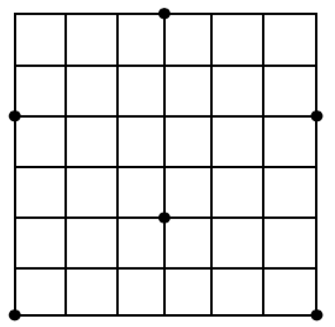
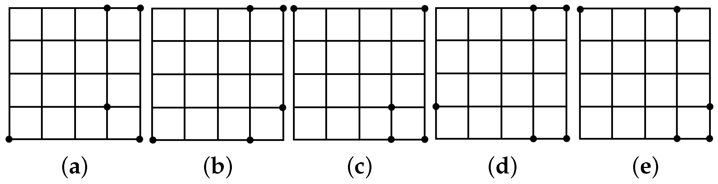
5. Exploiting Symmetry in the Point Packing Problem

Once symmetry has been detected, we can use our knowledge of the symmetry to mitigate the computational difficulties caused by symmetry. Here, we focus on solving the point packing problem [46,47,48,49]. The point packing problem concerns packing n points to a unit square. The aim is to maximize the in-between distance between any two points:

$$\begin{array}{ccccc}\hfill & \underset{}{\max }\hfill & \hfill & \theta \hfill & \hfill \\ \hfill & \mathrm{subject}\mathrm{to}\hfill & \hfill & {(x_i-x_j)}^2+{(y_i-y_j)}^2\ge \theta \hfill & \hfill 1\le i<j\le n,\\ \hfill & \hfill & \hfill & 0\le x_i\le 1,0\le y_i\le 1\hfill & \hfill 1\le i\le n,\end{array}$$

where $\theta$ denotes the minimum distance between any two points. To approximate this problem, consider a grid approach that approximates the optimal solution by adding grid lines to the unit square and forcing the points to be placed only to the vertices generated by these grid lines. Note that the point packing problem has significant applications, e.g., in placing mobile phone towers.

For n points, there will be at most a $k*\times k*$ grid, where $k*$ is the smallest number whose square is the least integer that is greater than n, i.e., ${(k*-1)}^2<n$ and $k{*}^2\ge n$. In other words, we add at most $2k*$ grid lines. On this $k*\times k*$ grid, points will occupy most of the vertexes and the unit length of spacing has been maximized. This approach, unfortunately, has the potential of missing the optimal solution. Consider fitting six points to the square. The most fitting grid is $3\times 3$ and the optimal $\theta$ we achieve is $0.5$. However, the optimal solution of $0.6009$ is achieved by the arrangement shown in Figure 9, which is not available on a $3\times 3$ grid. Although an approximation, $k*$ is still a useful pruning tool, e.g., points need to be at least $\frac{1}{k*-1}$ away from any other point.

Exhaustive Search and 2D Symmetry Removal

First, consider Algorithm 3, an exhaustive search method. To break the symmetries, start by calculating how many grids can possibly have points and the upper limit on the number of points on any occupied grid lines. Once calculated, the complete set of all possible combinations on the x-axis is calculated. For example, on a $5\times 5$ grid, one possible x-coordinate setup is $(2,0,1,0,2)$. If we label the five horizontal grid lines from 1 to 5, this setup means that there are two points on grid 1, no points on grid 2, one point on grid 3, no points on grid 4 and two points on grid 5. To remove x-axis symmetries, we consider reflections as a duplication, i.e., only one of $(1,0,2,0,2)$ and $(2,0,2,0,1)$ are considered.

Algorithm 3 Algorithm 1—Exhaustive Search

Input: number of points n, number of grids k, number of occupied grids m.      Output: The optimal solution $d^{*}$ 1: Step1 Calculate the upper bound of number of points on each occupied grid u 2: Step2 Generate complete set of combinations of x-coordinate 3: Step3 Symmetries removal on x-coordinates 4: Step4 Generate all y-coordinate sets based on binomial coefficient 5: Step5Y-coordinates pruning

Algorithm 3 considers the unique x-axis combinations. The y-axis, i.e., the horizontal grid lines, should preserve the same characteristics. Thus, in the improved Algorithm 4, we generate the set O of possible point arrangement such as $(2,0,1,0,2)$, and this is applied to both horizontal and vertical grid lines; in other words, we now consider the product $O\times O$ to give the exact coordinates of all n points.

Algorithm 4 Algorithm 2—2D Symmetry Removal

Input: number of points n, number of grids k, number of occupied grids m.      Output: The optimal solution $d^{*}$ 1: Step1 Calculate the upper bound of number of points on each occupied grid u 2: Step2 Generate complete set of combinations of x-coordinate 3: Step3 Symmetries removal on x-coordinates 4: Step4 Use the x-coordinate set to determine y-coordinate 5: Step5Y-coordinates pruning

Example 1.

Consider for five points on a $5\times 5$ grid where we have O as $\{O_1=(1,0,2,0,2),O_2=(1,2,0,0,2),$$O_3=(1,0,0,2,2),O_4=(2,1,0,0,2),O_5=(2,0,1,0,2)\}$. The finalized set of full coordinates would contain 25 elements where the product of O with itself is taken. One particular point setup generated by this approach is for example, $O_3\times O_4$. If we call the vertical grids as $V_1$ to $V_5$, respectively, and the horizontal grids as $H_1$ to $H_5$, respectively, $O_3\times O_4$ would mean that we have the following point locations:

• One point on $V_1$, 2 points on $V_4$ and 2 points on $V_5$. This is from $O_3$.
• Two points on $H_1$, 1 point on $H_2$ and 2 points on $H_5$. This is from $O_4$.

For $O_3\times O_4$, we would have five complete point setups, as shown in Figure 10. In the last setup, we have also added the labels for grids to match what we defined earlier. This diagram contains all possible arrangements of points under this particular orbit partitioning.

To improve further, we can implement pruning mechanisms such as using the bound $\frac{1}{k^{*}-1}$ to prune the non-optimal setups. In this particular example, we would have pruned all five setups as none of them satisfy the $0.5$ bound from the most fitting grid. This means that $O_3\times O_4$ is not the optimal point setup for five points on a $5\times 5$ grid.

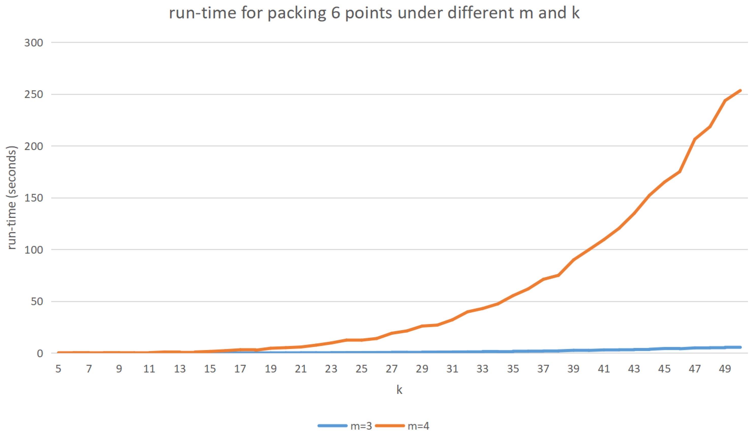
6. Results and Comparisons

Both algorithms have been implemented and run on the same devices (HP EliteDesk 800 G2 TWR Intel Core i7-6700 3.4 GHz) to provide effective comparisons. Figure 11 shows the experimental results of 2D Symmetry Removal for packing 6 points. We eliminated the result from Exhaustive Search as it is clear that 2D Symmetry Removal outperforms Exhaustive Search in terms of run-time. We notice that m, the number of occupied grids (in the diagram, this corresponds to the occupied vertical grids), has an impact on the run-time. To a reasonable extent, the larger the m, the more choices we have regarding where we place the points so it in general takes longer time to compute. Although our strategies effectively convert the point packing QCQP into a mixed-integer linear optimization problems, we could have alternatively designed a branch-and-bound algorithm that is symmetry aware.

7. Conclusions

This paper has explored alternative representations for finding symmetry in formulation groups of a quadratically-constrained optimization problem. We also show that, after knowing the symmetry, we can design significantly better methods to solve the optimization problems. The contributions in this paper are relevant to industrial problems that contain a point packing element [50,51,52].

References

1. Margot, F. Symmetry in Integer Linear Programming. In 50 Years of Integer Programming 1958–2008: From the Early Years to the State-of-the-Art; Springer: Berlin/Heidelberg, Germany, 2010; pp. 647–686. [Google Scholar]
2. Liberti, L. Reformulations in mathematical programming: Automatic symmetry detection and exploitation. Math. Program. 2012, 131, 273–304. [Google Scholar] [CrossRef]
3. Costa, A.; Hansen, P.; Liberti, L. On the impact of symmetry-breaking constraints on spatial Branch-and-Bound for circle packing in a square. Discret. Appl. Math. 2013, 161, 96–106. [Google Scholar] [CrossRef]
4. Puget, J.F. Automatic Detection of Variable and Value Symmetries. In Proceedings of the 11th International Conference on Principles and Practice of Constraint Programming—CP 2005, Sitges, Spain, 1–5 October 2005; van Beek, P., Ed.; Springer: Berlin/Heidelberg, Germany, 2005; pp. 475–489. [Google Scholar]
5. Salvagnin, D. A Dominance Procedure for Integer Programming. Master’s Thesis, University of Padua, Padua, Italy, 2005. [Google Scholar]
6. Berthold, T.; Pfetsch, M. Detecting Orbitopal Symmetries. In Proceedings of the Annual International Conference of the German Operations Research Society (GOR), Augsburg, Germany, 3–5 September 2008; Springer: Berlin/Heidelberg, Germany, 2009; pp. 433–438. [Google Scholar]
7. Bremner, D.; Dutour Sikirić, M.; Pasechnik, D.V.; Rehn, T.; Schürmann, A. Computing symmetry groups of polyhedra. LMS J. Comput. Math. 2014, 17, 565–581. [Google Scholar] [CrossRef] [Green Version]
8. Knueven, B.; Ostrowski, J.; Pokutta, S. Detecting almost symmetries of graphs. Math. Program. Comput. 2018, 10, 143–185. [Google Scholar] [CrossRef]
9. Sherali, H.D.; Smith, J.C. Improving Discrete Model Representations via Symmetry Considerations. Manag. Sci. 2001, 47, 1396–1407. [Google Scholar] [CrossRef]
10. Liberti, L. Automatic Generation of Symmetry-Breaking Constraints. In Combinatorial Optimization and Applications; Yang, B., Du, D.Z., Wang, C.A., Eds.; Springer: Berlin/Heidelberg, Germany, 2008; pp. 328–338. [Google Scholar] [Green Version]
11. Liberti, L.; Ostrowski, J. Stabilizer-based symmetry breaking constraints for mathematical programs. J. Glob. Optim. 2014, 60, 183–194. [Google Scholar] [CrossRef]
12. Ghoniem, A.; Sherali, H.D. Defeating symmetry in combinatorial optimization via objective perturbations and hierarchical constraints. IIE Trans. 2011, 43, 575–588. [Google Scholar] [CrossRef]
13. Ostrowski, J.; Linderoth, J.; Rossi, F.; Smriglio, S. Constraint Orbital Branching. In Proceedings of the 13th International Conference on Integer Programming and Combinatorial Optimization IPCO, Bertinoro, Italy, 26–28 May 2008; pp. 225–239. [Google Scholar]
14. Ostrowski, J.; Linderoth, J.; Rossi, F.; Smiriglio, S. Orbital branching. Math. Program. 2011, 126, 147–178. [Google Scholar] [CrossRef]
15. Margot, F. Pruning by isomorphism in branch-and-cut. Math. Program. 2002, 94, 71–90. [Google Scholar] [CrossRef]
16. Kaibel, V.; Peinhardt, M.; Pfetsch, M.E. Orbitopal fixing. Discret. Optim. 2011, 8, 595–610. [Google Scholar] [CrossRef] [Green Version]
17. Faenza, Y.; Kaibel, V. Extended Formulations for Packing and Partitioning Orbitopes. Math. Oper. Res. 2009, 34, 686–697. [Google Scholar] [CrossRef] [Green Version]
18. Pfetsch, M.E.; Rehn, T. A computational comparison of symmetry handling methods for mixed integer programs. Math. Program. Comput. 2019, 11, 37–93. [Google Scholar] [CrossRef]
19. Margot, F. Small covering designs by branch-and-cut. Math. Program. 2003, 94, 207–220. [Google Scholar] [CrossRef]
20. Costa, A.; Liberti, L.; Hansen, P. Formulation symmetries in circle packing. Electron. Notes Discret. Math. 2010, 36, 1303–1310. [Google Scholar] [CrossRef] [Green Version]
21. Ostrowski, J.; Vannelli, A.; Anjos, M.F. Symmetry in Scheduling Problems; Cahier du GERAD G-2010-69; GERAD: Montreal, QC, Canada, 2010. [Google Scholar]
22. Ostrowski, J.; Wang, J.; Liu, C. Exploiting Symmetry in Transmission Lines for Transmission Switching. IEEE Trans. Power Syst. 2012, 27, 1708–1709. [Google Scholar] [CrossRef]
23. Ostrowski, J.; Wang, J. Network reduction in the Transmission-Constrained Unit Commitment problem. Comput. Ind. Eng. 2012, 63, 702–707. [Google Scholar] [CrossRef]
24. Ostrowski, J.; Anjos, M.F.; Vannelli, A. Modified orbital branching for structured symmetry with an application to unit commitment. Math. Program. 2015, 150, 99–129. [Google Scholar] [CrossRef]
25. Lima, R.M.; Novais, A.Q. Symmetry breaking in MILP formulations for Unit Commitment problems. Comput. Chem. Eng. 2016, 85, 162–176. [Google Scholar] [CrossRef] [Green Version]
26. Knueven, B.; Ostrowski, J.; Wang, J. The Ramping Polytope and Cut Generation for the Unit Commitment Problem. INFORMS J. Comput. 2018, 30, 739–749. [Google Scholar] [CrossRef]
27. Kouyialis, G.; Misener, R. Detecting Symmetry in Designing Heat Exchanger Networks. In Proceedings of the International Conference of Foundations of Computer-Aided Process Operations-FOCAPO/CPC, Tucson, AZ, USA, 8–12 January 2017. [Google Scholar]
28. Letsios, D.; Kouyialis, G.; Misener, R. Heuristics with performance guarantees for the minimum number of matches problem in heat recovery network design. Comput. Chem. Eng. 2018, 113, 57–85. [Google Scholar] [CrossRef]
29. Maravelias, C.T.; Grossmann, I.E. A hybrid MILP/CP decomposition approach for the continuous time scheduling of multipurpose batch plants. Comput. Chem. Eng. 2004, 28, 1921–1949. [Google Scholar] [CrossRef]
30. Maravelias, C.T. Mixed-Time Representation for State-Task Network Models. Ind. Eng. Chem. Res. 2005, 44, 9129–9145. [Google Scholar] [CrossRef]
31. Mistry, M.; Callia D’Iddio, A.; Huth, M.; Misener, R. Satisfiability modulo theories for process systems engineering. Comput. Chem. Eng. 2018, 113, 98–114. [Google Scholar] [CrossRef]
32. Smith, E.M.B.; Pantelides, C.C. A symbolic reformulation/spatial branch-and-bound algorithm for the global optimisation of nonconvex MINLPs. Comput. Chem. Eng. 1999, 23, 457–478. [Google Scholar] [CrossRef]
33. Tawarmalani, M.; Sahinidis, N.V. A polyhedral branch-and-cut approach to global optimization. Math. Program. 2005, 103, 225–249. [Google Scholar] [CrossRef]
34. Belotti, P.; Lee, J.; Liberti, L.; Margot, F.; Wachter, A. Branching and Bounds Tightening techniques for Non-convex MINLP. Optim. Methods Softw. 2009, 24, 597–634. [Google Scholar] [CrossRef]
35. Youdong, L.; Linus, S. The global solver in the LINDO API. Optim. Methods Softw. 2009, 24, 657–668. [Google Scholar]
36. Misener, R.; Floudas, C.A. ANTIGONE: Algorithms for coNTinuous/Integer Global Optimization of Nonlinear Equations. J. Glob. Optim. 2014, 59, 503–526. [Google Scholar] [CrossRef]
37. Vigerske, S. Decomposition in Multistage Stochastic Programming and a Constraint Integer Programming Approach to Mixed-Integer Nonlinear Programming. Ph.D. Thesis, Humboldt-Universität zu Berlin, Berlin, Germany, 2013. [Google Scholar]
38. Mahajan, A.; Leyffer, S.; Linderoth, J.; Luedtke, J.; Munson, T. Minotaur: A mixed-integer nonlinear optimization toolkit. Optim. Online 2017, 6275. [Google Scholar]
39. Boukouvala, F.; Misener, R.; Floudas, C.A. Global optimization advances in Mixed-Integer Nonlinear Programming, MINLP, and Constrained Derivative-Free Optimization, CDFO. Eur. J. Oper. Res. 2016, 252, 701–727. [Google Scholar] [CrossRef] [Green Version]
40. Fourer, R.; Maheshwari, C.; Neumaier, A.; Orban, D.; Schichl, H. Convexity and concavity detection in computational graphs: Tree walks for convexity assessment. INFORMS J. Comput. 2010, 22, 26–43. [Google Scholar] [CrossRef]
41. Hart, W.E.; Laird, C.; Watson, J.; Woodruff, D.L. Pyomo: Modeling and solving mathematical programs in python. Math. Program. Comput. 2011, 3, 219–260. [Google Scholar] [CrossRef]
42. Ceccon, F.; Siirola, J.D.; Misener, R. SUSPECT: MINLP special structure detector for Pyomo. Optim. Lett. 2019. [Google Scholar] [CrossRef]
43. McKay, B.D.; Piperno, A. Practical graph isomorphism, II. J. Symb. Comput. 2014, 60, 94–112. [Google Scholar] [CrossRef]
44. Ramani, A.; Aloul, F.; Markov, I.; Sakallah, K.A. Breaking instance-independent symmetries in exact graph coloring. J. Artif. Intell. Res. 2006, 1, 324–329. [Google Scholar] [CrossRef]
45. Ramani, A.; Markov, I.L. Automatically Exploiting Symmetries in Constraint Programming. In Recent Advances in Constraints; Faltings, B.V., Petcu, A., Fages, F., Rossi, F., Eds.; Springer: Berlin/Heidelberg, Germany, 2005; pp. 98–112. [Google Scholar] [Green Version]
46. Anstreicher, K.M. Semidefinite programming versus the reformulationlinearization technique for nonconvex quadratically constrained quadratic programming. J. Glob. Optim. 2009, 43, 471–484. [Google Scholar] [CrossRef]
47. Misener, R.; Floudas, C.A. Global optimization of mixed-integer quadratically-constrained quadratic programs (MIQCQP) through piecewise-linear and edge-concave relaxations. Math. Program. 2012, 136, 155–182. [Google Scholar] [CrossRef]
48. Misener, R.; Floudas, C.A. GloMIQO: Global mixed-integer quadratic optimizer. J. Glob. Optim. 2013, 57, 3–50. [Google Scholar] [CrossRef]
49. Furini, F.; Traversi, E.; Belotti, P.; Frangioni, A.; Gleixner, A.; Gould, N.; Liberti, L.; Lodi, A.; Misener, R.; Mittelmann, H. QPLIB: A library of quadratic programming instances. Math. Program. Comput. 2019, 11, 237–265. [Google Scholar] [CrossRef]
50. Jones, D.R. A fully general, exact algorithm for nesting irregular shapes. J. Glob. Optim. 2014, 59, 367–404. [Google Scholar] [CrossRef]
51. Misener, R.; Smadbeck, J.B.; Floudas, C.A. Dynamically generated cutting planes for mixed-integer quadratically constrained quadratic programs and their incorporation into GloMIQO 2. Optim. Methods Softw. 2015, 30, 215–249. [Google Scholar] [CrossRef]
52. Wang, A.; Hanselman, C.L.; Gounaris, C.E. A customized branch-and-bound approach for irregular shape nesting. J. Glob. Optim. 2018, 71, 935–955. [Google Scholar] [CrossRef]
Figure 1. Given an integer n > 0 , the circle packing problem asks: what is the largest radius r for which n non-overlapping circles can be placed in the unit square? Already for n = 2 , there are four equivalent solutions [3]; these solutions are related to one another via rotations and reflections.
Processes 07 00838 g001
Figure 2. To observe symmetries that may arise in scheduling, consider a job shop scheduling problem that minimizes makespan on two identical machines. Lacking symmetry-aware formulations and/or solution procedures, a solution procedure may end up exploring all three of these equivalent solutions.
Processes 07 00838 g002
Figure 3. Example of an expression tree for 3 x 1 + 2 x 4 2 + 2 x 2 x 3 .
Processes 07 00838 g003
Figure 4. Tensor representation of the symmetry.
Processes 07 00838 g004
Figure 5. Sparse tensor representation models A Q C Q P as 4 arrays with the nonzero entry α i j k in M and arrays I , J , K holding the index.
Processes 07 00838 g005
Figure 6. The tensor A Q C Q P as an edge-labeled, vertex-colored graph.
Processes 07 00838 g006
Figure 7. Binary layered graph representation of QCQP using the tensor representation A Q C Q P .
Processes 07 00838 g007
Figure 8. Illustration of the example problem using the binary labeled graph representation (left) and the directed acyclic graph representation (right).
Processes 07 00838 g008
Figure 9. Optimal arrangement of six points.
Processes 07 00838 g009
Figure 10. Five point setups for O 3 × O 4 . (a) point setup1; (b) point setup2; (c) point setup3; (d) point setup4; (e) point setup5.
Processes 07 00838 g010
Figure 11. Run-time for six points on different grids with different number of occupied grids. The line m = 4 is above the line m = 3 .
Processes 07 00838 g011