1. Motivation
This paper addresses the design of locally optimal experimental plans for liquid–liquid equilibria (LLE) characterization. For a systematic handling of the problem, we propose semidefinite programming (SDP) formulations combined with the Model-based Optimal Designs of Experiments (M-bODE) using thermodynamic models for forecasting the equilibria. The innovations of the paper are twofold: (i) presenting a systematic approach based on mathematical programming strategies to handle the optimal design of experiments for LLE characterization; and (ii) addressing the difficulties in model-based optimal designs of experiments for models described by implicit nonlinear algebraic equations including the factors, the measurements and the parameters to be estimated. Typically, the statistics community focuses on M-bODE for models described by explicit algebraic equations where the measurements are related to the experimental factors and the parameters. The generalization to implicit nonlinear models was, as far as we know, not previously considered. The novelty lies in the computation of the parametric sensitivities which, for the LLE problem, require solving a linear system of equations.
Liquid–liquid extraction is an important separation unit operation that finds application in a variety of areas of the chemical process industries, including those for petrochemicals, food, and pharmaceuticals. Accurate phase equilibrium data are important for the design and optimization of industrial plants for extraction processes. Moreover, ternary systems equilibrium data are essential for the proper understanding of the solvent extraction process and so for solvent selection. Typically, characterizing the LLE for ternary mixtures requires complex experimental plans to obtain data for subsequently fitting thermodynamic models able to simulate and optimize unit operations [
1]. Several methods can be used to obtain LLE data [
2] but in most cases the task requires considerable resources, both human and economic. The building of adequate mathematical models from LLE data typically involves:
- (i)
choosing the appropriate thermodynamic model according to the nature of the mixture and the region of operation;
- (ii)
defining the methodology to estimate parameters that are able to describe well the experimental data;
- (iii)
iterative computation of LLE and stability analysis to prevent spurious phase predictions;
- (iv)
refinement of existing models, by planning further experiments; and
- (v)
designing experiments prior to the laboratory experiments.
While Items (i)–(iii) are extensively studied in literature, Items (iv)–(v) are scarcely tackled in the context of chemical thermodynamics. The main reasons are that the models are of large complexity and include highly nonlinear terms. This study contributes to filling the gap detected.
The approach proposed herein requires an approximated knowledge of the binary interaction parameters (BIPs), which can be obtained from data in the literature for similar components to those in the mixture of interest or estimated from group contribution methods, such as UNIFAC. In addition, a prior knowledge is required of the number of immiscible pairs of components in the ternary system, i.e., its type. Using this information, the method is capable of calculating a locally optimal experimental design. The experimental results either will confirm the estimates of the initial BIPS, or will update their values. In the latter case, the method finds another optimal experimental design, now based on the updated BIPs. The method is thus: (i) used for parameter confirmation; or (ii) included in a sequential procedure where the parameters are iteratively refined.
M-bODE generates efficient plans of experiments for parameter estimation and has currently gained importance due to the necessity of judiciously choosing the most informative experiments, given the budgetary constraints on resources. M-bODE thus allows important cost savings in scientific studies by determining the most efficient designs for accurate inference [
3].
It is a matter of surprise that M-bODE is not reported for generating experimental plans for LLE characterization. The exception is the work of Dechambre et al. [
4], who proposed a strategy combining the discretization of the initial mixture space with an algorithm similar those of the classic exchange methods [
5,
6,
7].
Among the classic approaches, various numerical algorithms based on exchange methods [
5,
8,
9] have been developed for the construction of optimal experimental designs. These algorithms are iterative, requiring a starting design and a stopping criterion in the search for the optimal solution. They iteratively replace current design points by one or more points that may be either new or already in the support of the current design. The rule for selecting the point or points for generating the next design vary depending on the type of algorithm and the design criterion. The numerical efficiency of these Wynn–Fedorov schemes has been improved by several authors, including Wu [
10], Wu and Wynn [
11], Pronzato [
12] and Harman and Pronzato [
13]. They were reviewed and compared by Meyer and Nachtsheim [
14] and Pronzato [
15], among others. Another approach to finding continuous optimal designs is based on Multiplicative algorithms, which have found broad application due to their simplicity [
16]. The basic algorithm was proposed by Titterington [
17] and later exploited by Pázman [
18], Fellman [
19], Pukelsheim and Torsney [
20], Torsney and Mandal [
21], Mandal and Torsney [
22], Dette et al. [
23], Torsney and Martín-Martín [
24], Yu [
25], and Yu [
26]. Recently, cocktail algorithms, which rely on both exchange and multiplicative algorithms, have been proposed [
27]. Another algorithm falling in the same class was proposed by Yang et al. [
28] where the iterative procedure includes a Newton method-based solver for determining the weights given a set of support points and an optimization step where the dispersion function is maximized by choosing the set of support points. All these approaches find the optimal discrete set of design points constructed from the original continuous design space.
We also discretize the initial mixture domain to produce a set of candidate one-point experiments, but instead propose a mathematical programming (MP) based approach to determine the relative weights of individual one-point experiments (most weights will be zero). Mathematical programming approaches have been successfully applied to solve many design problems. Some examples are Linear Programming [
29,
30], Second Order Conic Programming [
31,
32], Semidefinite Programming (SDP) [
33,
34,
35], Semi-Infinite Programming (SIP) [
36,
37], Nonlinear Programming (NLP) [
38,
39], NLP combined with stochastic procedures such as genetic algorithms [
40,
41], and global optimization techniques [
42,
43]. They are particularly efficient for
approximate (also called
continuous) optimal designs, characterized by a continuous representation of the weights of each constituent one-point experiment in the plan; the design problem has convex properties and the quality of the optimum can be checked with a General Equivalence Theorem (GET). Moreover, the resulting optimization problem can be solved efficiently using state-of-the-art solvers that guarantee global optimality, especially when the optimization problem belongs to a convex programming class.
It is important to emphasize that most of the MP-based formulations listed above are for
explicit models where by “explicit models” we refer to functional forms that explicitly relate the response variables and the control factors. Contrarily, in this study, we address
implicit models which are functionals of nonlinear type relating the responses, control factors and parameters; a classic example is the LLE thermodynamic model [
44]. As far as we know, the use of classic approaches to handle implicit models is not reported in the literature because of the additional complexity of computing the parametric sensitivity. In practice, MP-based approaches are more suitable for this class of models since the construction of the FIM can be embedded in the formulation for finding the optimal design. MP-based approaches are also advantageous in finding
constrained optimal designs, where additional constraints on the distribution of weights are explicitly included in the formulation. Finally, the mathematical programming problems falling into convex formulations (as is the case of SDP formulations), guarantee the global optimality of the obtained design for the chosen discrete set of candidate points. The classic algorithms lack such a proof.
A disadvantage of MP-based methods is that the size of the optimization problem increases almost exponentially with the number of candidate points. The solvers may take larger computational times than those required by classic algorithms and may even not converge for problems of large dimension. However, the current SDP solvers based on interior point methods can efficiently handle problems with 1 × 10
4 constraints [
35].
Paper Organization and Nomenclature
Section 2 presents the mathematical representation of the LLE model, the background required for applying the methods of optimal experimental design and the fundamentals of SDP.
Section 3 formulates the optimal design of experiments for an SDP solution, covering the details of: (i) FIM construction; and (ii) computational implementation.
Section 4 applies the proposed formulations to systems of Type 1, which are the most common in liquid–liquid extraction processes; for the classification of LLE systems topology, see Treybal [
45]. Two different classes of ternary system of Type 1 are considered for demonstration purposes: (i) Class I, where Components 2 and 3 are completely miscible but Components 1 and 2 and 1 and 3 are both partially miscible; and (ii) Class II, where Components 1 and 3 and 2 and 3 are completely miscible but Components 1 and 2 are only partially miscible ([
46], p. 8.163).
We use bold face lowercase letters to represent vectors, bold face capital letters for continuous domains, blackboard bold capital letters for discrete domains, and capital letters for matrices. Finite sets containing elements are compactly represented by . The symbol “” is used to indicate the vector/matrix transpose operation, stands for the trace of a matrix and for the cardinality of a discrete set.
2. Background
This section provides the background material required by the mathematical formulation for obtaining approximate optimal designs for LLE characterization. First, we introduce the model used to describe the LLE for ternary systems (
Section 2.1). Next, the basic theory of model-based optimal designs of experiments is provided (
Section 2.2), and
Section 2.3 introduces the fundamentals of SDP.
2.1. Liquid–Liquid Equilibria: Mathematical Representation
We first present the model relating the compositions of each component of a ternary mixture in each phase. The LLE characterization studies are performed at constant pressure and temperature. Let be the set of components in the mixture, and the set of phases into which the original mixture separates. Consequently, , such that and . The set of candidate experiments is formed by a finite number () of vectors , i.e., . The compositions of the components in each phase are denoted by where the first subscript identifies the phase, , and the second is for the component, . Similarly, in each phase and ignoring any measurement errors, the component fractions sum to 1, i.e., and .
The LLE model includes mass balances and the equilibrium conditions relating the compositions of the components in both phases. Here, we assume the equilibrium of chemical potentials which translate into iso-fugacity relations. The activity coefficient, here denoted by
, is determined using the Non-random Two-liquid (NRTL) model [
47], but without loss of generalization other models such as the Universal Quasichemical (UNIQUAC) model [
48] and the UNIQUAC Functional-group Activity Coefficients (UNIFAC) model [
49] can be used. The vector of parameters in the model,
, includes the dimensionless pair of interaction parameters,
, in turn related to the interaction energy parameters, and the non-randomness parameters,
. Consequently, in this study, we have
. For ternary systems,
is a
matrix containing the interactions between all the pairs of components in the mixture. Since the interaction energy of each species with itself is null, corresponding to
for
, the complete set of parameters to be estimated from the proposed experimental plan includes six pairs of interaction parameters,
. Similarly,
is a symmetric
matrix, where the elements on the diagonal are 0, and
. For ternary systems, the number of additional parameters
is three. However, in some of the experimental plans, we assume
fixed having a value in the interval
(see Rappel et al. [
50] among others) and focus only on the determination of the parameters
. Summing up, if the experimental plan aims at finding only the pairs of interaction parameters,
includes six
s, i.e.,
. Otherwise, if the goal is estimation of the pair interaction parameters and the pairs of non-randomness parameters,
includes six
s and three
s, i.e.,
. The calculation of designs for both cases is demonstrated in
Section 4.
The LLE model is compactly written in the form where is a set of nonlinear algebraic equations:
Equation (1a) represents the iso-fugacity constraints for all the components, Equation (1b) is for the summation of the component fractions in each phase after separation, and Equation (1c) is the mass balance for the second component obtained by applying the lever rule. Alternatively, Equation (1c) can be replaced by the mass balance for the third component, corresponding to
. The activity coefficients
, are modeled by the NRTL model presented in
Appendix A. For compactness,
represents the vector of compositions of the components in the
pth phase. Note that: (i) the link between the equilibrium composition and that of the initial mixture is Equation (1c) but the equilibrium can only be fully characterized after solving all equations in Equation (1) together; and (ii) by assumption
.
Typically, an experiment to characterize LLE requires choosing an initial mixture, , providing a separation in two phases is obtained, and measuring at least the composition of two components in each phase, e.g., Components 1 and 2. The measurement errors of all four variables are assumed independent and identically distributed with mean zero and constant variance.
2.2. Optimal Design of Experiments
The regression models addressed herein are described by
and have a four-variate response with two independent variables (covariates) used to set the initial mixture composition, e.g.,
and
. The remaining fraction is dependent on the first two so that
. The mean response at
is
where
and
solve Equation (1) for a given
. Here,
where
is a compact domain containing the parameters values and
is the expectation operator with respect to the error distribution.
Because the model is nonlinear, the FIM is dependent on the values of
to be estimated from the experimental design. Here, we address
locally optimal designs [
51] where the model parameters are taken from previous studies or experiments and they are then treated as known in the FIM construction. We note that this framework is particularly useful when a good estimate is available and the study serves to confirm parameter estimates or is a step of a sequential design (see Atkinson et al. [
52]).
In this study, we focus on
approximate designs,
, which allocate a weight
to
ith candidate experiment
, with
. The weights
can also be interpreted as the relative effort put on initial mixtures
, and many of them may be null in the optimal design if the additional information provided by the corresponding mixtures is low (or none). In practice, approximate designs are implemented by taking roughly
replicates at mixture
after rounding
to an integer subject to the constraint
where
k stands for the number of support point of the optimal design. Advantages of working with continuous designs are many, and there is a unified framework for finding optimal continuous designs for M-bODE problems when the design criterion is a convex function on the set of all approximate designs [
53]. In particular, the optimal design problem can be formulated into a mathematical optimization program with convex properties and equivalence theorems are available to check the optimality of a design. In many algorithms for finding optimal designs, the number
k of support points has to be specified by the experimenter, with comparisons between designs for different
k leading to the optimal value. However, in our formulation, the optimal value of
k is part of the output of the algorithm and is found solving the problem using SDP. Rounding procedures for exact designs can be found in the work of Pukelsheim and Rieder [
54].
We identify the set
of all feasible approximate designs in
as the
-dimensional simplex in the space of weights satisfying
. An optimal experimental design is represented by a
k-tuple
where
k candidate one-point designs have
. Here, the first three lines are for the compositions in the initial mixture and the fourth for the weight of this candidate experiment. The corresponding equilibrium compositions in both phases are stored in a
-tuple
where each column contains the compositions in each phase after separation for each one-point design forming the optimal design. The second subscript of
y is to identify the support point while the first is for phase.
The performance of the design
is measured by a convex functional of its FIM. The elements of the normalized FIM obtained after adjusting for the sample size are the negatives of the expectation of the second-order derivatives with respect to the parameters of the log-likelihood of Equation (2) for component
j in phase
p given the set of candidate treatments
, denoted as
. This matrix is proportional to
where
is the FIM from the design
considering a single measurement—the composition of
jth component in phase
p, i.e.,
.
is the corresponding
elemental FIM from point
. The
global FIM including all four responses is obtained summing up the FIMs
weighted by the variance–covariance matrix for the corresponding pair of observations [
55,
56], i.e.,
Here, we assume that the measurements are independent, which implies that the variance–covariance matrix is diagonal. Additionally, by assumption, all the measurements have the same error variance, which yields an equally weighted sum in Equation (4), i.e., .
When errors are normally and independently distributed, the volume of the confidence region for the model parameters
is inversely proportional to
. Consequently, maximizing the determinant of the FIM, by choice of a design leads to the most accurate estimates for the parameters. If the interest is in finding the approximate D-optimal design, the optimization problem is
Other design criteria optimize the FIM in different ways. For example, if the formulation is used to find A-optimal designs, the optimization problem is
and, if the objective is finding E-optimal designs, the optimization problem is
where
stands for the minimum eigenvalue of •. To check the optimality of the designs found, we use the equivalence theorems [
52,
57]. The scaled
sensitivity function,
, for a point
is given by
where
is the vector of sensitivities at
, and
is the eigenvector of
corresponding to
. The sensitivity function in Equation (8) is limited from above by 0, and achieves the maximum at the support points.
2.3. Semidefinite Programming
In this paper, semidefinite programming is employed to solve the optimal design problems for D-, A- and E-optimality criteria over a given discrete domain . In this section, we introduce the fundamentals of this class of mathematical programs.
Let
be the space of
symmetric positive semidefinite matrices, and
the space of
symmetric matrices. A convex set
is semidefinite representable (SDr) if
, interpreted as the projection
on to a higher dimensional set
, can be described by Linear Matrix Inequalities (LMIs). That is,
is SDr if and only if there exists some symmetric matrices
such that [
58]
Here, ⪰ is the semidefinite operator, i.e., , where is the Frobenius inner product operator, is a point of the original set , and is a point of the incremental dimensional subspace.
In turn, a convex (or concave) function
is SDr if and only if the epigraph of
,
, or the hypograph,
, respectively, are SDr and can be casted by LMIs [
59,
60]. The optimal values,
, of SDr functions are then formulated as
semidefinite programs of the form
In our design context, is a vector of known constants that depends on the design problem, and matrices contain local FIMs and other matrices produced by the reformulation of the functions into LMIs. The decision variables in vector are the weights , of the optimal design and other auxiliary variables required. The problem of calculating a design for a pre-specified set of candidate experiments of points , is solved with the formulation in Equation (10) complemented by the linear constraints on : (i) ; and (ii) , where is a unitary column vector with lines. The problem in Equation (10) is the classic SDP problem which includes LMIs representing conic constraints.
Ben-Tal and Nemirovski [
59] provided a list of SDr functions useful for solving continuous optimal design problems with SDP formulations (see Boyd and Vandenberghe [
60], Section 7.3). Recently, Sagnol [
61] showed that each criterion in the Kiefer class of optimality criteria defined by
is SDr for all rational values of
and general SDP formulations exist for them. This result also applies to the case when
; the problems in Equations (
5)–(
7) fall into this class. Practically, the problem of finding optimal approximate plans of experiments for the most common (convex) criteria can be formulated as a semidefinite programming problem falling into the general representation (
9) (see Vandenberghe and Boyd [
33] and Duarte and Wong [
35] among others).
3. SDP Formulations for Finding Optimal Design of Experiments
This section presents the formulations for finding approximate optimal designs via SDP. First, we introduce the approach used for calculating the FIM (see
Section 3.1). In
Section 3.2, we introduce the SDP formulations for finding approximate D-, A- and E-optimal designs for the LLE model, and
Section 3.3 covers implementation aspects.
3.1. FIM Construction
This section describes the procedure used to construct the global FIM for a candidate initial mixture
. We recall the model in Equation (1) is formed by six algebraic equations with general form
where
. The model derivation with respect to the parameters leads to
where
denotes the sensitivity of the measurement
to parameter
with
defined in
Section 2.1. The resulting set of linear algebraic Equation (12) can be cast as
where
F is the
matrix formed by terms
, and
b is a column vector of size
containing the terms
. Consequently, the solution of Equation (13) is obtained inverting
F, i.e.,
Now, the elemental FIM’s can be generated using the relation
which enables the computation of the matrices
and
using Equations (
3) and (
4), respectively. In case the matrix
is singular, the strategies proposed by Shahmohammadi and McAuley [
62] can be employed.
3.2. SDP Formulations for D-, A- and E-Optimal Designs
This section presents the formulations for finding optimal designs via SDP. The D-optimality criterion is addressed first. Next, the formulations for A- and E-optimal design problems are introduced.
Here, we recall the approximate D-optimal design problem in Equation (5), and use the formulation proposed by Vandenberghe and Boyd [
33] to handle the problem. That is, given the LLE model, the set of local parameters, the set of candidate experiments
(already generated), the
elemental FIMs for each candidate experiment and the total number of experiments
, the formulation for finding approximate D-optimal designs on
may be formulated as follows:
where Equation (16a) is the objective function, Equation (16b) assures the semidefinite positiveness of the global FIM, Equation (16c) is for the global FIM equality, Equation (16d) generates the FIMs for each measurement, Equation (16e) represents the semidefinite positiveness of
, and Equation (16f) guarantees that the weights sum to 1. Here,
is a
matrix of zeros. Similarly, the formulation for the A-optimality criterion introduced in Equation (6), is as follows:
where the difference is solely in the objective function. Finally, for the E-optimal design problem presented in Equation (7), the formulation is
3.3. Implementation Aspects
In this section, we detail the computational implementation of the procedure for finding optimal designs for LLE experiments.
The nonlinear algebraic equations in Equation (1) are solved for each candidate mixture
using a Newton–Krylov–Armijo algorithm. The solver uses the Krylov method for computing Newton inexact directions and the Armijo rule to globalize the Newton method (see Kelley [
63]). The relative and absolute tolerances used in the solver are 1 × 10
−7 and 1 × 10
−8, respectively.
The set of candidate experiments is constructed using an equidistributed grid in both coordinates and . An equal step is used for both and all the points satisfy the condition . Finally, is computed as .
Both derivatives in Equation (12) (
and
) are determined via automatic differentiation using
ADiMat code [
64].
To handle the SDP problems in Equations (16)–(18), there are user-friendly interfaces, such as
cvx [
65] or
Picos [
66], that automatically transform the semidefinite constraints in Equations (16b) and (16e) and the objective functions into a series of LMIs before passing them to SDP solvers such as
SeDuMi [
67] or
Mosek [
68]. This is possible when
is SDr, which is true for our design criteria. In our work, we solved all SDP problems using the
cvx environment combined with the solver
Mosek that uses an efficient interior point algorithm [
69].
To check the optimality of the designs found, we compute the scaled sensitivity function for every initial mixture using Equation (8). From this set of values, we extract the maximum, that, practically, corresponds to a support point. The values of the scaled sensitivity function of the other support points, here denoted as , are also used for comparison and we require that , where is the minimum threshold allowed and was set to −0.02. The rational for choosing the value of is that we require approximate designs with at least 98% efficiency.
All computations in this paper were carried using on an Intel Core i7 machine (Intel Corporation, Santa Clara, CA, USA) running 64 bits Windows 10 operating system with . The relative and absolute tolerances used to solve the SDP problems were set to 1 × 10⁻⁵ in all problems.
4. Results
In this section, we apply the formulations of
Section 3.2 to find locally D-, A- and E-optimal designs for LLE characterization. We consider three examples to demonstrate the approach: In the first two examples, the set of parameters to be estimated from the experiments is only the vector of dimensionless binary interaction parameters, i.e.,
, which is six parameters. We consider two ternary systems to demonstrate that the strategy can be applied to Type 1 systems of Class I (
Section 4.1) and Class II (
Section 4.2). Finally, we present an example where the non-random binary interaction parameters are also included in the set of parameters to be estimated, i.e.,
, thus there are nine parameters (see
Section 4.3).
A generalization of the method for systems of Type 2 (with delamination in two binary subsystems) and of Type 3 (with delamination in all three binary subsystems) requires the adaptation of the strategy to the specificities of the system. However, the strategy to follow is similar and involves: (i) experiments of mutual solubility of immiscible pairs of components; (ii) determination of binodal points by successively adding the third component; and (iii) the determination of the tie-lines where the LLE is characterized at different compositions of the ternary mixture. The proposed method can be similarly used to assist the laboratory work in Step (iii) with Steps (i) and (ii) used to generate prior knowledge.
In all examples, the initial grid of mixtures result from equistributing the points with a constant interval in the composition domain . In all examples, we use ; the complete set of candidate experiments is populated with 66 mixtures. Naturally, other step sizes can be used. Typically, the CPU time required by the SDP solver increases as the grid becomes finer, but the solver can efficiently tackle problems including thousands of LMIs.
All designs presented in following paragraphs were submitted to optimality checking employing the approach described in
Section 3.3. All of them guarantee scaled sensitivity values at the support points below 2%, which allows inferring they are nearly optimal for practical implementation.
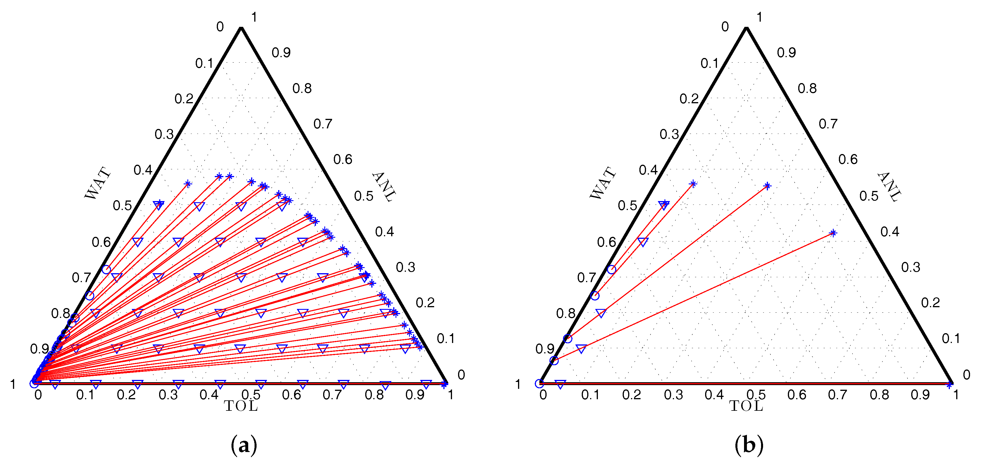
4.1. Example 1—Ternary System of Type 1, Class I; Including Dimensionless BIPs
First, let us consider that
only includes the dimensionless binary interaction parameters and the ternary system is of Type 1 (Class I). Here, we consider the system formed by water (1), toluene (2) and aniline (3), compactly represented by WAT-TOL-ANL [
46]. The matrices
and
are, respectively,
Our goal is to find the optimal design to estimate the six dimensionless binary interaction parameters in
considering
fixed. The optimal designs are listed in
Table 1, while
Table 2 lists the expected compositions in both equilibrium phases. In
Table 1, the columns of the matrices forming the optimal design (
) correspond to support points (which have
); the first three lines in each column specify the composition of the initial mixture (
) and the fourth is for the weights. In
Table 2, each column reports the composition in separating phases after reaching the equilibrium. The first three lines of each column are for the composition of Phase 1, and the lines below are for the composition of Phase 2.
The results show that: (i) the D-optimal design has five support points and the other criteria require designs with six support points; and (ii) the CPU time required by all problems is relatively low. We note that each support point provides four measurements, thus, for D-optimal design, we end with a set of 20 measurements to fit a model with six parameters.
Figure 1 shows sets of tie lines connecting the two phases in equilibrium for any mixture on the line, the amounts of the equilibrium phases depending on distances along the line. The complete set of tie-lines connecting the phases in equilibrium that contain the initial 66 mixtures is displayed in
Figure 1a.
Figure 1b shows the tie-lines for the locally D-optimal design presented in
Table 1. We note that the mixtures for this design are located at extreme conditions, some with little ANL and near the critical point where the mixtures are homogeneous. The support points of the designs found for all the optimality criteria are similar; contrarily, the weights are significantly different, which is a trend observed for all the other examples.
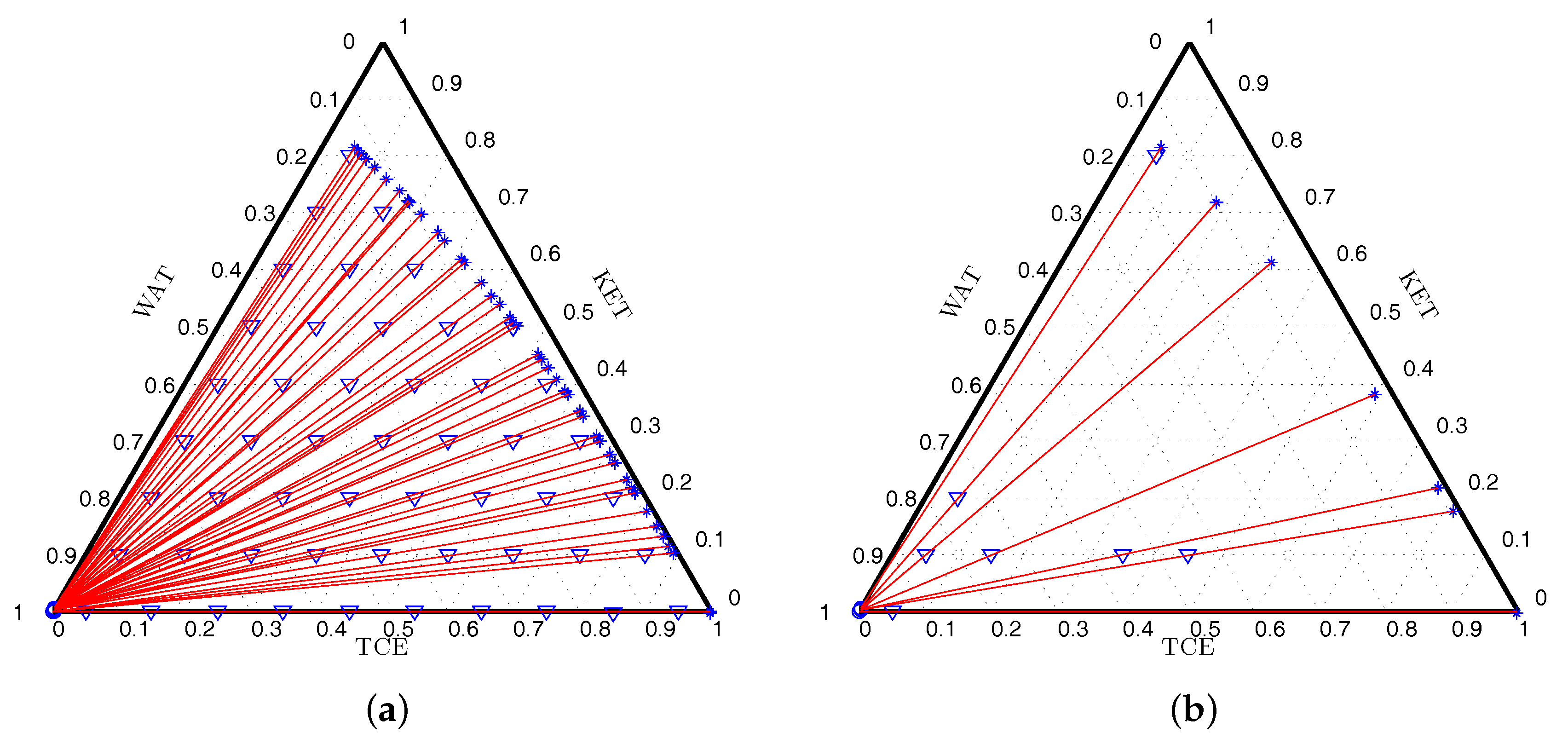
4.2. Example 2—Ternary System of Type 1, Class II; Including Dimensionless BIPs
Now, we consider ternary systems of Type 1 (Class II) and
only includes the dimensionless binary interaction parameters. The ternary system is formed by water (1), trichloroethylene (2) and acetone (3), represented by WAT-TCE–KET [
46]. The matrices
and
are:
The optimal designs obtained are listed in
Table 3 and the corresponding composition of the phases in equilibrium is in
Table 4. Here, we note the D-optimal design has seven support points, the A-optimality criterion produces a design with four points and the E-optimal design is formed by nine support points.
Figure 2a presents the initial set of candidate mixtures and corresponding tie-lines while
Figure 2b shows the tie-lines for the set of mixtures forming the D-optimal design (
Table 3).
4.3. Example 3—Ternary System of Type 1, Class I; Including Dimensionless and Non-Random BIPs
Here, we assume a ternary system of Type 1 (Class I) and
includes the dimensionless binary interaction parameters and the binary interaction non-randomness parameters. The support points of the optimal designs for this problem are shown in
Table 5; we note that the D-optimality criterion requires a design with 7 initial mixtures, A-optimality requires 9 and E-optimality needs 17, some of them having reduced relative importance (presented in two lines). Typically, all the designs have more support points than those in
Table 1, determined for the same system, when the aim was to estimate only the elements of matrix
. That the number of initial mixtures would increase was expected since the number of free parameters is larger. However, the computation time is similar to that of Example 1 as the number of candidate initial mixtures used is the same, which, in turn, yield SDP problems of equal size. The main difference is that the dimension of the FIM increases from six to nine.
Table 6 shows the equilibrium compositions for designs in
Table 5.


