Extremum Seeking Control for Discrete-Time with Quantized and Saturated Actuators

Abstract

This paper proposes an extremum-seeking controller (ESC) design for a class of discrete-time nonlinear control systems subject to input constraints or quantized inputs. The proposed method implements a proportional-integral ESC design along with a discrete-time anti-windup mechanism. The anti-windup enforces input saturation while preserving the input dither signal. The technique incorporates a mechanism for adjusting the amplitude of the extremum seeking control dither signal. This mechanism ensures that any violation of constraints due to the dither signal is removed while maintaining the probing signal active. An amplitude update routine is also proposed. The amplitude update is coupled with a saturation bias estimation algorithm that correctly accounts for the inherent bias associated with systems operated at or near saturation conditions. The amplitude update is designed to remove the dither signal when the system approaches the optimum. It also ensures that a lower bound of the amplitude is enforced to guarantee that excitation conditions are maintained.

1. Introduction

Extremum-seeking control (ESC) has grown to become the leading approach to solve real-time optimization problems [1]. Following the seminal work of Krstic and coworkers ([2,3,4,5,6,7]), this general and practically relevant control approach is equipped with an established and well understood theoretical framework, as highlighted in the proof of Krstic and Wang [2]. The standard perturbation ESC algorithm has been generalized in various forms to handle output and input constraints. ESC in the presence of constraints has been investigated in various form in the literature. Constrained ESC was first considered in [8] where a trajectory tracking approach was used to address the constrained ESC problem for a class of nonlinear systems with parametric uncertainties. In this approach, a barrier function or interior-point method was used to enforce constraints and feasibility of the closed-loop trajectories. A similar model-free extremum-seeking approach was presented in [9]. A Lagrangian, saddle-point, ESC technique is proposed in [10], and a similar approach is proposed in [11] to handle a class of stochastic control systems. In [12], a Shahshahani gradient approach was proposed. This techniques allows one to handle ESC problems subject to linear constraints by a simple reformulation of the gradient descent dynamics. In contrast to Lagrangian-based techniques, the main advantage of the Shahshahani gradient and barrier function approaches is the ability to preserve feasibility throughout the optimization.

For ESC in the presence of input constraints, a variety of techniques have been proposed. In [13] and [14], a projection algorithm is used to solve ESC problems subject to constraints in the decision variables. In [15], a comprehensive study of anti-windup mechanisms for standard ESC is presented. The approach draws a parallel between penalty (barrier) function methods and an anti-windup mechanism. A proof of convergence of the ESC in the presence of constraints is provided. In [16], a simplistic windup algorithm for a standard ESC technique is implemented experimentally for the real-time optimization of airside economizers.

The vast majority of existing results on ESC have focussed on continuous-time systems, as is the case for the existing approaches for ESC in the presence of constraints. Although discrete-time systems can be treated in an essentially similar fashion, the application of gradient descent in a discrete-time setting requires some care. A discrete-time version of the standard ESC loop was studied in [4,6] where convergence results similar to continuous time systems are obtained. A similar algorithm was also proposed in [17] for the tuning of PID controllers in unknown dynamical systems using ESC. Discrete-time ESC subject to stochastic perturbations is studied in [18]. The use of approximate parameterizations of the unknown cost function using quadratic functions was recently proposed in [19]. An alternative ESC-like method was proposed in [20]. In this study, a trajectory-based technique is used to analyze the properties of nonlinear optimization algorithms as dynamical systems. It is shown that properties of the nonlinear-optimization algorithms are suitable to assess the convergence of certain classes of ESC applied in a sampled-data approach. This method was recently studied in the context of global sampling methods in [21] where trajectory-based properties of nonlinear optimization methods are used to establish robust convergence. The main objective with the trajectory-based techniques is to analyze the properties of optimization algorithms assuming that they can converge to the true optimum using only the measurement of the objective function and possibly the constraints.

This paper proposes an extremum-seeking controller (ESC) design for a class of discrete-time nonlinear control systems subject to input constraints. Two actuation scenarios are considered. In the first scenario, we consider the ESC in the presence of saturated inputs. The proposed method generalizes the discrete-time proportional-integral ESC proposed in [22] to incorporate a new discrete-time anti-windup mechanism for ESC. One contribution of this study is the development of a saturation bias estimation mechanism that can be used to remove the impact of dither on or near the saturation level. This mechanism ensures that violation of the constraints due to the dither signal are removed without the introduction of a gradient estimation bias. Moreover, it allows the system to remain responsive to changes in the system despite operating on or very close to the saturation level. An amplitude update routine is also proposed as a discrete-time generalization of the method proposed in [23]. The amplitude update is coupled with the saturation bias estimation algorithm to account for the inherent bias associated with systems operated at or near saturation conditions.

In the second scenario, we adapt the application of the anti-reset windup strategy and the saturation bias estimation routine to handle systems with quantized actuators. We focus on ESC design for systems with “on/off” actuators. Since the excitation signal is limited to the on or off position, the application of the saturation bias estimation is able to remove the impact of the dither to allow the ESC system to converge to the correct position. Such actuators have not been treated in the literature.

The paper is organized as follows. A description of the ESC problem along with the key assumptions are given in Section 2. The proportional-integral ESC controller are presented in Section 3. The anti-windup mechanism and amplitude adjustment mechanism are described in Section 4. The design of ESC for quantized actuators are presented in Section 5. Simulation examples are presented in Section 6 followed by brief conclusions and proposed future work are in Section 7.

2. Problem Description

We consider a class of nonlinear systems of the form:

$$\begin{array}{ccc}\hfill x_{k+1}& =& x_k+f\left(x_k\right)+g\left(x_k\right)u_k\hfill \end{array}$$

(1)

$$\begin{array}{ccc}\hfill y_k& =& h\left(x_k\right)\hfill \end{array}$$

(2)

where $x_k\in {\mathbb{R}}^n$ is the vector of state variables at time k, $u_k$ is the input variable at time k taking values in $\mathcal{U}\subset \mathbb{R}$ and $y_k\in \mathbb{R}$ is the objective function at step k, to be minimized. It is assumed that $f\left(x_k\right)$ and $g\left(x_k\right)$ are smooth vector valued functions and that $h\left(x_k\right)$ is a unknown smooth function.

The objective is to stabilize the system at the equilibrium conditions, $x^{*}$ and $u^{*}$, that achieves the minimum value of $y(=h\left(x^{*}\right))$ subject to saturation of the input. The input variable, $u_k$, is required to lie in the interval $\mathcal{U}=[u_{-},u_{+}]$. At equilibrium, the state variables are given by the map $x=\pi \left(u\right)$ that solves the following equation:

$$\begin{array}{c}\hfill f\left(\pi \right(u\left)\right)+g\left(\pi \right(u\left)\right)u=0.\end{array}$$

The corresponding equilibrium cost function is given by:

$$\begin{array}{c}\hfill y=h\left(\pi \right(u\left)\right)=\ell \left(u\right)\end{array}$$

(3)

The steady-state optimization problem is to find the minimizer $u^{*}$ of $y=\ell \left(u^{*}\right)$ subject to $u^{*}\in \mathcal{U}$. The set $\mathcal{D}\left(u\right)$ represents a neighbourhood of the equilibrium $x=\pi \left(u\right)$.

The steady-state cost function, $\ell \left(u\right)$, meets the following assumptions.

Assumption 1.

The nonlinear system is such that

$$\begin{array}{c}\hfill {\nabla }_{x}h\left(\pi \left(u\right)\right)g\left(\pi \left(u\right)\right)(u-u^{*})\ge 0\end{array}$$

$\forall u\in \mathcal{U}$.

Assumption 2.

The cost $h\left(x\right)$ is such that

• $\frac{\partial h\left(x^{*}\right)}{\partial x}=0$
• $\frac{{\partial }^{2}h\left(x\right)}{\partial x\partial x^T}>\beta I,\forall x\in {\mathbb{R}}^n$

where β is a strictly positive constant.

Following [22], we write the cost dynamics as:

$$\begin{array}{c}\hfill y_{k+1}-y_k={\Psi }_{0,k}(x_k,{\widehat{u}}_k)+{\Psi }_{1,k}(x_k,u_k,{\widehat{u}}_k)(u_k-{\widehat{u}}_k).\end{array}$$

(4)

where ${\Psi }_{0,k}(x_k,{\widehat{u}}_k)=h\left(\alpha (x_k,{\widehat{u}}_k)\right)-h\left(x_k\right)$,

$$\begin{array}{c}\hfill {\Psi }_{1,k}(x_k,u_k,{\widehat{u}}_k)=(\nabla h\left(\alpha \left(x_k\right)\right)g\left(x_k\right)+\frac{1}{2}{(u_k-{\widehat{u}}_k)}^{\top }g{\left(x_k\right)}^{\top }{\nabla }^{2}h\left({\tilde{y}}_k\right)g\left(x_k\right).\end{array}$$

and ${\overline{y}}_k=\alpha \left(x_k\right)+\theta g\left(x_k\right)(u_k-{\widehat{u}}_k)$ for $\theta \in (0,1)$.

The following assumptions are required to ensure the stability of the closed-loop system.

Assumption 3.

There exists a function $u_k={\alpha }_F(x_k,{\widehat{u}}_k)$ that solves the identity:

$$\begin{array}{c}\hfill {\alpha }_F(x_k,{\widehat{u}}_k)=\mathrm{Sat}(-k_g{\Psi }_{1,k}(x_k,{\alpha }_F(x_k,{\widehat{u}}_k),{\widehat{u}}_k)+{\widehat{u}}_k).\end{array}$$

This assumption states that the feedback:

$$\begin{array}{c}\hfill u_k=\mathrm{Sat}(-k_g{\Psi }_{1,k}(x_k,u_k,{\widehat{u}}_k)+{\widehat{u}}_k).\end{array}$$

is well defined.

The following stabilizability condition for the nonlinear system subject to input saturation is also required.

Assumption 4.

There exists a positive definite function $\left(x\right)$ that satisfies the following inequalities:

$$\begin{array}{c}\hfill {\beta }_1\parallel x-\pi \left(\widehat{u}\right){\parallel }^2\le \mathcal{V}\left(x\right)\le {\beta }_2{\parallel x-\pi \left(\widehat{u}\right)\parallel }^2\end{array}$$

with positive constants ${\beta }_1$ and ${\beta }_2$. For all $x\in {\Omega }_{\beta }=\left\{x\in {\mathbb{R}}^n\left|\mathcal{V}\left(x\right)\le \beta \right.\right\}\subset \mathcal{D}\left(\widehat{u}\right)$ there exists a positive constant $k_g^{*}$ such that:

$$\begin{array}{c}\hfill \mathcal{V}\left(\overline{\alpha }\left(x_k\right)\right)-\mathcal{V}\left(x_k\right)\le -{\alpha }_e{\parallel x_k-\pi \left(\widehat{u}\right)\parallel }^2\end{array}$$

with positive constant ${\alpha }_e$ and $\forall \widehat{u}\in \mathcal{U}$ and

$$\overline{\alpha }\left(x_k\right)=x_k+f\left(x_k\right)-k_g^{*}g\left(x_k\right){\Psi }_{1,k}(x_k,{\alpha }_F,\widehat{u})+g\left(x_k\right)\widehat{u}.$$

3. Proportional-Integral Discrete-Time ESC

In this section, we present the basic PI-ESC controller and the proposed parameter (gradient) estimation algorithm.

PI-ESC Controller

From (4), the objective function dynamics are parameterized as follows:

$$\begin{array}{c}\hfill y_{k+1}=y_k+{\theta }_{0,k}+{\theta }_{1,k}^T(u_k-{\widehat{u}}_k)\end{array}$$

where the time-varying parameters ${\theta }_{0,k}$ and ${\theta }_{1,k}$ are identified with ${\theta }_{0,k}={\Psi }_{0,k}$ and ${\theta }_{1,k}={\Psi }_{1,k}^T$.

The unknown parameters ${\theta }_{0,k}$ and ${\theta }_{1,k}$ must be estimated using a parameter estimation approach described in the next subsection. We let ${\widehat{\theta }}_{0,k}$ and ${\widehat{\theta }}_{1,k}$ denote the estimates of ${\theta }_{0,k}$ and ${\theta }_{1,k}$, respectively. The proportional-integral extremum-seeking controller is given by:

$$\begin{array}{cc}\hfill u_k& =\mathrm{Sat}\left(-k_g{\widehat{\theta }}_{1,k}+{\widehat{u}}_k+d_k\right)\hfill \\ \hfill {\widehat{u}}_{k+1}& ={\widehat{u}}_k-\frac{k_g}{{\tau }_I}{\widehat{\theta }}_{1,k},\hfill \end{array}$$

(5)

where $k_g$ and ${\tau }_I$ are positive constants to be assigned. The term $d_k$ is a dither signal used to provide a sufficiently excited signal in closed-loop. The dither signal is bounded such that $\parallel d_k\parallel \le D$ where D a known positive constant denotes the amplitude of the dither.

In this study, the estimation of the parameter varying parameters ${\theta }_{0,k}$ and ${\theta }_{1,k}$ is performed using the estimation routine described in [22]. The estimation routine implements a modified recursive least squares approach for the estimation of time-varying parameters. It is described briefly in Appendix A.

The stability properties of the ESC considered are summarized in Appendix B.

4. Input Constrained ESC

In this section, we present the main contribution of this study. The proposed technique incorporates three mechanisms for the solution of ESC problems in the presence of input constraints. The first mechanism consists of a standard anti-windup mechanism that exploits the proportional integral formulation of the ESC considered. The second mechanism proposes a dither bias estimation routine that eliminates the presence of biases introduced when the dither signal input pushes the input to its saturation limit. The third mechanism is a dither amplitude update that is used to remove the dither signal when the system has converged to its optimal value, or its optimal saturation limit.

4.1. Anti-Windup Mechanism

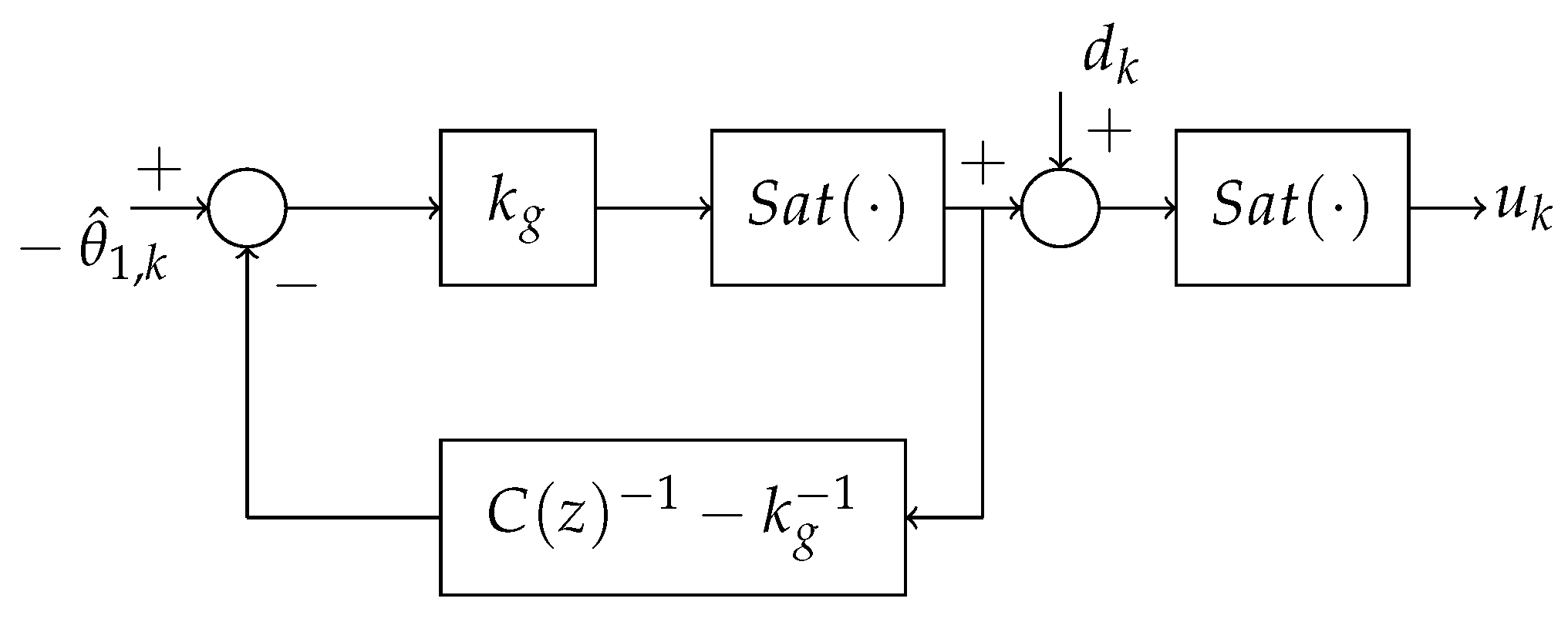
In this paper, we propose the use of an anti-windup mechanism for the proportional integral ESC controller (5). A block diagram of the mechanism is shown in Figure 1.

In Figure 1, $C\left(z\right)$ represents the discrete-time transfer function of the proportional-integral controller

$$C\left(z\right)=k_g+\frac{k_g}{{\tau }_I}\frac{1}{z-1}.$$

The mechanism places the dither addition after the anti-windup loop but before the final saturation. This mechanism guarantees that the dither signal is not removed when the system operates at the saturation limits. It also guarantees that the dithered input does not violate the input constraints.

The operator Sat$(·)$ denotes the saturation function:

$$\begin{array}{c}\hfill \mathrm{Sat}\left(u\right)=\left\{\begin{array}{cc}{u}_{-}\hfill & ifu\le u_{-},\hfill \\ u\hfill & if{u}_{-}<u\le u_{+},\hfill \\ u_{+}\hfill & ifu\ge u_{+}.\hfill \end{array}\right.\end{array}$$

(6)

The proposed dynamics of the anti-windup mechanism is given by:

$$\begin{array}{cc}\hfill z_{k+1}& =z_k-\frac{1}{{\tau }_I}{z}_k-\frac{1}{k_g{\tau }_I}\mathrm{Sat}(-k_g{\widehat{\theta }}_{1,k}-k_g{z}_k)\hfill \\ \hfill u_k& =\mathrm{Sat}(\mathrm{Sat}(-k_g{\widehat{\theta }}_{1,k}-k_g{z}_k)+d_k).\hfill \end{array}$$

(7)

The anti windup loop is such that, in the absence of saturation, the control law reduces to the proportional integral law and the control law becomes:

$$\begin{array}{cc}\hfill u_k& =\mathrm{Sat}(-k_g{\widehat{\theta }}_{1,k}-k_g{\widehat{z}}_k+d_k)\hfill \\ \hfill {\widehat{z}}_{k+1}& ={\widehat{z}}_k+\frac{1}{{\tau }_I}{\widehat{\theta }}_{1,k}.\hfill \end{array}$$

(8)

Please note that the Sat$(·)$ remains in the control loop to ensure that the added dither signal does not cause input constraint violation.

One of the difficulties associated with such an approach is that the saturation creates a bias in the dither signal. This is problematic in cases where the optimum input lies close to or on the saturation limit. This bias in the dither signal can lead to a bias in the estimation of the parameters. As result, the value of the parameter ${\widehat{\theta }}_{1,k}$ does not converge to zero even when the true value ${\theta }_{1,k}$ vanishes.

It is, therefore, imperative to provide a mechanism to introduce the dither signal that prevents the estimation bias. We consider two mechanisms in this study.

4.2. Saturation Bias Estimation

Let us consider the case in which the optimum occurs on the upper saturation level $\overline{u}$. At the optimum, the control signal for the ESC is given by

$$u=\mathrm{Sat}(\overline{u}+d_k).$$

The filter (or regressor) vector yields:

$$w_{k+1}^T=w_k^T-K{w}_k^T+\left[1,\mathrm{Sat}(\overline{u}+d_k)\right]$$

One of the key properties of the dither signal is that $\frac{1}{N}{\sum }_{i=k}^{k+N-1}{d}_i=0$. In the absence of input saturation, the average regressor is such that

$$\underset{k\to \infty }{lim}\frac{1}{N}\sum _{i=k}^{k+N-1}{w}_i=\frac{1}{K}{[1,\overline{u}]}^T.$$

In the presence of a bias in the dither signal, the regressor vector does not average to the correct value. As a result, the parameter estimation of ${\theta }_{1,k}$ is subject to a bias, and the system would converge to an erroneous optimum state and input.

In this section, we design an update mechanism that accounts for this saturation bias. This is achieve by introducing a signal ${\delta }_k$ in the control, $u_k$, which is such that the average input is unbiased. That is, for a fixed value of the input $u_k=\overline{u}$, the following property is achieved:

$$\begin{array}{c}\hfill \frac{1}{N}\sum _{i=k}^{k+N-1}\mathrm{Sat}(\overline{u}+d_i+{\delta }_k)=\overline{u}.\end{array}$$

(9)

We first define the variable

$$\begin{array}{cc}\hfill {{\rm Y}}_k=(\mathrm{Sat}\left(\mathrm{Sat}\right(-k_g{\widehat{\theta }}_{1,k}& -k_g{\widehat{z}}_k)+d_k+{\delta }_k)-\mathrm{Sat}(-k_g{\widehat{\theta }}_{1,k}-k_g{\widehat{z}}_k)).\hfill \end{array}$$

The bias estimation update proposed in this study is given by:

$$\begin{array}{c}\hfill {\delta }_{k+1}={\delta }_k-\left\{\begin{array}{cc}\lambda {{\rm Y}}_k\hfill & \mathrm{if}{u}_k=u_{-}\mathrm{or}{u}_k=u_{+}\hfill \\ \lambda {\delta }_k\hfill & \mathrm{otherwise}\hfill \end{array}\right.\end{array}$$

(10)

Proposition 1.

The saturation bias estimate update (10) is such that:

• For $u_k\in (u^{-},u^{+})$,

  $$\underset{k\to \infty }{lim}{\delta }_k=0$$
• For $u=u^{-}$, or $u=u^{+}$,

  $$\underset{k\to \infty }{lim}\sum _{i=k}^{k+N-1}\mathrm{Sat}(u+d_i+{\delta }_k)=u.$$

Proof. 

For Statement 1, the conclusion is straightforward.

The proof of Statement 2 is as follows. To establish the property (9), we first compute the average in the case where the value of the input is at one its saturation limits. Let us consider the case where the input is at its upper limit, $u_{+}$. From a set of N samples of the input, assume that there are $N_1$ samples at which Sat$(u_{+}+d_k+{\delta }_k)=u_{+}$ with the remaining $N_2$ samples for which Sat$(u_{+}+d_k+{\delta }_k)<u_{+}$. Let ${\mu }_2\left(j\right)$, $j=1,\dots ,N_2$ denote the indices of the samples that are not saturated. As a result, we can decompose the averaged quantity as follows:

$$\begin{array}{cc}\hfill \sum _{i=k}^{k+N-1}\mathrm{Sat}(u_{+}+d_i+{\delta }_i)& =u_{+}+\sum _{j=1}^{N_2}(d_{{\mu }_2\left(j\right)}+{\delta }_{{\mu }_2\left(j\right)})=u_{+}+\sum _{j=1}^{N_2}{d}_{{\mu }_2\left(j\right)}+\sum _{j=1}^{N_2}{\delta }_{{\mu }_2\left(j\right)}.\hfill \end{array}$$

Thus if one considers the update (10). Following the above argument, we average both sides by summing over N samples. Let us consider the situation where the input is at its upper saturation limit $u_{+}$ and decompose the overall average into $N_1$ saturated values and $N_2$ inputs whose perturbed value is not saturated. This yields

$$\begin{array}{cc}\hfill \sum _{i=k}^{k+N-1}{\delta }_{i+1}=\sum _{i=k}^{k+N-1}{\delta }_i& -\lambda \sum _{j=1}^{N_1}\left(\mathrm{Sat}(u_{+}+d_{{\mu }_1\left(j\right)}+{\delta }_{{\mu }_1\left(j\right)})-\mathrm{Sat}\left(u_{+}\right)\right)\hfill \\ & -\lambda \sum _{j=1}^{N_2}\left(\mathrm{Sat}(u_{+}+d_{{\mu }_2\left(j\right)}+{\delta }_{{\mu }_2\left(j\right)})-\mathrm{Sat}\left(u_{+}\right)\right)\hfill \end{array}$$

This gives the following recursion of sums:

$$\begin{array}{cc}\hfill \sum _{i=k}^{k+N-1}& {\delta }_{i+1}=\sum _{i=k}^{k+N-1}{\delta }_i-\lambda \sum _{j=1}^{N_2}{d}_{{\mu }_2\left(j\right)}-\lambda \sum _{j=1}^{N_2}{\delta }_{{\mu }_2\left(j\right)}.\hfill \end{array}$$

For every sample from the set of points that are saturated at step k, it follows that ${\delta }_{{\mu }_1\left(j\right)+1}={\delta }_{{\mu }_1\left(j\right)}$. As a result, we can write

$$\begin{array}{c}\hfill \sum _{j=1}^{N_2}{\delta }_{{\mu }_2\left(j\right)+1}=\sum _{i=1}^{N_2}{\delta }_{{\mu }_2\left(j\right)}-\lambda \sum _{j=1}^{N_2}{d}_{{\mu }_2\left(j\right)}-\lambda \sum _{j=1}^{N_2}{\delta }_{{\mu }_2\left(j\right)}.\end{array}$$

Defining the variable

$${\overline{\delta }}_k=\sum _{j=1}^{N_2}{\delta }_{{\mu }_2\left(j\right)},$$

we obtain the following recursion:

$${\overline{\delta }}_{k+1}={\overline{\delta }}_k-\lambda {\overline{\delta }}_k-\lambda {\overline{d}}_k.$$

As a result, we see that the average ${\overline{\delta }}_k$ approaches the negative value of the mean dither ${\overline{d}}_k$. As a result, the bias (9) is completely removed by the saturation bias update (10). This completes the proof of Statement 2. □

In cases where the optimum lies on or close to a saturation, the update (10) would lead to an effective removal of the dither signal. However, in fact, the dither is not removed. It is simply compensated for by the bias estimate ${\delta }_k$. If a disturbances affects the system, moving the optimum inside the saturation, then the dither signal would resume and the ESC would operate in a normal way. As a result, the dither would not be effectively removed.

4.3. Dither Amplitude Update

In this study, we consider a dither signal of the form: $d_k=a_{k}sin\left({\nu }_k\right)$ where ${\nu }_k$ can be taken to be a zero-mean Gaussian variable or simply ${\nu }_k=\omega k$ for some frequency $\omega$. The amplitude of the dither signal $a_k$ is obtained using an amplitude update.

Let the upper or lower limit if $u_k$ be denoted generically by $\overline{u}$. We first define the signal:

$$\begin{array}{c}\hfill {\Theta }_k=\left\{\begin{array}{cc}{\widehat{\theta }}_{1,k}\hfill & u_k\ne \overline{u},\hfill \\ {\widehat{\theta }}_{0,k}+{\widehat{\theta }}_{1,k}\overline{u}\hfill & \mathrm{otherwise}.\hfill \end{array}\right.\end{array}$$

The proposed amplitude update is given by:

$$\begin{array}{c}\hfill \begin{array}{c}\hfill a_{k+1}=a_k+{\sigma }_1\left({\gamma }_1\frac{2}{\pi }{tan}^{-1}\left({\Theta }_k\right)-{\gamma }_2{\lambda }_{min}\left[{\Sigma }_k\right]-a_k\right)\end{array}\end{array}$$

(11)

where $a_0\ge 0$, ${\sigma }_1$, ${\gamma }_1$ and ${\gamma }_2$ are tuning parameters. This mechanism confers two actions to adjust the amplitude of the dither signal.

The term ${\gamma }_1\frac{2}{\pi }{tan}^{-1}\left({\Theta }_k\right)$ decreases the amplitude when the gradient estimate decreases or when the system has reached an equilibrium corresponding to a saturation input level. In [23], a similar amplitude update is proposed. The proposed method complements that approach in two ways. First, we adjust for the situation in which the input has stabilized on a saturation level. In this case, the estimated value of ${\theta }_{1,k}$ cannot reach 0. As a result, the approach of [23] using only ${\widehat{\theta }}_{1,k}$ would yield a larger value of the amplitude. If the optimization does not lead to a saturated value of the input, the update acts as the update of [23] and reduces the amplitude to a suitable lower level.

Second, the proposed method assigns a minimum value of the amplitude $a_k$. As the proof of stability of the PI-ESC algorithm demonstrates [22], the practical stability of the unknown optimum requires a persistent dither signal with $a_k>0$ for all k. In practice, setting $a_k=0$ would prevent the system from responding to possible changes in the changes that may arise from changing conditions. This property of the ESC system was recognized in [23], which required a fixed lower bound for the amplitude. However, the choice of this lower bound can be conservative. The second term in the update (11), ${\gamma }_2{\lambda }_{min}\left[{\Sigma }_k\right]$, aims to increase the amplitude $a_k$ when the smallest eigenvalue of the matrix $\Sigma$ decreases. This update guarantees a minimum amount of excitation in the system in order to respond to possible process changes.

The action of the amplitude update can be summarized as follows.

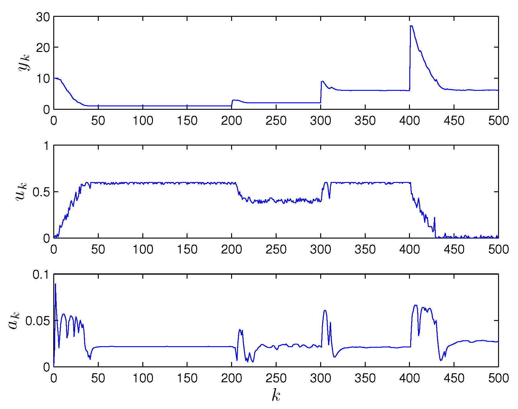
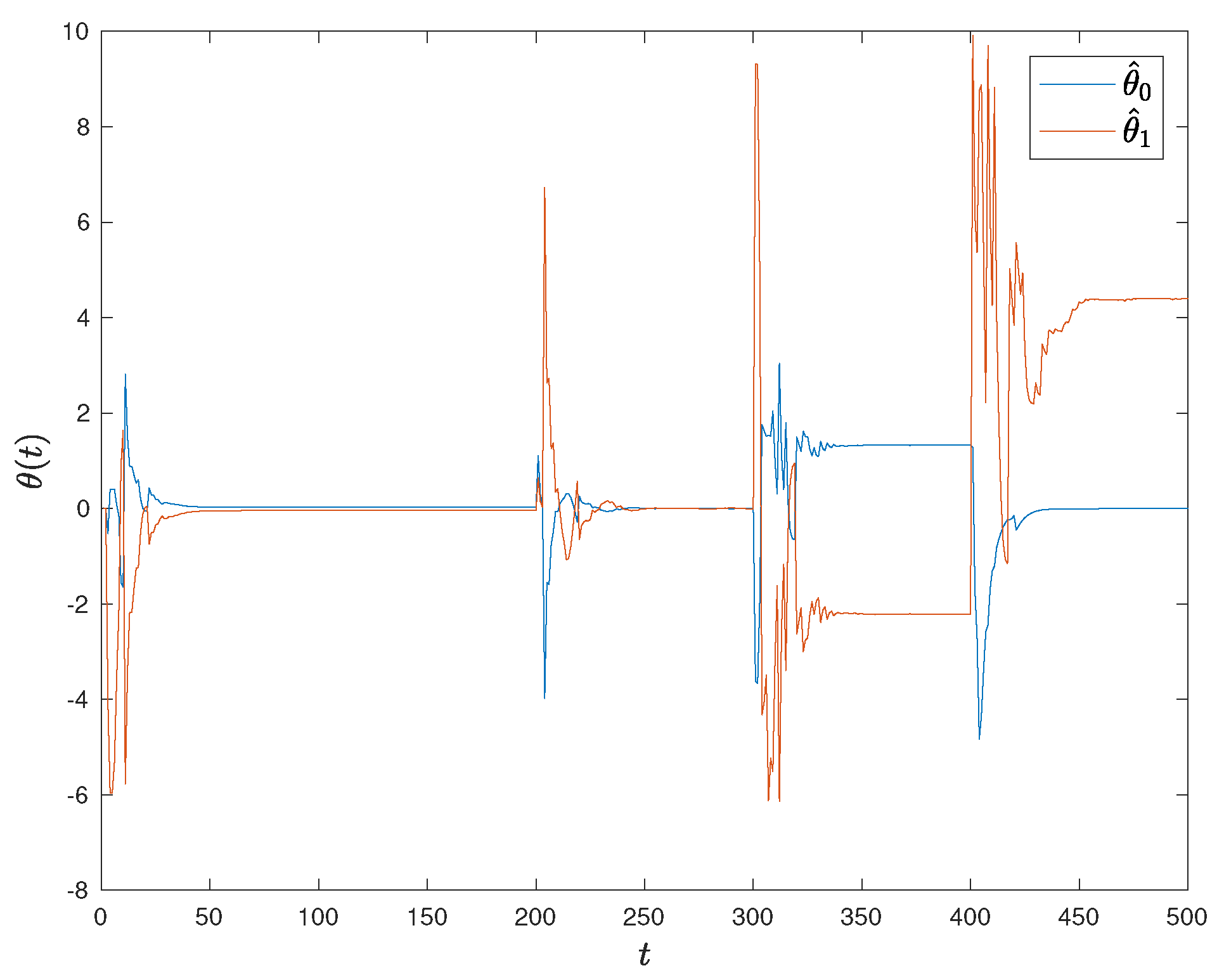
Proposition 2.

For ${\sigma }_1<1$, the update (11) is such that $a_k$ is bounded and ${lim}_{k\to \infty }{a}_k$ approaches ${\gamma }_2{\lambda }_{min}\left[{\Sigma }_{\infty }\right]$ in a region of an unconstrained optimum ${\widehat{\theta }}_{1,k}=0$ or on a saturation level of the input ${\widehat{\theta }}_{0,k}+{\widehat{\theta }}_{1,k}\overline{u}=0$.

The combination of the anti-windup (Figure 1) and the amplitude update (11) provides an effective mechanism to minimize the bias of the system arising from the saturation. It also removes the need for the tuning of the amplitude. We demonstrate this in simulations in the next section.

5. ESC for Systems with Quantized Actuators

The three mechanisms proposed in the previous section can be easily adapted to a situation where the actuators of the system are limited to quantized (or on-off) input settings. In this case, we consider an actuator whose on-off action can be implemented using a hysteresis mechanism of the form:

$$\begin{array}{c}\hfill u=\Gamma (u,ϵ)=\left\{\begin{array}{cc}{u}_{-}\hfill & \mathrm{if}u\le (u_{-}+u_{+})/2+ϵ\hfill \\ u_{+}\hfill & \mathrm{if}u\ge (u_{-}+u_{+})/2-ϵ\hfill \end{array}\right.\end{array}$$

(12)

where $ϵ>0$ is a small positive constant. The function $\Gamma \left(u\right)$ implements the discrete actuator using a hysteresis mechanism.

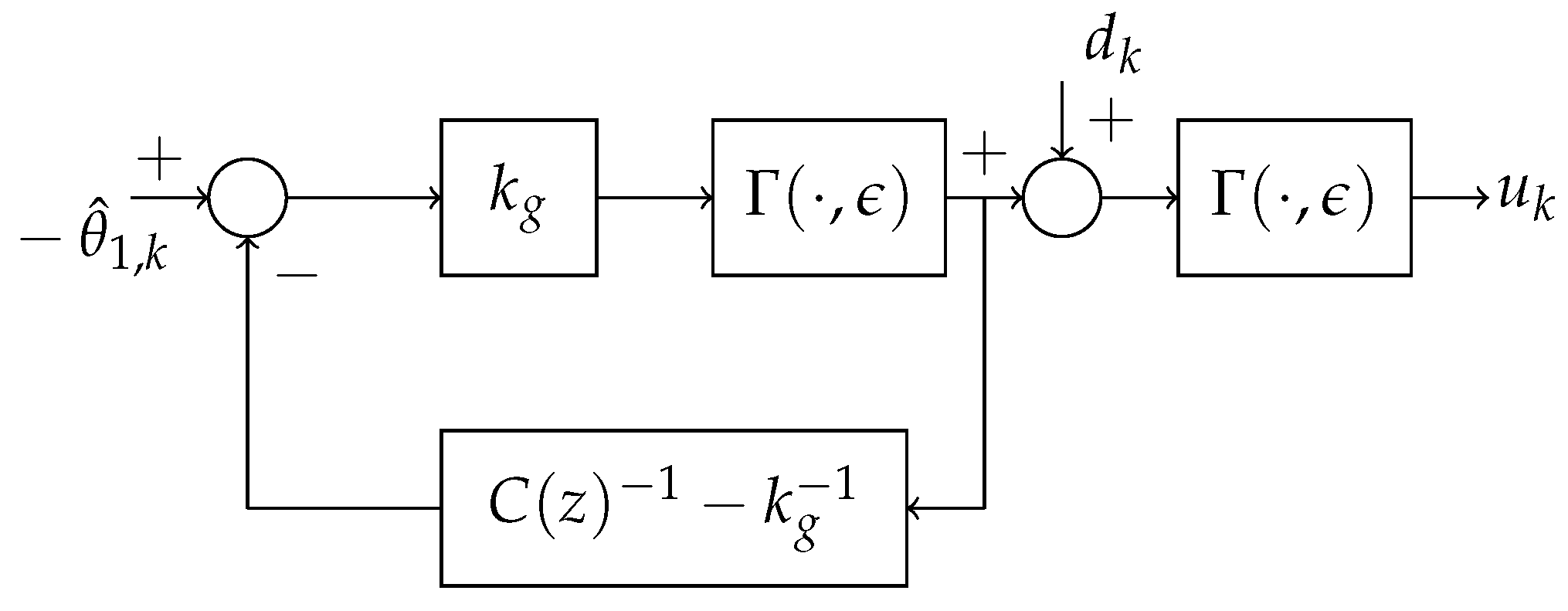
In this study, we propose a quantized actuator ESC using the mechanism depicted in Figure 2.

As above, we consider the anti-windup ESC given by:

$$\begin{array}{cc}\hfill u_k& =\Gamma (-k_g{\widehat{\theta }}_{1,k}-k_g{\widehat{z}}_k+d_k,ϵ)\hfill \\ \hfill {\widehat{z}}_{k+1}& ={\widehat{z}}_k+\frac{1}{{\tau }_I}{\widehat{\theta }}_{1,k}.\hfill \end{array}$$

(13)

Since the ESC only provides quantized control action $u_k=u_{+}$ or $u_k=u_{-}$, we must consider a saturation bias estimation to eliminate the bias and remove the b presented in Section 4.3. The reason for this is that the update (14) yields the required property of the saturation bias as the system reaches the limits. The proposed bias update is given by:

$$\begin{array}{c}\hfill {\delta }_{k+1}={\delta }_k-\left\{\begin{array}{cc}\lambda {{\rm Y}}_k\hfill & \mathrm{if}{u}_k=u_{-}\mathrm{or}{u}_k=u_{+}\hfill \\ \lambda {\delta }_k\hfill & \mathrm{otherwise}\hfill \end{array}\right.\end{array}$$

(14)

where

$$\begin{array}{cc}\hfill {{\rm Y}}_k=\Gamma (\Gamma (-k_g{\widehat{\theta }}_{1,k}& -k_g{\widehat{z}}_k)+d_k+{\delta }_k,ϵ)-\Gamma (-k_g{\widehat{\theta }}_{1,k}-k_g{\widehat{z}}_k,ϵ).\hfill \end{array}$$

The amplitude of the dither signal is implemented as in Section 4.3.

6. Simulation

6.1. Anti-Windup PIESC

We consider the application of the PI-ESC approach to the following linear discrete-time system:

$$\begin{array}{c}\hfill \begin{array}{cc}\hfill x_{k+1}& =a_1{x}_k+u_k\hfill \\ \hfill y_k& ={(x_k-p_1)}^2+q_1\hfill \end{array}\end{array}$$

where $a_1=0.8$,

$$\begin{array}{c}\hfill p_1=\left\{\begin{array}{cc}3\hfill & k<200\hfill \\ 2\hfill & 200\le k<300\hfill \\ 4\hfill & 300\le k<400\hfill \\ -2\hfill & k\ge 400\hfill \end{array}\right.,q_1=\left\{\begin{array}{cc}1\hfill & k<200\hfill \\ 2\hfill & 200\le k<300\hfill \\ 5\hfill & 300\le k<400\hfill \\ 2\hfill & k\ge 400\hfill \end{array}\right..\end{array}$$

The input variable $u_k$ in constrained to values over the interval $[0,0.6]$.

We consider the PIESC algorithm with $k=0.1$ and ${\tau }_I=5$. The estimation routine parameters are set to $\alpha =0.25$, $\sigma ={10}^{-5}$ and $K_k=0.99$. The amplitude is used with ${\gamma }_1=0.1$, ${\gamma }_2=0.01$ and ${\sigma }_1=0.1$ with an initial condition $a_0=0$. The dither signal is $d_k=a_{k}sin\left(2k\right).$ The choice of these tuning parameters reflect the tuning guidelines that have been presented in [22]. For the saturation bias update is implemented with $\lambda =0.05$. This choice guarantees that the bias update responds quickly to changing conditions.

The simulation results are shown in Figure 3 and Figure 4. Figure 3 shows the input and output trajectories for the resulting closed-loop system. It also shows the changes in the amplitude of the dither signal. Figure 4 shows the corresponding parameter estimates.

In this simulation, the location of the optimum is changed. For $k\in [0,200]$, the optimum occurs at $y^{*}=1$ with $u^{*}=0.6$. This places the minimizer directly on the input constraint. The ESC system identifies the optimum correctly. The amplitude update rule is also able to reduce the amplitude to a suitable minimum level. For $k\in [200,300]$, the unknown optimum occurs at $y^{*}=2$ and $u^{*}=0.4$. Since the dither amplitude update routine (11) prevented the amplitude from values that are too small, the PIESC is able to respond quickly to the change in conditions.

For the period $k\in [300,400]$, the unconstrained minimum occurs at $y^{*}=5$ and $u^{*}=0.8$. As required in this case, the PIESC system converges to the saturated value of $u_k=0.6$ with cost $y_k=6$. Finally, for $k\ge 400$, the system cannot reach the unconstrained optimum $y^{*}=2$ and $u^{*}=-0.4$ but converges correctly to the lower saturation level of $u_k=0$ with cost $y_k=6$.

Overall, the PIESC with anti-windup mechanism performs effectively. First, the system is able to perform the optimization task in the presence of input saturation. Second, the proposed approach allows the partial removal of the dither signal when the system operates at saturation.

6.2. Quantized Actuator ESC

In this section, we consider the same dynamical system subject to the quantized actuator:

$$\begin{array}{c}\hfill \Gamma (u,ϵ)=\left\{\begin{array}{cc}0\hfill & \mathrm{if}u\le 0.3+ϵ\hfill \\ 0.6\hfill & \mathrm{if}u\ge 0.3-ϵ\hfill \end{array}\right.\end{array}$$

(15)

where $ϵ=0.01$ for the purpose of simulation.

The proposed dither signal is given by the sine wave signal:

$$\begin{array}{c}\hfill d_k=a_k\mathrm{sign}(sin\left(\omega k\right))+{\delta }_k\end{array}$$

(16)

where ${\delta }_k$ is the bias update and $\mathrm{sign}(·)$ is the sign function.

The parameters, $p_1$ and $q_1$, are chosen as follows:

$$\begin{array}{c}\hfill p_1=\left\{\begin{array}{cc}3\hfill & k<200\hfill \\ -1\hfill & 200\le k<300\hfill \\ 4\hfill & 300\le k<400\hfill \\ -2\hfill & k\ge 400\hfill \end{array}\right.,q_1=\left\{\begin{array}{cc}1\hfill & k<200\hfill \\ 2\hfill & 200\le k<300\hfill \\ 5\hfill & 300\le k<400\hfill \\ 2\hfill & k\ge 400\hfill \end{array}\right..\end{array}$$

We consider the PIESC algorithm with $k=0.1$ and ${\tau }_I=5$. The estimation routine parameters are set to $\alpha =0.25$, $\sigma ={10}^{-5}$ and $K_k=0.99$. The amplitude is used with ${\gamma }_1=0.1$, ${\gamma }_2=0.01$ and ${\sigma }_1=0.9$ with an initial condition $a_0=0.5$. We consider the bias update (14) with update parameter $\lambda =0.95$.

The simulation results are shown in Figure 5. The ESC system is able to respond quickly to the changing conditions. The correct optimal setting of the discrete actuator is correctly identified, $u^{*}=0.6$ for $0\le t\le 200$, $u^{*}=0$ for $200<t\le 300$, $u^{*}=0.6$ for $300<t\le 400$ and $u^{*}=0$ for $t\ge 400$. The combination of the amplitude update and the bias estimation works very effectively in this case. The systems reintroduces excitation in the system in response to the change in conditions. The resulting excitation introduces a short sequence of discrete switches that vanish once the correct optimum is identified.

7. Conclusions

This study proposed an extremum-seeking control algorithm for systems subject to input saturated or quantized actuators. The approach couples a well known anti-reset windup technique with a saturation bias estimation routine that improves the performance of the ESC near or on the saturation level by removing the impact of the dither signal. An amplitude update is also proposed to further improve the performance of the ESC system.

References

1. Tan, Y.; Moase, W.; Manzie, C.; Nesic, D.; Mareels, I. Extremum seeking from 1922 to 2010. In Proceedings of the 29th Chinese Control Conference (CCC), Beijing, China, 29–31 July 2010; pp. 14–26. [Google Scholar]
2. Krstic, M.; Wang, H. Stability of Extremum Seeking Feedback for General Dynamic Systems. Automatica 2000, 36, 595–601. [Google Scholar] [CrossRef]
3. Krstic, M. Performance Improvement and Limitation in Extremum Seeking Control. Syst. Control Lett. 2000, 39, 313–326. [Google Scholar] [CrossRef]
4. Ariyur, K.B.; Krstic, M. Real-Time Optimization by Extremum-Seeking Control; John Wiley and Sons Inc.: Hoboken, NJ, USA, 2003. [Google Scholar]
5. Ariyur, K.; Krstic, M. Analysis and design of multivariable extremum seeking. In Proceedings of the American Control Conference, Anchorage, AK, USA, 8–10 May 2002; pp. 2903–2908. [Google Scholar]
6. Choi, J.Y.; Krstic, M.; Ariyur, K.; Lee, J. Extremum seeking control for discrete-time systems. IEEE Trans. Autom. Control 2002, 47, 318–323. [Google Scholar] [CrossRef]
7. Wang, H.; Krstic, M.; Bastin, G. Optimizing Bioreactors by Extremum Seeking. Int. J. Adapt. Control Signal Process. 1999, 13, 651–669. [Google Scholar] [CrossRef]
8. DeHaan, D.; Guay, M. Extremum-seeking control of state-constrained nonlinear systems. Automatica 2005, 41, 1567–1574. [Google Scholar] [CrossRef]
9. Guay, M.; Moshksar, E.; Dochain, D. A constrained extremum-seeking control approach. Int. J. Robust Nonlinear Control 2015, 25, 3132–3153. [Google Scholar] [CrossRef]
10. Durr, H.B.; Zeng, C.; Ebenbauer, C. Saddle Point Seeking for Convex Optimization Problems. In Proceedings of the IFAC Symposium on Nonlinear Control Systems, Toulouse, France, 4–6 September 2013; pp. 540–545. [Google Scholar]
11. Coito, F.; Lemos, J.; Alves, S. Stochastic Extremum Seeking in the Presence of Constraints. In Proceedings of the IFAC World Congress, Prague, Czech Republic, 3–8 July 2005; Volume 16, pp. 266–271. [Google Scholar]
12. Poveda, J.; Quijano, N. A Shahshahani Gradient based extremum seeking scheme. In Proceedings of the 2012 IEEE 51st Annual CDC, Maui, HI, USA, 10–13 December 2012; pp. 5104–5109. [Google Scholar] [CrossRef]
13. Mills, G.; Krstic, M. Constrained extremum seeking in 1 dimension. In Proceedings of the 53rd IEEE Conference on Decision and Control, Los Angeles, CA, USA, 15–17 December 2014; pp. 2654–2659. [Google Scholar] [CrossRef]
14. Mills, G.; Krstic, M. Gradient based projection method for constrained optimization. In Proceedings of the 52nd IEEE Conference on Decision and Control, Florence, Italy, 10–13 December 2013; pp. 2966–2971. [Google Scholar] [CrossRef]
15. Tan, Y.; Li, Y.; Mareels, I.M.Y. Extremum Seeking for Constrained Inputs. IEEE Trans. Autom. Control 2013, 58, 2405–2410. [Google Scholar] [CrossRef]
16. Mu, B.; Li, Y.; House, J.M.; Salsbury, T.I. Experimental evaluation of anti-windup extremum seeking control for airside economizers. Control Eng. Pract. 2016, 50, 37–47. [Google Scholar] [CrossRef]
17. Killingsworth, N.J.; Krstic, M. PID tuning using extremum seeking: Online, model-free performance optimization. IEEE Control Syst. Mag. 2006, 26, 70–79. [Google Scholar]
18. Manzie, C.; Krstic, M. Extremum seeking with stochastic perturbations. IEEE Trans. Autom. Control 2009, 54, 580–585. [Google Scholar] [CrossRef]
19. Ryan, J.J.; Speyer, J.L. Peak-seeking control using gradient and hessian estimates. In Proceedings of the American Control Conference (ACC), Baltimore, MD, USA, 30 June–2 July 2010; pp. 611–616. [Google Scholar]
20. Teel, A.; Popovic, D. Solving smooth and nonsmooth multivariable extremum seeking problems by the methods of nonlinear programming. In Proceedings of the 2001 American Control Conference, Arlington, VA, USA, 25–27 June 2001; Volume 3, pp. 2394–2399. [Google Scholar]
21. Nesic, D.; Nguyen, T.; Tan, Y.; Manzie, C. A non-gradient approach to global extremum seeking: An adaptation of the Shubert algorithm. Automatica 2013, 49, 809–815. [Google Scholar] [CrossRef]
22. Guay, M.; Burns, D.J. A proportional integral extremum-seeking control approach for discrete-time nonlinear systems. Int. J. Control 2016, 90, 1543–1554. [Google Scholar] [CrossRef]
23. Atta, K.T.; Hostettler, R.; Birk, W.; Johansson, A. Phasor extremum seeking control with adaptive perturbation amplitude. In Proceedings of the 2016 IEEE 55th Conference on Decision and Control (CDC), Las Vegas, NV, USA, 12–14 December 2016; pp. 7069–7074. [Google Scholar] [CrossRef]
24. Goodwin, G.; Sin, K. Adaptive Filtering Prediction and Control; Dover Publications, Incorporated: Mineola, NY, USA, 2013. [Google Scholar]
Figure 1. Anti-windup proportional-integral ESC.
Processes 07 00831 g001
Figure 2. Proportional-integral ESC with quantized actuator.
Processes 07 00831 g002
Figure 3. Performance of the anti-windup PIESC for Example 1. The top plot shows the progression of the cost function. The corresponding input variable is shown in the middle plot. The bottom plot shows the resulting amplitude of the dither signal.
Processes 07 00831 g003
Figure 4. Parameter estimates of the anti-windup PIESC with the saturation bias update for Example 1.
Processes 07 00831 g004
Figure 5. Performance of the discrete actuator PIESC for Example 1. The top plot shows the progression of the cost function. The corresponding input variable is shown in the middle plot. The bottom plot shows the resulting amplitude of the dither signal.
Processes 07 00831 g005