Abstract
In this work, an optimal state feedback control strategy is proposed for non-linear, distributed-parameter processes. For different values of a given parameter susceptible to upsets, the strategy involves off-line computation of a repository of optimal open-loop states and gains needed for the feedback adjustment of control. A gain is determined by minimizing the perturbation of the objective functional about the new optimal state and control corresponding to a process upset. When an upset is encountered in a running process, the repository is utilized to obtain the control adjustment required to steer the process to the new optimal state. The strategy is successfully applied to a highly non-linear, gas-based heavy oil recovery process controlled by the gas temperature with the state depending non-linearly on time and two spatial directions inside a moving boundary, and subject to pressure upsets. The results demonstrate that when the process has a pressure upset, the proposed strategy is able to determine control adjustments with negligible time delays and to navigate the process to the new optimal state.
1. Introduction
In a bid to attain top efficiencies amid increasing competition, reduced profit margins, and rising concerns to protect energy and environment, modern day process operations mandate increasingly greater performance from control methods. This is a major challenge when dealing with the ubiquitous, non-linear and non-uniform processes, which are described by sophisticated mathematical models. In these cases, it is very difficult to obtain closed-form control laws and stability characteristics.
In general, the control of non-linear processes requires the solution of the associated optimal control problem [1,2,3]. This is done in non-linear model predictive control (NMPC) at each sample time of the process over a future time interval of fixed duration, or receding horizon. In a multi-layered scheme, real-time optimization (RTO) enables the determination of optimal set points to be tracked by faster acting closed loop control based on a simplified process model. These approaches provide a flexible structure to cover a wide range of optimality criteria [2,3,4]. In Refs. [5,6,7], it is shown that the knowledge of the necessary conditions of optimality (NCO) aids in devising efficient and robust real-time optimization schemes by utilizing the gradient information of the process under uncertainty.
However, in all aforementioned cases, there is always an inherent computational overhead associated with the optimal control determination, which is proportional to process non-linearity and non-uniformity. This overhead is often significant enough to cause feedback delays when the computation time exceeds the sample time interval. Such delays result in suboptimal solutions, or worse, infeasible operations [8]. Development of control techniques to surmount this challenge is an active area of research. Reviewed in 2016, the techniques include fast but typcially sub-optimal updates with negligible delays using a few iterations of the associated non-linear programs in serial, parallel and two-layer schemes [9]. Approaches that implement intensive computations in the off-line mode range from those exploiting neighborhood extremals [10,11] to those enabling the determination of control laws in critical regions of control-affine systems [12]. Recently, the indirect open-loop method applied to closed loop control problems has been found to be computationally more efficient than direct methods [13].
In this work, we develop an optimal state, feedback control strategy for non-linear, distributed-parameter processes. The strategy is based on a perturbation method exploiting Riccati transformation [14] to determine optimal control adjustment to compensate for an upset in a non-linear, distributed-parameter system. The perturbation approach is similar to NCO tracking in that the variation of the optimal objective functional is minimized by control action [15]. The control adjustment results from a proportional feedback law depending on the perturbation from an optimal state corresponding to the upset. Both the gain and optimal state are determined and stored off-line from the solution of the associated open loop, optimal control problem for different upset values within a range. The stored states and gains are utilized in a running process to determine control adjustment from quick interpolation for any upset within or sufficiently close to the range. The developed method is applied to a gas-based heavy oil recovery process in which the recovery is maximized by controlling the gas temperature with time in presence of pressure upsets.
2. Theory
Consider the open-loop problem of finding the control at the optimum of the objective functional
subject to the process model, or state equation
where depends on (the control vector), (the state vector), and its spatial derivatives; and is a vector of functions representing boundary conditions. They depend on at spatial boundaries, , and its derivatives with respect to (the vector of Cartesian co-ordinates , and ) and . While is constrained by Equation (2), is undetermined over space and time. It may be noted that represents a general, non-linear distributed-parameter process, and is not restricted to any particular structure. It is, however, assumed that the first and second order derivatives of and F exist with respect to and . The problem is equivalent to finding the optimum of the augmented functional,
where is the costate variable. Note that for simplicity, we have presented the objective functional in Lagrange form for fixed final time, and not included any (in)equality constraints since they could be handled by appropriately augmenting the associated Hamiltonian [16].
At the optimum of J, its variation, . Using the principles of variational calculus, this result eventually provides the necessary conditions—differential costate equation with zero-valued costates at the final time along with boundary conditions, and the stationarity condition, i.e., the variational derivative of J with respect to being zero—which must be satisfied to obtain the optimal control policy and the corresponding optimal state .
2.1. Optimal Process Under Upset
For a process running with an optimal control policy, a process upset (i.e., a change in a parameter value) renders the state non-optimal. Given a sufficiently small upset, the change in J from the optimal state can be expressed as
where , and . Thus, the restoration of the process to optimality under the upset can be posed as the optimal control problem of finding the control adjustment that minimizes —the second variation of J—subject to the perturbed state governed by
where is the total derivative taking into account the spatial derivatives of as functions of .
2.2. Incorporation of State Feedback
Discretizing the spatial domain using uniform grid point spacing along each -direction, we obtain
where
is the Hamiltonian corresponding to the spatially discretized J in Equation (3) using L, M, and N grid points along, respectively, -, -, and -directions. While s are F values, and are vectors of their respective elements at these grid points. Thus, for n state variables,
Note that the minimization of , subject to Equation (4) with as the perturbed control function, is the linear quadratic regulator problem of optimal control with finite time horizon [14]. In the necessary condition for the minimum of , we introduce the Riccatti transfromation,
where , and have the same structure as that of in Equations (7) and (8), and
is a block positive definite Riccati matrix, each element of which is a symmetric matrix of size . Finally, we incorporate into the necessary condition, the feedback control law
where is the gain matrix with elements similar to . With the above considerations, the necessary condition for the minimum of results in the differential Riccati equation
where
and a stationarity condition for that provides the equation for the gain,
In the above equations, and have the same structure as that of , while and have the same structure as that of , and is an symmetric matrix.
2.3. Feedback Optimal Control Strategy
Based on the above development, following is the strategy to apply feedback control adjustment to a process susceptible to upsets in a parameter value:
Offline Calculations
For each, different value of a parameter expected to undergo upsets, determine and store a repository of the following:
- the optimal state by solving the open-loop optimal control problem, and
- the gain by solving the differential Riccati equation and the gain equation
Real-Time Control
Execute the process with a nominal value of the parameter, as well as pre-determined . Whenever there is an upset in the parameter, do the following:
- obtain from the repository the and interpolated at the current parameter value, and
- obtain and apply the improved controlwhich is the control law given by Equation (11).
It may be noted that the above strategy is different from model predictive control, which requires online solution of the optimal control problem at each sample time of a running process over a finite, receding time horizon. The past control approaches on distributed-parameter systems have been either open loop or focused on processes described by specific types of equations, such as linear, parabolic, hyperbolic, and elliptic partial differential equations [17,18,19,20,21,22,23].
3. Application
We apply the feedback control strategy proposed above to a distributed-parameter system of a labscale, cylindrical heavy oil reservoir subjected to gas injection for heavy oil recovery. The gas penetrates the vertical reservoir and reduces the viscosity of the oil, which in turn drains to the bottom and is recovered. The objective is to keep the oil recovery maximum despite disturbances in pressure (P) by adjusting the gas temperature versus time , which is the control function. Finally, we execute and validate the optimal feedback control strategy using computer simulation of the detailed process model, which was experimentally validated in an earlier work [24].
The upset considered for this process is pressure, P. Practical oil field applications often experience a phenomenon of forced fluid flow into the wellbore resulting from the deviation in mud hydrostatic pressure. This well control problem is termed as “kick” and it may result in severe operational difficulties [25]. A well kick needs to be properly compensated for so that it does not result in production irregularities.
Upsets in P affect the gas solubility (see Appendix A) at the cylindrical surface where is controlled to help maintain oil recovery at the maximum level. Thus, the control function is a boundary condition for the equation of change of temperature in the system, which is simultaneously described by the equation of change of the gas mass fraction as well as the system height. While the system temperature and gas mass fraction vary with time and radial as well as axial directions, the height varies with time and the radial direction only.
Figure 1 shows the schematic of the experimental setup in which the gas (nitrogen) at a given pressure and temperature is injected to vessel containing the cylindrical heavy oil reservoir suspended from a load cell. With gas penetration, the viscosity of heavy oil drops, and it starts draining out from the bottom of the model into a collection funnel. The accumulated oil is directed through an online viscometer to a flash separation tank. The gas dissolved in the oil gets separated in a flash tank, and the gas volume is measured in two water columns. The gas-free oil from the flash tank is weighed and is the oil recovered from the reservoir.
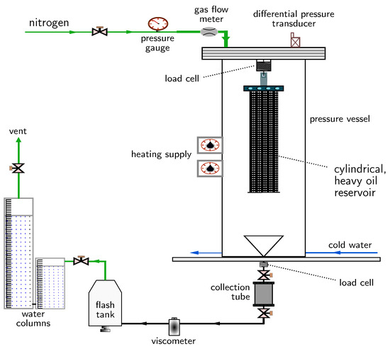
Figure 1.
Schematic of a labscale setup for heavy oil recovery using gas injection.
3.1. Process Model
Based on first principles, the process model is given by the following three state equations:
where T is the temperature inside the reservoir, w is the mass fraction of the dissolved gas in the reservoir, Z is the time-dependent reservoir height along the vertical direction, t is time, r is radial distance, and z is the vertical or axial distance. Moreover, where and K are, respectively, the relative permeability and permeability of the reservoir, g is gravity, is oil density, and is reservoir porosity with as specific heat capacity and k as thermal conductivity.
It may be noted that is the dispersion coefficient of gas in heavy oil (refer to Appendix B), is the heavy oil viscosity (see Appendix C), and is the average viscosity at , and is a function of r. Thus, at any time is the average of the viscosity values at the corners , , and of a differential element at a given r and .
It is assumed that the flow of the live oil through the porous medium along the vertical direction is governed by Darcy’s law, gas diffusion is dominant only along the radial direction, and the porous medium has constant , , , and k in the range of temperature variation [26].
Initial and Boundary Conditions
Initially, the reservoir is at room temperature with height , and no gas mass fraction, except at the surface. Thus, initial conditions are:
The boundary conditions are the specifications of T and w at the surface, and the radial symmetric conditions as follows:
In the above equations, is the interfacial gas mass fraction (i.e., gas solubility) while is the interfacial temperature. The latter is a control function depending on time, and influences .
3.2. Open Loop Optimal Control Problem
This problem involves the maximization of heavy oil production, i.e., the objective functional
using interfacial temperature versus time, , as a control function. Here, is the rate of recovery of the heavy oil from the bottom of the reservoir.
The maximization of I is equivalent to the maximization of the augmented functional
which is obtained by adjoining I to the state equations, Equations (15)–(17), with the help of the three undetermined costate variables—, , and .
3.2.1. Control Function
It may be noted that the control function is the temperature at:
- the curved surface, i.e., for any height and time;
- the bottom surface, i.e., for any radial distance and time; and
- the top surface, i.e., for any radial distance and time.
3.2.2. Necessary Conditions for Optimality
At the optimum, . This gives rise to the necessary conditions that must be satisfied by the control function, , to be optimal. The conditions are the state equations, costate equations, and the stationarity conditions as follows.
- Costate Equations These equations are:where for a property x, denotes the average x in the differential element at a given r and ; and subscripted r and z denote partial differentiation, e.g., , , etc.The costate equations are subject to the following terminal and boundary conditions:
- Stationarity Condition This stems from zeroing out the variational derivative of J with respect to , and is as follows:
3.2.3. Computational Algorithm
The following computational algorithm was executed to determine optimal, open loop control policy at a given pressure:
- Provide an initial guess for control values at each sample time instant in the interval.
- Integrate the state equations forward using the initial and boundary conditions and the control values. Save the values of state variables at all sample time instants and spatial grid points.
- Evaluate the objective functional. If the relative increase in its value is less than , quit with the control values, which are optimal.
- Integrate the costate equations backward using the terminal and boundary conditions, and the values of control and the saved state variables. Save the values of costate variables at all sample time instants and spatial grid points.
- Compute the left hand side of the stationarity condition at each sample time to obtain the gradient, and use it to improve the control values.
- Go to Step 2 and repeat computations with the improved control values.
We applied the second order finite-difference approximations along the radial and axial directions to the partial differential, state and costate equations (PDEs). This step yielded a set of ordinary differential equations (ODEs) for each PDE at the grid points. The ODEs were then integrated using the fifth order Runge–Kutta–Fehlberg method with adaptive step-size control [27]. Grid-independence analysis was done to determine adequate number of grid points to be used in computations [24]. Broyden–Fletcher–Goldfarb–Shanno (BFGS) method [28] was utilized to improve the control values. The computational algorithm was programmed in C++, and executed on a desktop computer with Intel Core-I7 processor (64 bit, 3.60 GHz and 15.9 GB usable RAM). Appendix D provides the parameter values used in the computations.
3.2.4. Open Loop Results
The above algorithm was applied for five different pressures—24.5, 43.5, 50, 58.5, and 74.5 psi. In addition, operating temperature ranged from 25.0 °C to 90.0 °C. These operating ranges for pressure and temperature were selected based on the design limitations of the experimental apparatus used to validate the process model in previous studies [26,29,30]. At each pressure, the algorithm was executed several times with different initial guesses using 30 control values equispaced over the 163.9 min time interval. It was found that the algorithm converged to the same, final values of control versus time at a given pressure.
Figure 2 shows the control values thus obtained. The corresponding values of optimal oil mass, and computation time and iterations taken by the algorithm are shown in Table 1.
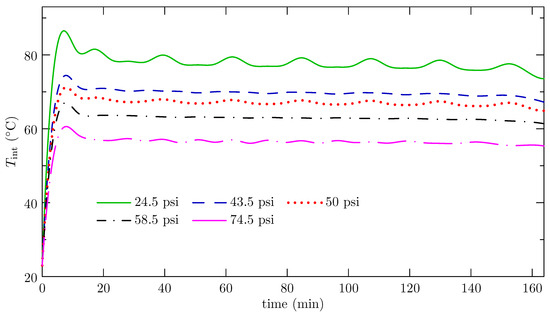
Figure 2.
Optimal, open loop control policies, i.e., optimal , at different pressures.

Table 1.
Optimal I (i.e., recovered oil mass) under open loop control at different pressures, and the corresponding computational overhead.
It is observed that as pressure increases from 24.5 psi to 74.5 psi, value of optimal I increases from 19.3 to 58.3 , whereas the average optimal decreases from 77.9 °C to 56.6 °C. This result indicates that a higher pressure causes more gas to penetrate the reservoir and increase oil recovery. In addition, a lower gas temperature is more conducive to oil recovery at a higher pressure.
It may be noted that after quickly achieving a maximum, the optimal becomes mildly wavy in nature. Such behavior leads to temporary reversals in temperature and concentration gradients, which have been found to augment oil recovery in past studies [26,29,31].
Based on these optimal open loop results, we now implement closed loop control in presence of pressure upsets in the range, 24.5–74.5 psi.
3.3. Closed Loop Optimal Control
Following the development of Section 2, the Hamiltonian associated with Equation (25) is given by
where the two states (T and w), costates ( and ) as well as their spatial derivatives span the radial and axial directions, which are discretized using equispaced grid points indexed, respectively, by subscripts i and j. The third state (Z) and the costate () span the radial direction only.
3.3.1. Control Methodology
For the online control of the process, we proceeded as follows. Right after the convergence of the open loop algorithm in Section 3.2.3 for a given pressure, the differential Riccati equation, Equation (12), was integrated based on the Hamiltonian given by Equation (34), and the gain matrix was computed from Equation (14). In this way, a repository of the optimal states and gains was obtained for five pressures, i.e., 24.5, 43.5, 50, 58.5, and 74.5 psi.
Next, the following online computational algorithm was executed for the closed loop control of the process, which was subjected to single or multiple step changes in pressure:
- Begin the process simulation at a specified pressure, and apply the open loop, optimal control values determined earlier.
- When there is or has been a pressure upset, replace the current control withwhere is the current state while and are the gain and optimal state at the new pressure. The last two items are interpolated from the pre-determined repository of optimal states and gains.
- Go to Step 2 at the next sample time.
Both open loop and closed loop algorithms are portrayed in Figure 3.
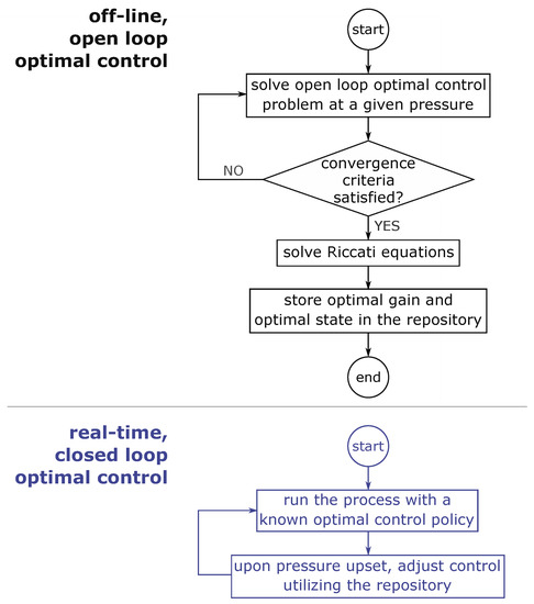
Figure 3.
Open loop and closed loop optimal control algorithms.
3.3.2. Results
In this section, we present the results obtained from the application of the developed control methodology on the heavy oil recovery process subjected to one or more pressure upsets or step changes.
Figure 4 shows the results for the closed loop control of the process after a step change of 17% in the initial pressure—from 50 psi to 58.5 psi—at 22.6 min. The open loop, optimal control policies at the five different pressures are also shown. It is observed that the control after the pressure upset approaches in about 27 min to the optimal policy corresponding to the new pressure. This adjustment leads to an improvement in the objective functional value, i.e., oil recovery. It gets raised from 42.6 g (at 50 psi without upset) to 51.0 g, which is close to 52.8 g (at 58.5 psi without upset).
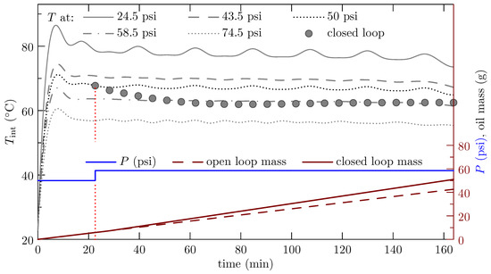
Figure 4.
Closed loop control of the oil recovery process with a pressure upset at 22.6 min.
Figure 5 shows the results for a process run similar to the previous one but with the upset delayed to 73.5 min. It is observed that the control takes about the same time to approach the optimal policy for the new pressure, and yields 48 g of oil. This value is higher than that for 50 psi but lower than that in Figure 4. This is reasonable as the process is subjected to higher pressure (which facilitates oil recovery) but for a shorter duration though, due to the delayed pressure upset.
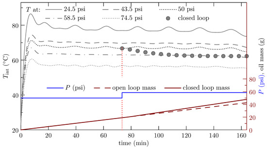
Figure 5.
Closed loop control of the oil recovery process with a delayed pressure upset at 73.5 min.
Figure 6 shows the results for the process initiated at 50 psi, and then subjected to five pressure upsets of 52.5, 56, 58.5, 62.5, and 67.5 psi at, respectively, 28.3, 39.6, 56.5, 73.5, and 84.8 min. It is observed that the control begins to decrease with the onset of pressure upsets, which are all positive. This is expected since lower control values are optimal at higher pressures. The oil recovery is 54.8 g, which lies between objective functional values of the neighborhood pressures, i.e., 52.8 g (for 58.5 psi) and 58.3 g (for 74.5 psi).
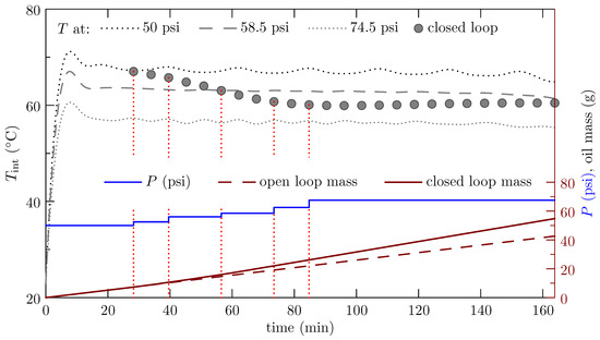
Figure 6.
Closed loop control of the oil recovery process with multiple pressure upsets.
Tracking Property
To examine the tracking property of the control methodology, we consider the process control run of Figure 5, which is subjected to 17% pressure increment at 73 min. Figure 7 plots the reservoir temperature at the grid point: (). It is observed that the temperature under feedback control progressively approaches the optimal reservoir temperature for that grid point at the new pressure.
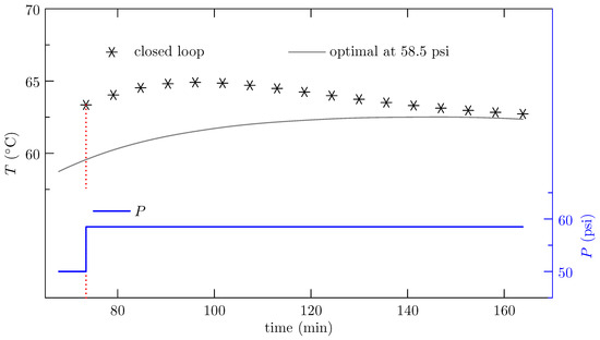
Figure 7.
Temperature inside the oil reservoir at the grid point corresponding to and .
For all grid points, Figure 8 plots the square of the error between the reservoir temperature under feedback control, and the corresponding optimal temperature at the new pressure. It is observed that the errors tend to insignificant values with time as the controlled state tracks the optimal state corresponding to the new pressure. The time derivative of the plotted error is of the order in the end. These results demonstrate that the developed control methodology has the capability to steer the process to the new optimum in case of a pressure upset.
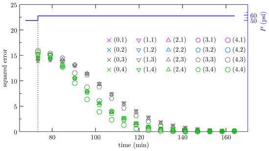
Figure 8.
Square of the error—between the feedback-controlled temperature, and the optimal temperature at the new pressure—at different grid points in the oil reservoir.
Computational Overhead
With the modest computer configuration described in Section 3.2.3, it took less than a microsecond to carry out online computations to determine and apply a feedback correction to control.
Thus, the online feedback control has negligible time delay, which is very beneficial since it helps minimize the propagation of the effects of upsets on a process. As to storage requirements, it may be noted that the repository, which was determined offline, required a total space of just 0.185 MB.
Overall, the results indicate that the proposed control methodology has a potential for real-time, feedback control of non-linear and distributed-parameter processes. This methodology has the ability to take control action with minimal time delay, and track the optimal state. Of course, the field implementation would require suitable instrumentation including soft sensors for online state measurement/estimation at different grid point locations of the system.
4. Conclusions
Based on the perturbation from an optimal state, a closed loop control strategy was developed for non-linear, distributed-parameter processes. The strategy incorporates offline computation of a repository of open-loop optimal states and gains corresponding to different values of a parameter susceptible to upsets. When an upset in the parameter occurs, control adjustments are quickly determined from the repository to attain the new optimal state.
The strategy was applied to a highly non-linear process of gas-based heavy oil recovery with three states varying with space and time in a moving boundary scenario. The objective was to maximize the oil recovery using gas temperature versus time as the control function with pressure subjected to upsets. Single and multiple pressure upsets were applied in process simulations, and relevant control adjustments were made on the basis of the pre-computed repository of optimal states and gains, which occupied a modest space of 0.185 MB. In each case, the process attained the final, optimal state corresponding to the last value of the disturbed parameter. The time taken to compute control adjustments was less than a microsecond on a desktop computer with Intel Core-I7 processor (64 bit, 3.60 GHz and 15.9 GB usable RAM). These results suggest that the developed strategy can be promising for the real-time control of non-linear, distributed-parameter processes.
Author Contributions
D.D. derived, programmed and checked all equations for closed loop control in Application; did experiments to generate relevant data; and prepared the manuscript. S.R.U. conceptualized the optimal control problem; and helped with computational aspects and manuscript preparation.
Funding
This research received no external funding.
Conflicts of Interest
The authors declare no conflict of interest.
Nomenclature
| specific heat capacity, J g−1 °C−1 | |
| D | dispersion coefficient of gas in heavy oil, cm2 min−1 |
| vector of right hand side of state equations | |
| g | gravity, cm min−2 |
| H | Hamiltonian |
| I | objective functional |
| J | augmented functional |
| k | thermal conductivity, J cm−1 min−1 °C−1 |
| K | permeability |
| relative permeability | |
| gain matrix | |
| mass flow rate of oil, g min−1 | |
| r | radial distance, cm |
| Riccati matrix | |
| t | time, min |
| final time, min | |
| T | temperature, |
| T at gas–heavy oil interface, | |
| control vector | |
| v | Darcy velocity, cm min−1 |
| w | gas mass fraction in heavy oil reservoir |
| w at gas–heavy oil interface | |
| average value of x | |
| optimal vector | |
| state vector | |
| z | axial distance, |
| Z | height of the cylindrical, heavy oil reservoir, cm |
| Z at , cm | |
| Greek Letters | |
| thermal diffusivity, cm2 min−1 | |
| variation of x | |
| variation of vector | |
| distance between consecutive radial grid points, | |
| distance between consecutive axial grid points, | |
| costate vector | |
| viscosity of heavy oil, g cm−1 min−1 | |
| density of heavy oil, g cm−3 | |
| porosity of heavy oil reservoir | |
Appendix A. Gas Solubility Data
From the data of dissolved gas (nitrogen) in heavy oil, the gas solubility () was determined as a function of temperature and pressure. For this purpose, the selected operating pressures were 24.5, 43.5, 50, 58.5 and 74.5 psi. For each of these pressures, experiments were performed at 25, 50, 75 and 90 . Figure A1 shows the gas solubility thus obtained. It is observed that it rises with both temperature and pressure.

Figure A1.
Solubility of gas (nitrogen) versus temperature at different pressures.
Figure A1.
Solubility of gas (nitrogen) versus temperature at different pressures.

Appendix B. Dispersion Coefficient of Gas
The dispersion coefficient of gas (nitrogen) was determined as a function of its mass fraction in heavy oil utilizing a method developed elsewhere [30,32]. Shown in Figure A2, the dispersion coefficient increases with the mass fraction to a maximum and drops subsequently.


Figure A2.
Dispersion coefficient of nitrogen versus its mass fraction in heavy oil at different temperatures and pressures.
Figure A2.
Dispersion coefficient of nitrogen versus its mass fraction in heavy oil at different temperatures and pressures.


Appendix C. Heavy Oil Viscosity
The following correlation was used for the viscosity of heavy oil as a function of temperature (), pressure (psi), and the gas (nitrogen) mass fraction:
The parameter values in the above equation are:
| Parameter | |||||||||
| value | 0.44 | −61.19 | 2533.90 | −0.05 | −16.17 | 2950.30 | 0.15 | −7.96 | 160.00 |
Appendix D. Parameters used in Computations
| Parameter | Value |
| specific heat capacity of heavy oil () | 2.13 J g−1 °C−1 |
| diameter of the physical model (D) | 5.5 |
| gravity (g) | 35,31,600 cm min−2 |
| thermal conductivity of heavy oil (k) | 0.6 J cm−1 min−1 °C−1 |
| permeability of reservoir (K) | 4 Darcy |
| relative permeability of revervoir () | 1 |
| number of radial grid points () | 6 |
| number of axial grid points () | 6 |
| room temperatures () | 23 |
| initial height of the physical model () | 35 |
| density of heavy oil () | 0.821 g cm−3 |
References
- Diehl, M.; Bock, H.G.; Schlöder, J.P.; Findeisen, R.; Nagy, Z.; Allgöwer, F. Real-time optimization and nonlinear model predictive control of processes governed by differential-algebraic equations. J. Process Control 2002, 12, 577–585. [Google Scholar] [CrossRef]
- De Souza, G.; Odloak, D.; Zanin, A.C. Real time optimization (RTO) with model predictive control (MPC). Comput. Chem. Eng. 2010, 34, 1999–2006. [Google Scholar] [CrossRef]
- Huang, R.; Biegler, L.T.; Patwardhan, S.C. Fast offset-free nonlinear model predictive control based on moving horizon estimation. Ind. Eng. Chem. Res. 2010, 49, 7882–7890. [Google Scholar] [CrossRef]
- Adetola, V.; Guay, M. Integration of real-time optimization and model predictive control. J. Process Control 2010, 20, 125–133. [Google Scholar] [CrossRef]
- Bonvin, D.; Srinivasan, B. On the role of the necessary conditions of optimality in structuring dynamic real-time optimization schemes. Comput. Chem. Eng. 2013, 51, 172–180. [Google Scholar] [CrossRef]
- Kamaraju, V.; Srinivasan, B.; Chiu, M. NCO-tracking based control of semi-batch antisolvent crystallization processes in the presence of uncertainties. In Proceedings of the 2013 European Control Conference (ECC 2013), Zurich, Switzerland, 17–19 July 2013; pp. 3390–3395. [Google Scholar]
- Sun, M.; Chachuat, B.; Pistikopoulos, E.N. Design of multi-parametric NCO tracking controllers for linear dynamic systems. Comput. Chem. Eng. 2016, 92, 64–77. [Google Scholar] [CrossRef]
- Findeisen, R.; Allgöwer, F. Computational Delay in Nonlinear Model Predictive Control. IFAC Proc. Vol. 2004, 37, 427–432. [Google Scholar] [CrossRef]
- Wolf, I.J.; Marquardt, W. Fast NMPC schemes for regulatory and economic NMPC—A review. J. Process Control 2016, 44, 162–183. [Google Scholar] [CrossRef]
- Pesch, H. Real-time computation of feedback controls for constrained optimal control problems. Part 2: A correction method based on multiple shooting. Opt. Control Appl. Methods 1989, 10, 147–171. [Google Scholar] [CrossRef]
- Pesch, H. Real-time computation of feedback controls for constrained optimal control problems. Part 1: Neighbouring extremals. Opt. Control Appl. Methods 1989, 10, 129–145. [Google Scholar] [CrossRef]
- Domínguez, L.; Pistikopoulos, E. Recent Advances in Explicit Multiparametric Nonlinear Model Predictive Control. Indu. Eng. Chem. Res. 2011, 50, 609–619. [Google Scholar] [CrossRef]
- Aydin, E.; Bonvin, D.; Sundmacher, K. Dynamic optimization of constrained semi-batch processes using Pontryagin’s minimum principle—An effective quasi-Newton approach. Comput. Chem. Eng. 2017, 99, 135–144. [Google Scholar] [CrossRef]
- Stengel, R. Optimal Control and Estimation; Dover Publications Inc.: New York, NY, USA, 1994; Chapter 3. [Google Scholar]
- François, G.; Srinivasan, B.; Bonvin, D. Use of measurements for enforcing the necessary conditions of optimality in the presence of constraints and uncertainty. J. Process Control 2005, 15, 701–712. [Google Scholar] [CrossRef]
- Upreti, S. Optimal Control for Chemical Engineers; CRC Press: Boca Raton, FL, USA, 2013; Chapter 7. [Google Scholar]
- Lions, J. The optimal control of distributed systems. Russ. Math. Surv. 1973, 28, 13–46. [Google Scholar] [CrossRef]
- Omatu, S.; Seinfeld, J.H. Distributed Parameter Systems, Theory and Applications; Clarendon Press: Oxford, UK, 1989. [Google Scholar]
- Tröltzsch, F. Optimal Control of Partial Differential Equations: Theory, Methods, and Applications; American Mathematical Society: Providence, RI, USA, 2010; Volume 112. [Google Scholar]
- Rad, J.; Kazem, S.; Parand, K. Optimal control of a parabolic distributed parameter system via radial basis functions. Commun. Nonlinear Sci. Numer. Simul. 2014, 19, 2559–2567. [Google Scholar] [CrossRef]
- Kotsur, M. Optimal control of distributed parameter systems with application to transient thermoelectric cooling. Adv. Electr. Comput. Eng. 2015, 15, 117–123. [Google Scholar] [CrossRef]
- Alessandri, A.; Gaggero, M.; Zoppoli, R. Feedback optimal control of distributed parameter systems by using finite-dimensional approximation schemes. IEEE Trans. Neural Netw. Learn. Syst. 2012, 23, 984–996. [Google Scholar] [CrossRef]
- Nosratipour, H.; Sarani, F.; Fard, O.S.; Borzabadi, A.H. An adaptive nonmonotone truncated Newton method for optimal control of a class of parabolic distributed parameter systems. Eng. Comput. 2019. [Google Scholar] [CrossRef]
- Dutta, D. Real Time Optimal Control of Distributed-Parameter Systems. Master’s Thesis, Ryerson University, Toronto, ON, Canada, 2019. [Google Scholar]
- Aadnoy, B.S. Modern Well Design; CRC Press: Boca Raton, FL, USA, 2010. [Google Scholar]
- Booran, S. Optimal Control of Atmospheric Air Injection for Enhanced Oil Recovery. Ph.D. Thesis, Ryerson University, Toronto, ON, Canada, 2017. [Google Scholar]
- Press, W.H.; Teukolsky, S.A.; Vetterling, W.T.; Flannery, B.P. Numerical Recipes in C++: The Art of Scientific Computing; Cambridge University Press: Cambridge, UK, 2002. [Google Scholar]
- Dai, Y.H. A perfect example for the BFGS method. Math. Programm. 2013, 138, 501–530. [Google Scholar] [CrossRef]
- Muhamad, H.; Upreti, S.R.; Lohi, A.; Doan, H. Performance enhancement of VAPEX by varying the propane injection pressure with time. Energy Fuels 2012, 26, 3514–3520. [Google Scholar] [CrossRef]
- Abukhalifeh, H.; Lohi, A.; Upreti, S. A novel technique to determine concentration-dependent solvent dispersion in VAPEX. Energies 2009, 2, 851–872. [Google Scholar] [CrossRef]
- Muhamad, H.; Upreti, S.R.; Lohi, A.; Doan, H. Optimal control study to enhance oil production in labscale Vapex by varying solvent injection pressure with time. Opt. Control Appl. Methods 2016, 37, 424–440. [Google Scholar] [CrossRef]
- Abukhalifeh, H.; Upreti, S.R.; Lohi, A. Effect of drainage height on concentration-dependent propane dispersion in vapex. Can. J. Chem. Eng. 2012, 90, 336–341. [Google Scholar] [CrossRef]


© 2019 by the authors. Licensee MDPI, Basel, Switzerland. This article is an open access article distributed under the terms and conditions of the Creative Commons Attribution (CC BY) license (http://creativecommons.org/licenses/by/4.0/).