Article

A Numerical Research on Vortex Street Flow Oscillation in the Double Flapper Nozzle Servo Valve

1
School of Mechanical Engineering, Tongji University, Shanghai 200092, China
2
Shanghai Institute of Aerospace Control Technology, Shanghai 201109, China
3
Shanghai Servo System Engineering Technology Research Center, Shanghai 201109, China
*
Author to whom correspondence should be addressed.
Processes 2019, 7(10), 721; https://doi.org/10.3390/pr7100721
Submission received: 27 August 2019 / Revised: 7 October 2019 / Accepted: 8 October 2019 / Published: 11 October 2019
(This article belongs to the Special Issue Smart Flow Control Processes in Micro Scale)

Abstract

:
The oscillating flow field of the double nozzle flapper servo valve pre-stage is numerically analyzed through Large Eddy Simulation (LES) turbulent modeling with the previous grid independence verification. The vortex street flow phenomenon can be observed when the flow passes through the nozzle flapper channel, the vortex alternating in each side produces the periodical flow oscillation. The structural and flow parameter effects on the oscillating flow are emphasized, and it could be determined that the pressure on the flapper is nearly proportional to the flow velocity and inversely proportional to the actual distance between the flapper and the nozzle. On the other hand, the main frequency of oscillation decreases with the velocity and increases with the distance between the nozzle flapper. The main stage movement is further considered with a User Defined Function (UDF), and it could be determined that the influences of the structural and flow parameters on the flow oscillation are rarely changed, but the main frequencies drop, generally.

1. Introduction

As the core component of hydraulic control systems, the electro-hydraulic servo valve has certain advantages of high performance and high reliability. Its first appearance was to the application in fighter planes during World War II, but the single-stage open-loop structure made it difficult to meet the control requirements at that time [1]. It was not until Massachusetts institute of technology (MIT) replaced the solenoid with a high-frequency permanent magnet torque motor that the servo valve ushered in its golden period of development. In 1953, the single nozzle flapper valve was firstly invented by Moog [2]. After four years, the single nozzle structure was further improved to have double nozzles by Howard [3]. In 1962, Atchley [4] invented the jet tube servo valve. Thanks to the development of electronic technology, Vanderlaan et al. [5] made the servo motors directly drive the spool movement in 1987. In 1993, Laux [6] improved and invented the rotary direct drive servo valve. However, the direct drive servo valves are still limited by insufficient motor power, leading to the frequency response not being quick enough. With the advantages of a high power density ratio and a high frequency response, jet servo valves are still popularly applied in crucial industrial applications, including aerospace, ship engineering, high-end robots, etc. At present, research on jet servo valves are still in progress.
There are many related aspects of servo valve research. For example, on the control algorithm, Samakwong et al. [7] found that a genetic algorithm (GA) could better optimize the parameters of the PID controller and control the performance of the servo valve than the Ziegler–Nichols adjustment method. With respect to mathematical modeling, Brito et al. [8] established a Hammerstein model for aerospace servo valves, the results showing that the identified model can represent the general non-linear behavior of servo valves. With respect to hydraulic power, Zohreh et al. [9] simulated the valve core pressure under unsteady conditions. It was found that in the two-stage flapper nozzle electro-hydraulic valve the external acceleration would change the fluid pressure leaving the nozzle and produce the same effect as the external force. Ye et al. [10] established the dynamic model of the plunger pump, simulated it by Computational Fluid Dynamics (CFD), and verified it experimentally. The results show that the vibration speed of the plunger pump on the XF axis is higher than that on the YF axis. The excitation moment MCY and MPY on the YF axis contribute greatly to the vibration of the plunger pump. On the flow field characteristic, many scholars adopted CFD approaches to obtain the complex valve flow detail. Brito et al. [8] also carried out experimental and numerical studies to determine the mechanism of cavitation in the fluid region between the flapper and nozzle by using 3D models and CFD grids. Li et al. [11] observed the cavitation phenomena in the flow field from Reynolds numbers 630–2500 with the comparison of CFD simulation. They found that the computational results were in good agreement with the experimental observations and came to the conclusion that the position of the cavitation source is shown at the tip of the nozzle inner wall, the tip of the nozzle outer wall, and the front of the flapper. Chen et al. [12] revealed the effect of oil viscosity on the transient distribution of cavitation and small-size vortices, indicating the noise accompanied by the flow resonance in the nozzle. When the pressure fluctuation near the flowmeter is large enough in the two-stage servo valve, flow acoustic resonance and screaming may occur. Qian et al. [13] researched the forward and reverse flow of Al2O3-water nanofluids in micro T45-R Tesla valves at different flow rates, temperatures, and nanoparticle volume fractions by CFD on the basis of the verified numerical model, finding that the main flow percentage was proportional to the above three factors and the flow rate has the greatest influence on the polarity of the valve. Chao et al. [14] found that the inward inclined design of cylinder ports could effectively decrease the gaseous cavitation and increase the effective output flow of cylinder by using centrifugal effects of rotating fluid, which provided a new way to optimize the performance of (Electro-Hydrostatic Actuator) EHA. Qian et al. [15] used CFD to simulate the valve core diameter, single hole/porous diameter, hole diameter, and its arrangement at the bottom of the valve core steadily and instantaneously, and found that the pressure difference between the two sides increases with the increase of the diameter of the valve core and the decrease of the aperture. Meanwhile, the opening time of the main valve also increases with the increase of the diameter of the valve core. Zhang et al. [16] proposed a damping sleeve with a throttle hole. Through experiments and numerical calculation, it was found that the designed damper sleeve had a significant effect on the pressure distribution and jet direction on the surface of the cone, which can significantly reduce the flow force and the opening time of the valve.
Recently, with the improvement of working requirements, the jet flow velocity comes to a higher level with a larger Mach number. The flow compressible effect is more and more obvious. The authors acknowledge there are rarely any studies that have paid enough attention to the high-speed compressible flow oscillations in the jet servo valves. For the present paper content organization, the CFD approach is employed with a (Large Eddy Simulation) LES turbulent model to obtain the vortex flow oscillation conditions. After determining the independence of the grid, the flow field of the fluid in the servo valve with double nozzles and flappers is analyzed under the condition of changing the inlet oil flow rate and the deflection displacement of the flappers, while the force acting on the servo valve flappers under the coupling of the main valve is also discussed.

2. Flow Structure and Grid Independence Analysis

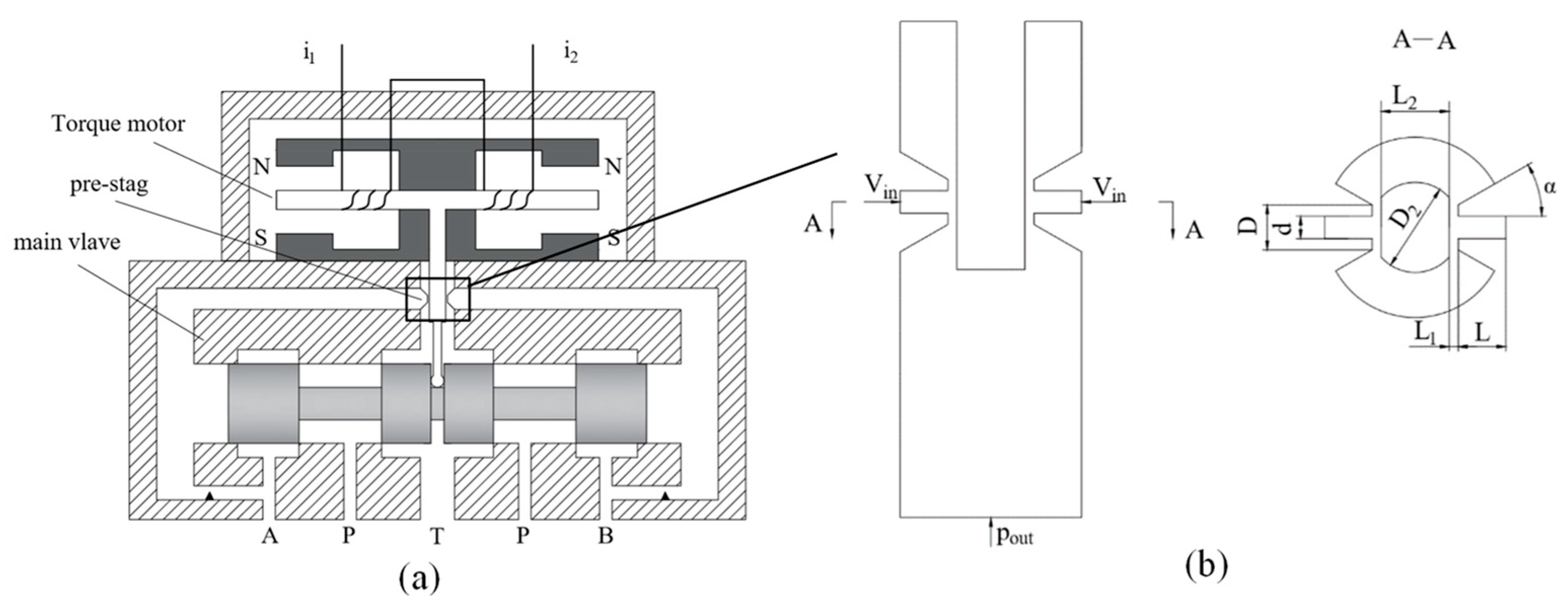
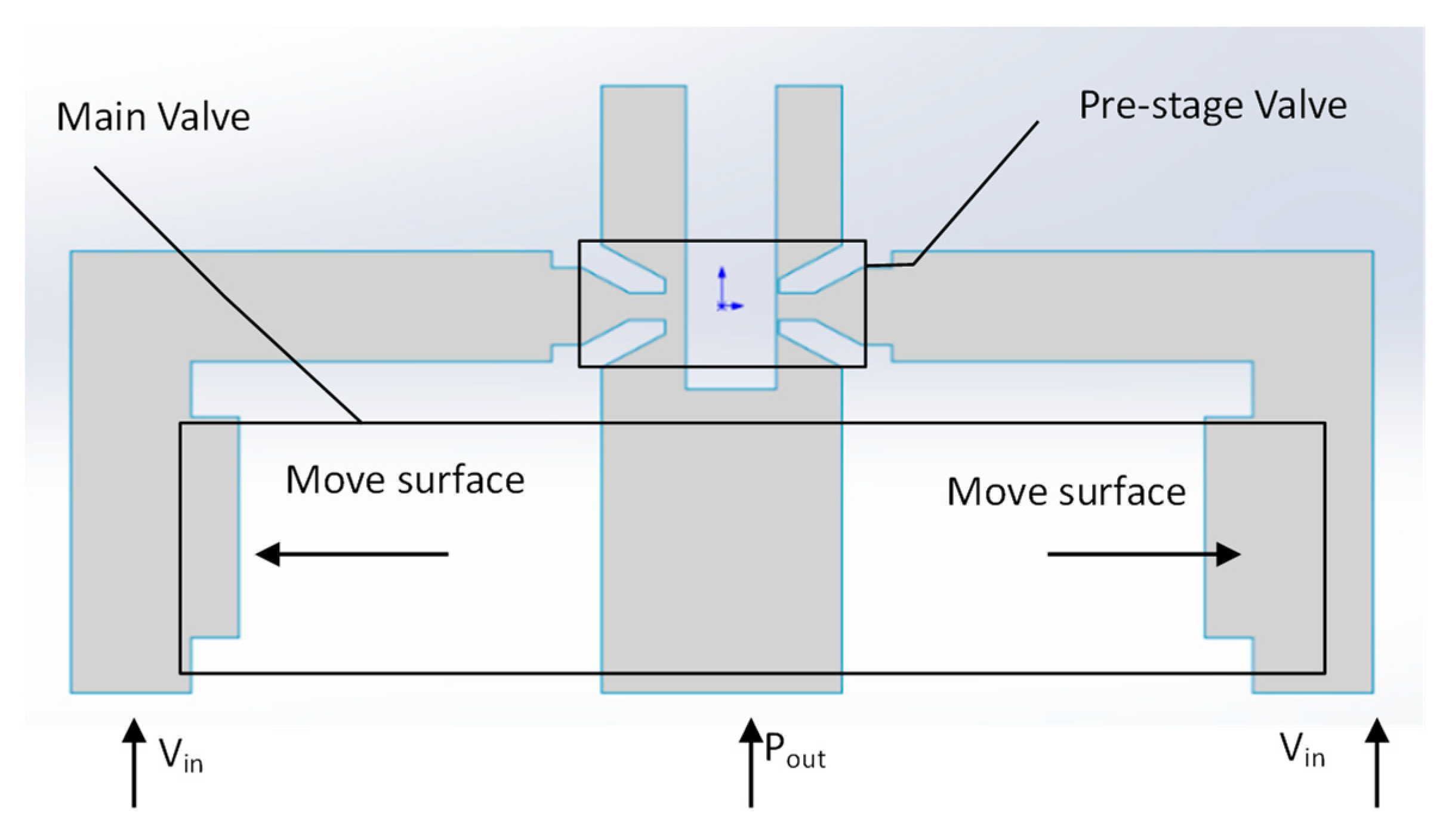
2.1. Operation Principle and Structural Parameters

The two-stage double nozzle flapper force feedback electro-hydraulic servo valve is taken as the research object. As shown in Figure 1a, when the servo valve is in the initial position, the coil is not electrified, the flapper is located in the middle of the nozzle without deflecting, the flow force acting on the flapper is offset each other, the pressure loss caused by the variable throttle hole is the same, the pressure at both ends of the main valve core is the same, and the main valve core is not moving. When the corresponding electric signal is input, the coil generates a magnetic field, which makes the torque motor produce a magnetic moment, and drives the flapper to produce the corresponding deflection angle, thus promoting the movement of the main valve core. As shown in Figure 1b, the simplified structure of the jet location, when the current flowing through the left and right coils is different, for example of i1 > i2, the electromagnetic moment produced by the left coil is larger than that of the right coil, which makes the coil rotate clockwise, and makes the flapper shift to the left, thus making the distance between the flapper of the jet flapper valve and the two nozzles different, the left side smaller and the right side large. The flow resistance of the hole changes, making the pressure loss on the left side small, the pressure large, the pressure loss on the right side large and the pressure small, so that the oil hydraulic pressure at the two ends of the main valve core is different, driving the main valve core to move to the right, generating load flow and driving the load operation. At the same time, the armature rotates, driving the feedback rod fixed on the armature to shift to the left. Deformation results in counter-clockwise feedback moment. The motion of the valve core makes the feedback rod more deformed and the feedback moment correspondingly larger. When the feedback moments generated by the two are superimposed on the flapper and balanced with the electromagnetic moments generated by the torque motor, the spool is in a predetermined position, and the flapper is in a balanced state. At this time, the required load flow and pressure are generated, and the servo valve is in a predetermined working state. When the load changes or external disturbance causes the spool to deviate from the balanced position, the feedback moment changes, which makes the flapper deviate from the balanced position, and the flow resistance of the variable throttle hole changes accordingly. The pressure difference between the two sides of the spool is generated again, so that the flapper moves in the direction of reducing the deviation until the spool reaches the balanced state [17].
The structural parameters of the nozzle flapper chamber and the set working oil parameters are both as shown in Table 1. According to the working conditions, the maximum working pressure of the servo valve is less than 31 MPa, and the rated flow rate is 0.48–6.9 L/min. The inlet pressure is selected according to the inlet speed. The outlet pressure is set atmospheric pressure.
The pre-stage valve in this study is perpendicular to the nozzle and is mainly affected by the force in the x-axis, i.e., the horizontal direction. While the force in the y-axis, i.e., the direction perpendicular to the paper surface, counteracts each other, and has little influence on the servo valve, it can be simulated by two-dimensional flow chart, which saves on computational resources. Moreover, it is convenient to observe the flow field changes in the channel, and it has no effect on the final simulation results. The following grid and simulation are based on the 2D model shown in Figure 1b.

2.2. Boundary Conditions and Simulation Settings

As shown in Figure 1b, there are three boundary conditions in the two-dimensional model of the flow channel, inlet, outlet, and wall. Among them, the inlet boundary is where the oil enters, Since the intensity of the change of oil flow field at the nozzle is most directly affected by the flow velocity, the inlet oil flow velocity is set as the inlet boundary condition. The outlet oil tank is set as the pressure outlet. The other surface is set as the wall. As shown in Figure 1b, Vin represents the velocity inlet, pout represents the pressure outlet, and the unspecified surfaces are all wall surfaces.
Fluent 19.0 (ANSYS 19.0, ANSYS, Inc., Canonsburg, PA, USA, 2018) is used for present numerical solution. Since there are vertical pipes in the channel model, the gravity factor should be taken into account and the gravity acceleration is 9.81 m/s2. As mentioned above, flow oscillation is a wave–vorticity coupled flow phenomenon. Therefore, when setting the fluid as a turbulent flow, compressibility must be considered, fluid state as a transient state, and the LES model is suitable for solving model. The pressure–velocity coupling term is selected as the Semi-Implicit Method for Pressure-Linked Equations Consistent (SIMPLEC) algorithm, which is improved by the SIMPLE algorithm. The correction term in the velocity equation is not neglected in each iteration. Therefore, the pressure correction value obtained is generally appropriate, and an under-relaxation coefficient less than 1 can be selected according to the situation to accelerate the convergence of the solution in the iteration process [18]. When factors such as cavitation are not considered, the oil is a single-phase flow. Since the LES model belongs to direct numerical simulation to some extent, the discrete scheme of momentum and size terms are chosen as the second-order upwind scheme with second-order accuracy. Since most of the flow field grids are quadrilateral grids and mainly focus on wave–eddy coupling, it is necessary to observe the eddy effect in turbulence, so in order to avoid errors in the difference value and the eddy effect in turbulence, the discrete scheme is adopted as the second-order upwind scheme with second-order accuracy. The pressure gradient hypothesis on the boundary is advantageous to the flexible calculation, and the pressure term is chosen as PRESTO. In order to ensure continuity, the convergence condition is defined as the third-order residuals of each parameter, and the transient equation is a second-order implicit equation. The time step is 0.0001 s, as shown in Table 2.

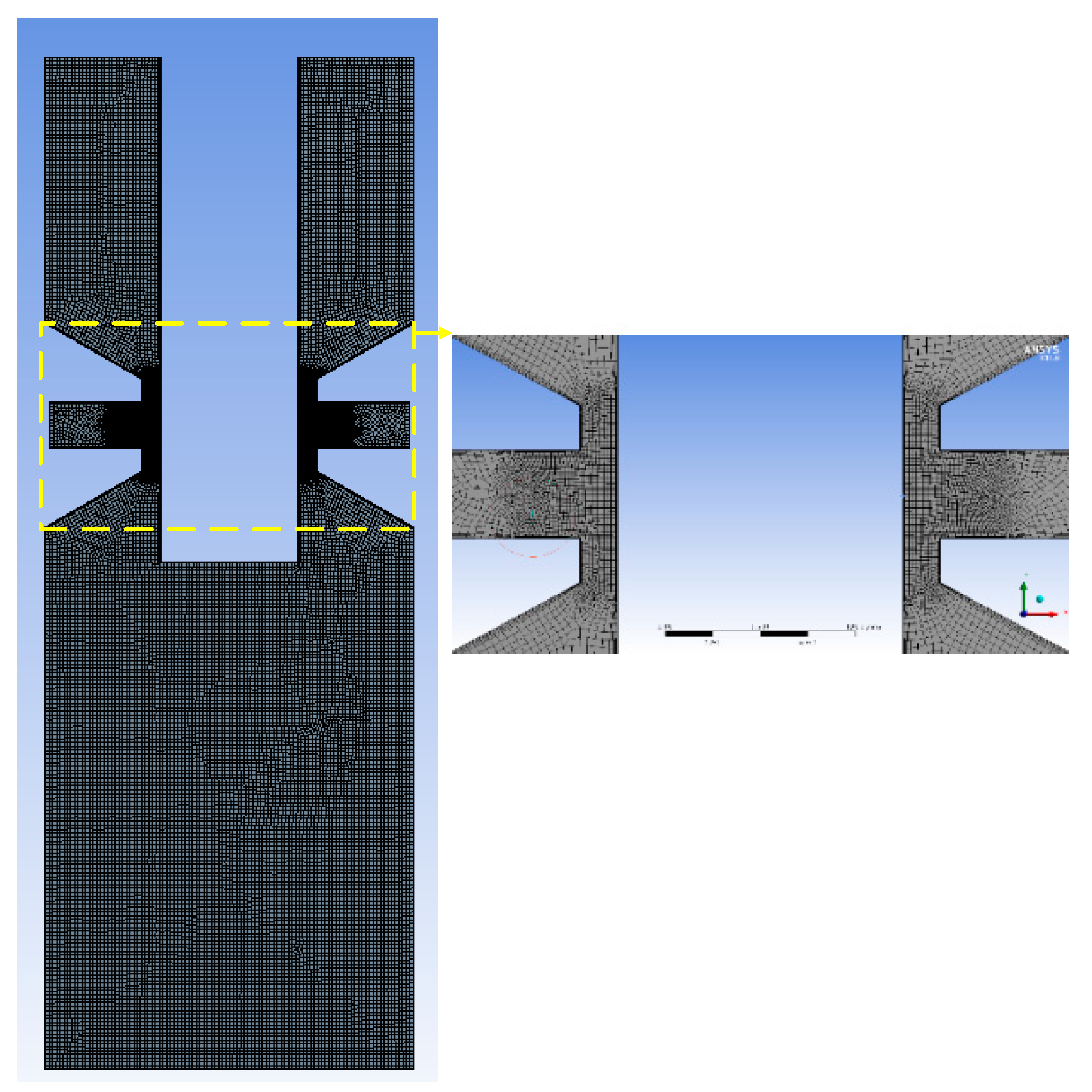
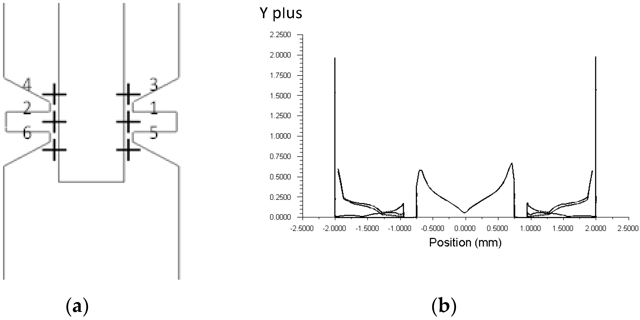
2.3. Grid Generation and Independence Analysis

The runner belongs to the regular geometric model, so the grid module of ANSYS software, mesh (ANSYS 19.0, ANSYS, Inc., Canonsburg, PA, USA, 2018) is selected to divide the runner with the Quadrilateral Dominant method. Since there are a few trapezoidal areas in the runner, the type of grid division is Quad/Tri. At the same time, the nozzle part of the key research area has a larger grid density in order to capture as many transient details as possible. The partitioned grid is shown in Figure 2, and the grid parameters are shown in Table 3.
For a servo valve, flow and pressure are the ultimate indicators, so pressure and flow can be used to determine whether the grid size is appropriate. The outlet flow and average pressure on flapper at different grid sizes are shown in Figure 3.
It can be seen that when the grid size is 0.010/0.012 and 0.015, the average pressure of the flapper is not much different, only within 0.005 MPa, while the mass flow of the outlet is almost the same, the difference being only 0.000048 kg/s. Therefore, when the grid size is in the range of 0.010–0.015, the grid quality has no effect on the simulation results. The median value of range of 0.012 is taken as the grid size when grid is independent.
After finding the optimal grid size, the channel model with different flappers are meshed. Since the distance between the flapper and the two nozzles is 0.2 mm when the flapper is located at the zero position, the number and quality parameters of the grid at different positions are obtained as shown in Table 4. The displacement of the flapper is in the right direction, i.e., the X direction shown in Figure 1 is in the positive direction.

3. Results and Discussion

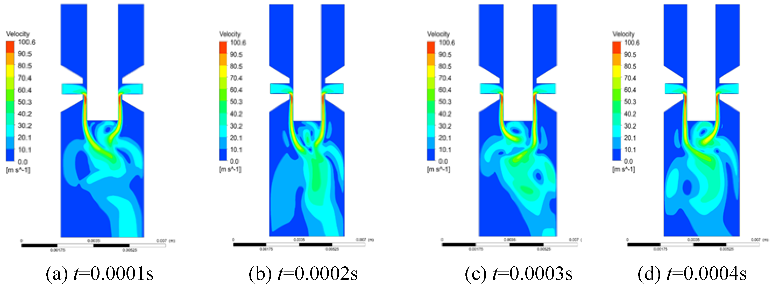
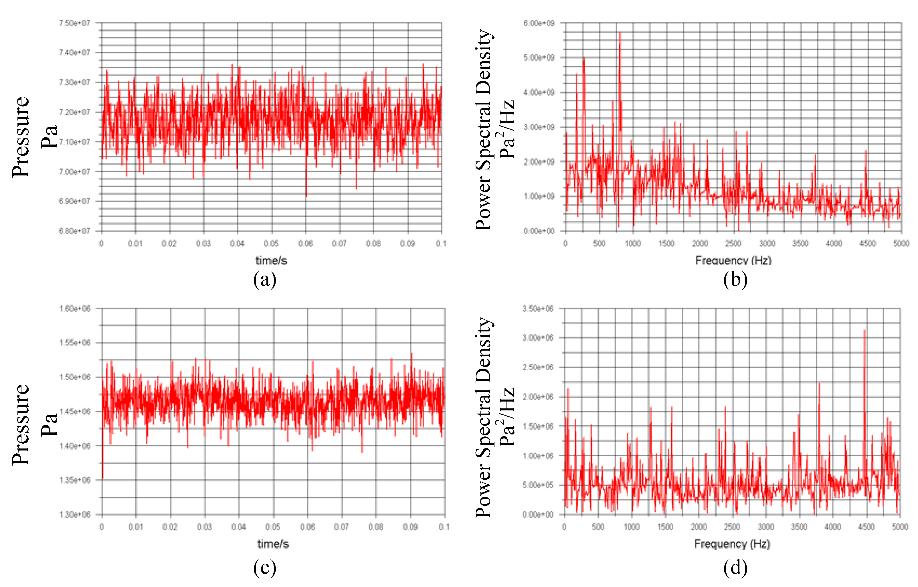
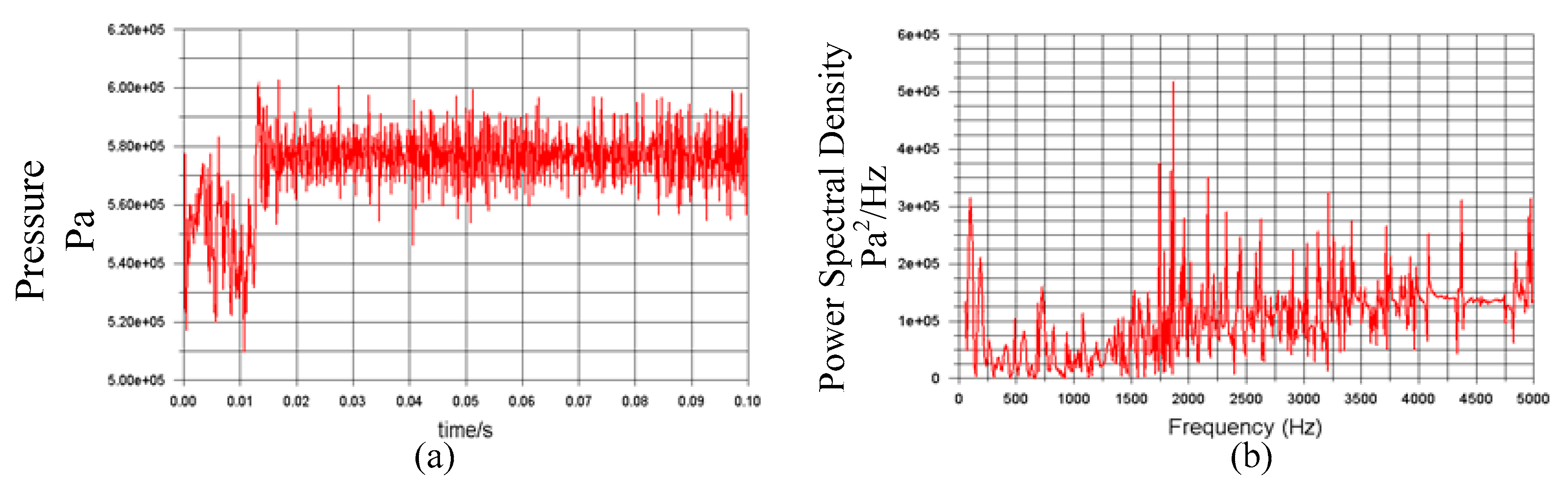
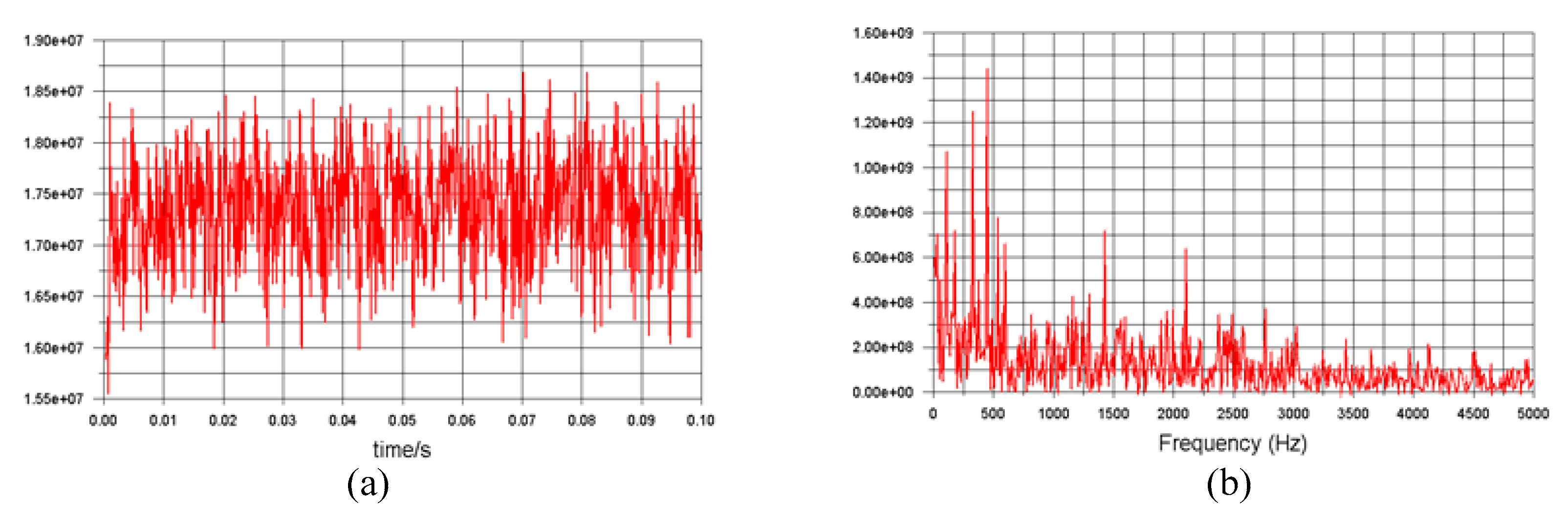
3.1. Flow Field Characteristics with Constant Velocity and Flapper Displacement

The nozzle area is selected as the observation object, and the observation points on the flow channel model are shown in Figure 4a, while Figure 4b shows that the wall Y plus number along the wall position. The results show that nearly all the wall Y plus number is less than 1 as suggested by Fluent user's guide, except for the leftmost and rightmost boundaries; however, the Y plus numbers are still less than 2. Analogously, the simulation obtained Y plus numbers in 5 m/s, 25 m/s, and 50 m/s conditions are also less than 1, mostly, including the wall areas near points 1–6, in which the research is much concerned.
The flow field model with an inlet velocity of 25 m/s and the flapper at the zero position is used for overall analysis. Since the flapper is in the zero position, the distance between the nozzles on both sides and the flapper is equal, making the flow resistance the same. According to the theoretical calculation, the pressure loss of the nozzles on both sides is the same, and the flow velocity through the nozzles should be equal. In addition, because the flow state of the oil injection to the two sides of the flapper is exactly the same, without considering the wear of the nozzles, the pressure fluctuation curves generated by the flappers on both sides should also be the same. By observing Figure 5, it is found that the oil velocity on both sides of the nozzle is the same, which is in accordance with the theory. However, in the wake region, the oil continuously makes periodic whirlpool motions, which makes the flapper subject to periodic pressure oscillations through the disturbance of the oil cycle, and in order to observe the pressure oscillation on the left and right sides of the flapper, point 1 and point 2 of Figure 4 are selected as the comparison, and the pressure situation at the two points is measured as shown in Figure 6a–d. Pressure oscillation phenomena have been observed at both points. It can be seen that there exists a fluid self-excitation oscillation between the nozzle and flapper. Moreover, the pressure oscillation curves at both points are approximately the same, the average pressure is about 0.57 MPa, and the oscillation amplitude is 0.12 MPa. Observing the power spectrum, it is found that the pressure fluctuation is mainly high frequency, and the peak frequency appears at 3000 Hz.
It is known from the foregoing that when the flapper of the jet flapper valve is located at the zero position, the average pressure, velocity and pressure fluctuation of the flapper on both sides of the flapper are almost the same, so in order to observe the pressure situation at different positions of the flapper, according to Figure 4, only points 1, 3, and 5 on the right side are selected as the observation objects. The pressure fluctuation curves are shown in Figure 6a,b,e–h respectively. From the graph analysis, it can be seen that the pressure pulsation at point 1 and point 3 oscillates around 0.57 MPa and has positive pressure, while point 5 oscillates near −0.045 MPa and the pressure is negative. This is because point 1 is located in the central region of the oil injection, so its pressure corresponds to the highest, while point 5 is located in the wake region, so the pressure is low; besides point 1, point 3, and point 5, the main frequency is low. The performance is not obvious because point 1 is the main area to be impacted by the jet, so the pressure oscillation here is also the most significant. At the same time, the pressure fluctuations in the three locations are mainly high frequency, generally over 3000 Hz, and the maximum power size appears at 3000 Hz, which indicates that the main frequency of pressure oscillation is 3000 Hz. In addition, the pressure amplitudes of the three locations are very stable in the time domain, and there is no sudden change point, which indicates that pressure oscillation exists. It is not caused by accidental factors, but by the high-speed impact of oil on the flapper.
The simulation time step is 0.0001 s, and each step is saved automatically. As a result, a flow cycle is obtained as shown in Figure 5. It can be found that the fluid disturbance is very intense when it enters the nozzle flapper area. In Figure 5a, after the fluid is injected into the nozzle flapper, it intersects at the bottom of the flapper, and the phenomenon of reflux is intensified in Figure 5b. Then a small eddy current is initially formed in Figure 5c, which is generated in Figure 5d and completes a cycle in 0.0003 s. Figure 6b shows that the main frequency is about 2850 Hz and the calculated period is about 0.00035 s, which are in good agreement with each other, indicating that the intercepted period is correct. This is because the oil continuously forms eddy currents on the flapper, producing repetitive pulses on the flapper, and thus forming a pressure oscillation on the flapper.

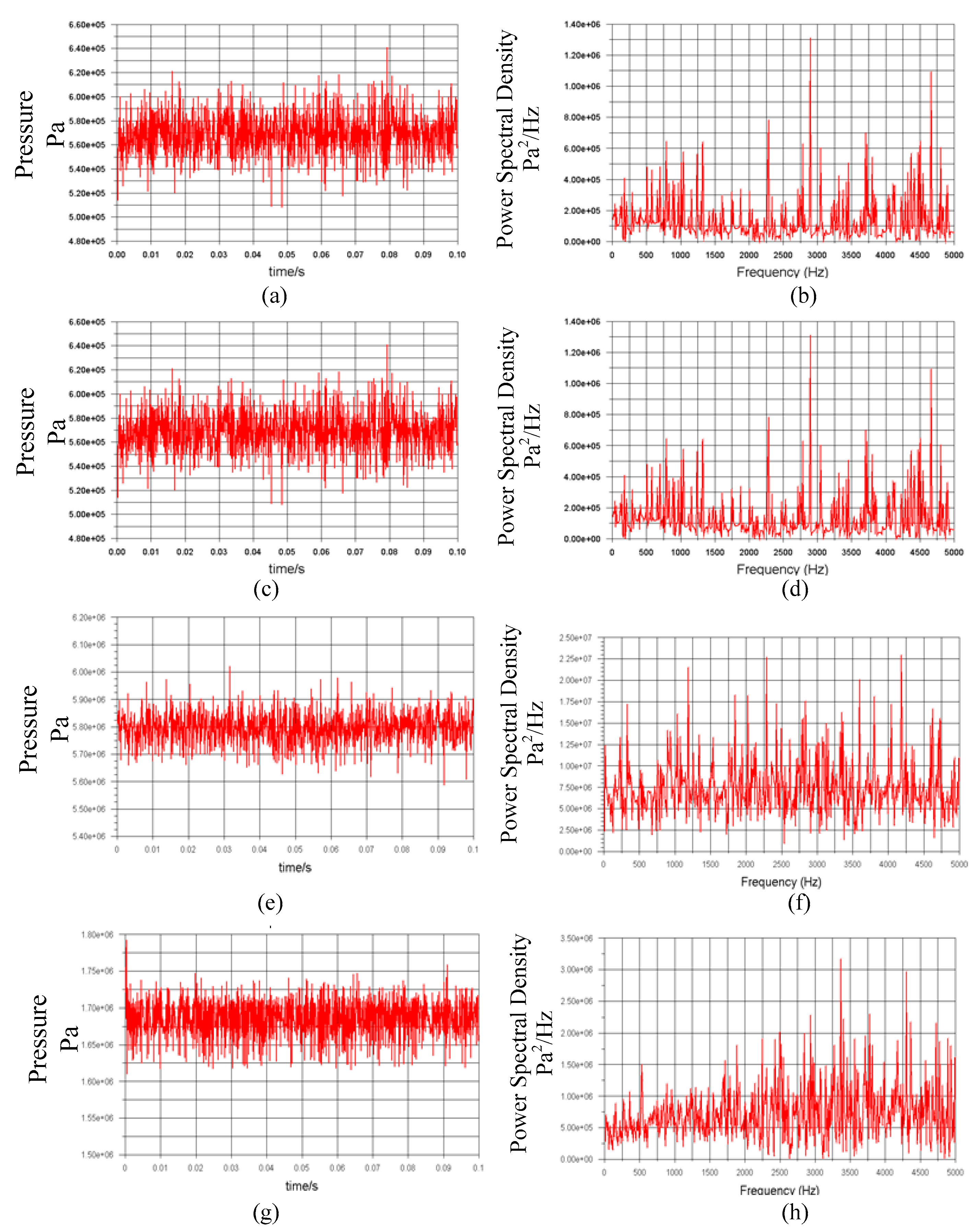
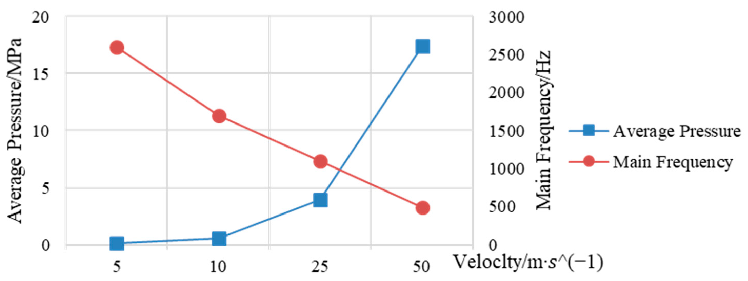
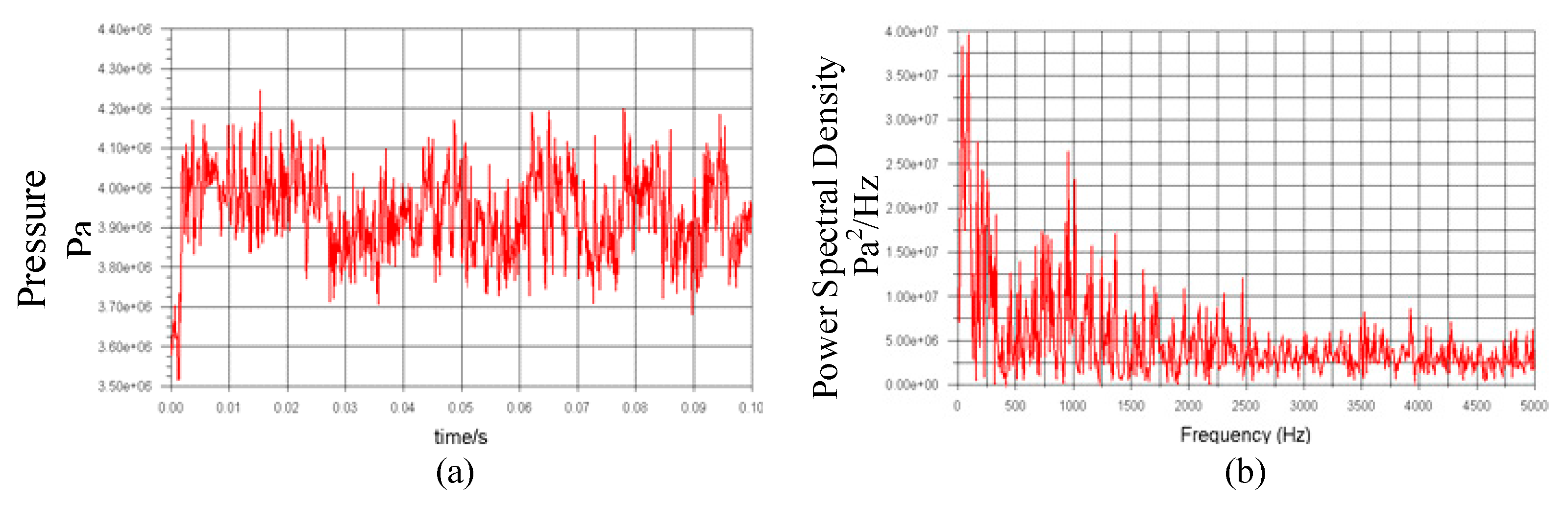
3.2. Variation of Main Frequency and Amplitude of Oscillation at Different Velocities

It can be seen from the above section that the pressure oscillation at point 1 and point 2 of the nozzles are the most obvious. Since the flapper is in the zero position and the pressure on both sides of the flapper is the same when the velocity of investigation is affected, point 1 is chosen as the research object. The results are shown in Figure 7, Figure 8, Figure 9 and Figure 10, where the figures of 20 times of l g “power spectrum density” are displayed, which show the “−5/3” slope of the frequency, much accorded with the k41 theory spectra distribution characteristic, which insures the simualtion results are turbulent, not numerical errors. After comparison, it can be found that the pressure fluctuation increases with the increase of velocity, and there is a positive correlation between them. However, with the increase in velocity, the relative oscillation amplitude of the pressure does not follow the positive correlation, but decreases with the increase of velocity. Thus, the higher the velocity of the nozzle, the pressure oscillation phase oscillation will occur. The lower the amplitude, it can be inferred that when the velocity is high enough, the pressure oscillation of the flapper will gradually disappear, and its oscillation will only occur in a certain velocity range. In addition, combined with the power spectrum, it can be determined that the peak frequency of the pressure decreases gradually with the increase of velocity. This is because, with the increase of velocity, the stronger the ability of the oil to maintain its original motion state before injecting the nozzle into the flapper, the smaller the tendency to develop into turbulence, and the smaller the flow field dissipation, and the smaller the oscillation frequency generated along with it. The relationship between pressure and the main frequency and velocity is shown in Figure 11.

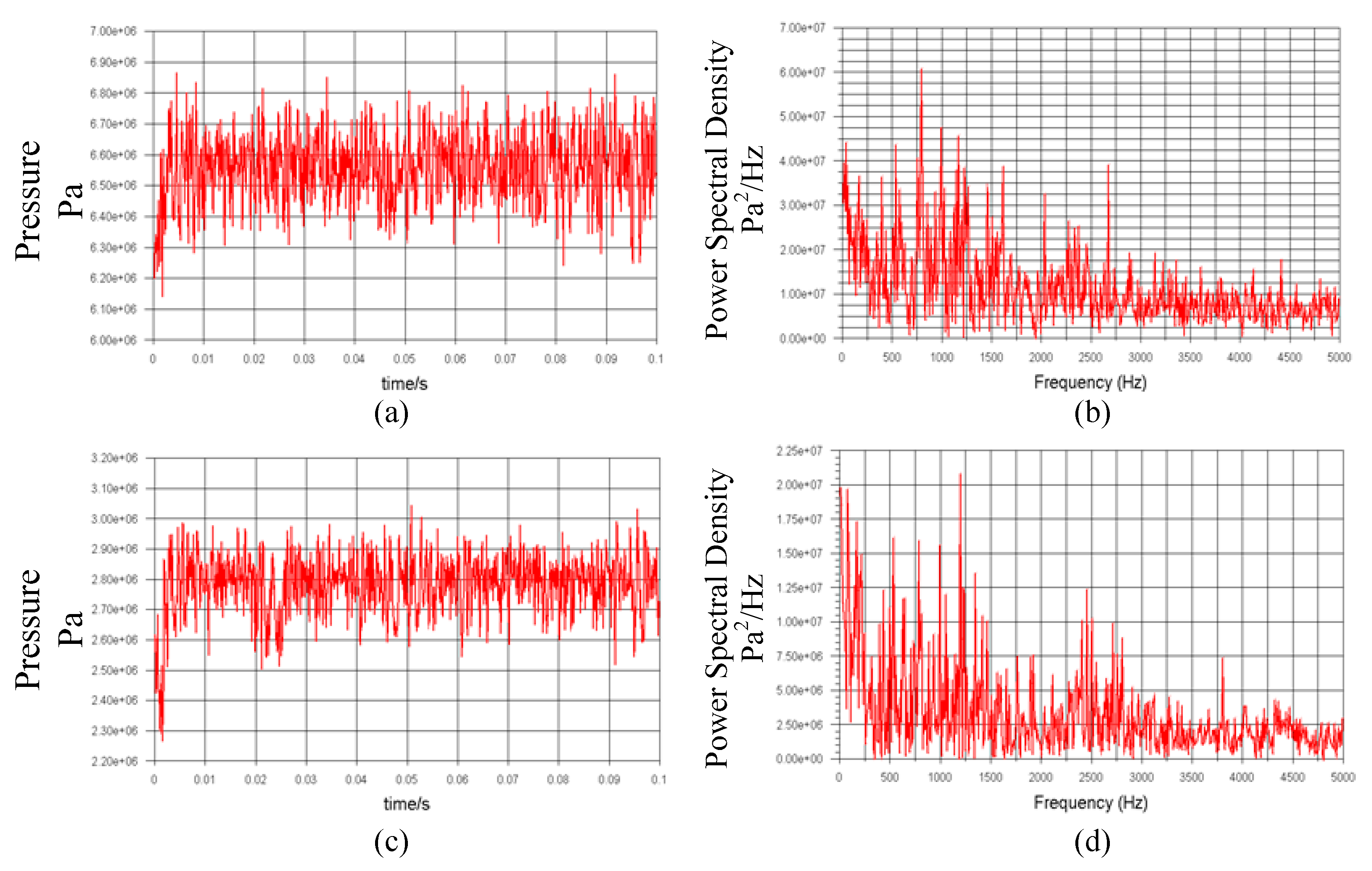
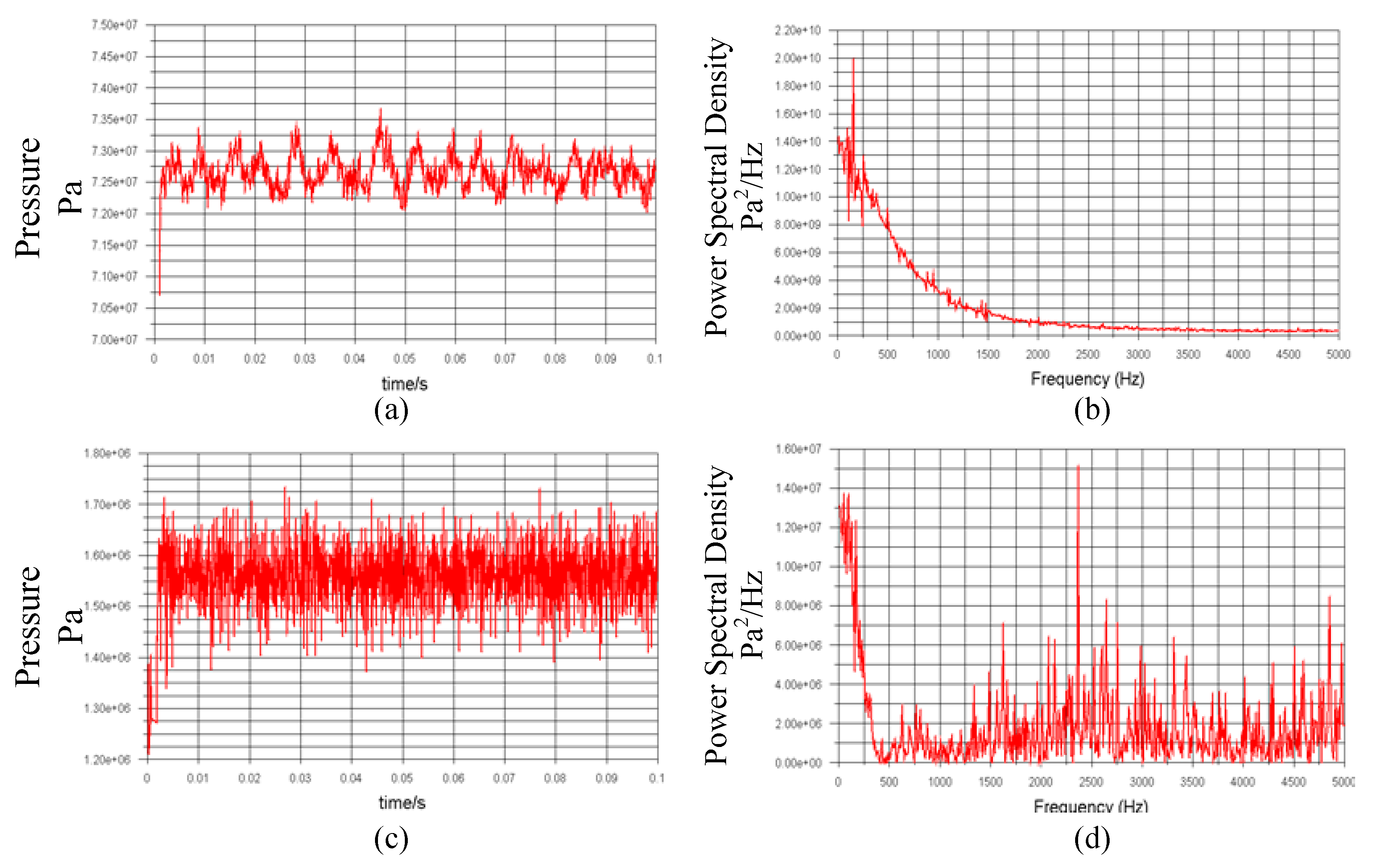
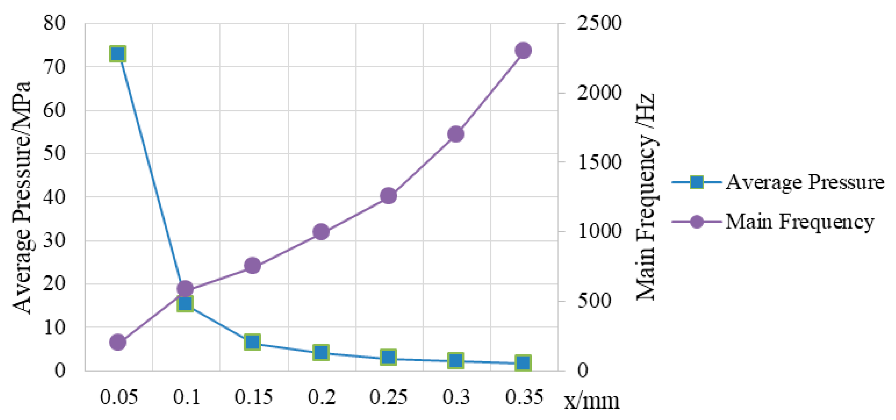
3.3. Variation of Main Frequency and Amplitude of Oscillation under Different Displacements

Under different working conditions, the deflection angle of the flapper of the jet flapper servo valve is different, and the pressure on both sides of the flapper will also be different. Therefore, this section studies the pressure oscillation of the flappers under different displacements while keeping the inlet oil velocity unchanged. When the flapper is at the zero position, the distance between the flapper and the nozzles on both sides is 0.2 mm. The deflection displacement of each flapper is 0.05 mm, and it is in the right direction. Since the distance between the two sides of the flapper is different, the oil flow field on both sides is no longer the same, so in order to compare the pressure difference between the two sides, point 1 and point 2 in Figure 4 are used to observe. Since the flapper at zero point 1 is the same as point 2, only point 1 is selected, as shown in Figure 12, and its pressure oscillates near 0.57 MPa with the main pulsation frequency above 3000 Hz. In Figure 13, Figure 14 and Figure 15, point 1 is closer to the nozzle than point 2, so its overall pressure relative to point 2 is higher, and as can be seen from the spectrum diagram, the pressure of point 1 is also higher. The frequency distribution of the force pulsation is relatively average, but there is a tendency to shift to low, while the pressure of point 2 is mainly high frequency, mainly over 2500 Hz. By analyzing the pressure oscillation curves, the relationship between the force acting on the flapper and the main frequency and the deflection distance of the flapper is obtained as shown in Figure 16. It can be seen that the smaller the distance between the nozzle and the flapper, the stronger the pressure fluctuation, but the relative pressure fluctuation amplitude is positively correlated with the distance as a whole; the main frequency is also related to the distance: the larger the distance is, the greater the main frequency of the pressure oscillation will be. This is because as the distance between the nozzle and the baffle decreases, the fluid resistance of the variable throttle hole increases, the kinetic energy of oil converts into pressure energy increases, and the more hydraulic pressure is generated on the baffle; furthermore, as the distance increases, the greater the turbulence degree of the oil flowing through the nozzle, the greater the pressure oscillation effect of the fluid. This is why the main frequency increases.

3.4. Oscillation Characteristics Considering Motion Coupling of the Main Valve

In this section, the influence of the main valve on the flow field will be considered to establish a more realistic flow field in the servo valve. Similarly, the two-dimensional model is still used in this chapter. The flow field of the whole valve is shown in Figure 17.

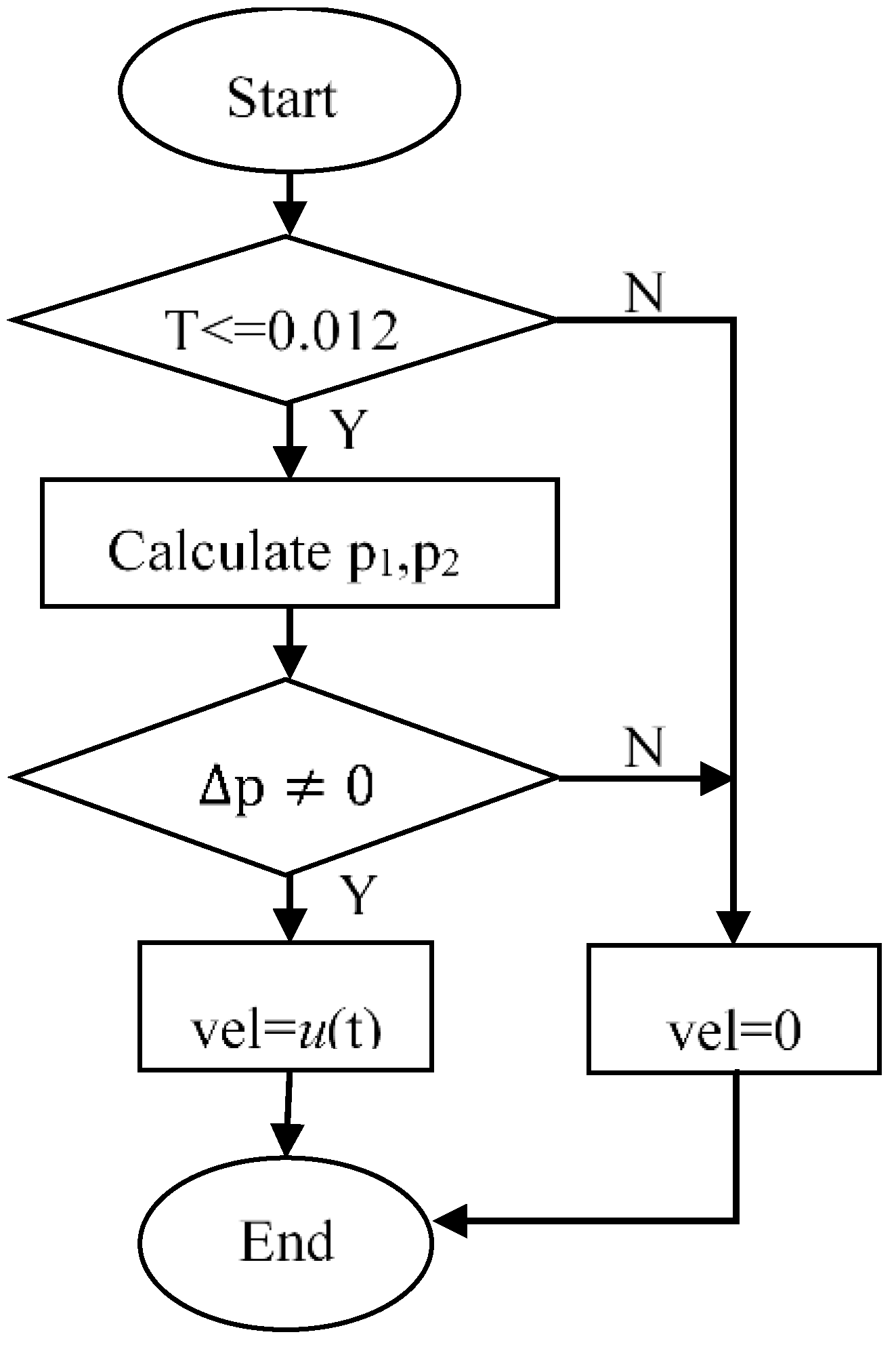
3.4.1. UDF Implementation Logic

During the deflection of the flapper, the displacement of the main valve core will occur with the offset of the flapper. The interface between the valve core and the oil is the moving surface, and the moving distance should be linear with the displacement of the flapper. The moving surface is shown in Figure 18. In order to realize the above moving process, the mathematical model of the main spool motion should be written first.
The main valve mainly plays the role of a power amplifier. The main working process is to move to the side with weak pressure under the pressure difference between the two sides of the pilot valve, so as to realize the opening and closing of the working oil port and realize the function of promoting load movement. In the whole movement process, the main valve is an inlet throttle, which is mainly affected by the steady-state hydrodynamic force, transient hydrodynamic force of opening and closing the working oil outlet, and oil resistance and pressure on both sides of the valve core. Therefore, there is a feedback rod, so there is a feedback force acted by the feedback rod. Its formula is as follows:
m d 2 x ( t ) d t 2 + C f d x ( t ) d t + F R t F R s + F f = A ( p 1 p 2 ) = A Δ p ( t )
where FRt is a transient hydrodynamic force, FRs is a steady hydrodynamic force, and Ff is a feedback force exerted by the feedback rod. Its expressions are shown below and Table 5 shows the meaning and value of each parameter.
F R t = C q 1 w L 3 2 ρ p v d x d t
F R s = 2 C q 1 C v w p v x cos θ
F f = ( r + b ) k f x
By substituting the above formulas and the values of each parameter into Equation (1), the following results are obtained:
d 2 x ( t ) d t 2 + 3010 d x ( t ) d t + 3,566,600 x ( t ) = 3.14 × 10 4 Δ p ( t )
Let u = d x / d t , after Laplacian transformation, obtaining:
U ( s ) s + 3010 U ( s ) + 3,566,600 U ( s ) s = 3.14 × 10 4 Δ P ( s )
U ( s ) Δ P ( s ) = 3.14 × 10 4 s s 2 + 3010 s + 35,666,000
So the velocity curve of the spool in the time domain is:
u ( t ) = 3.14 × 10 4 e 1505 t sin ( 5779 t + 1.32 ) Δ p ( t )
Then, the UDF logic block diagram is written as follows in Figure 18:

3.4.2. Dynamic Grid Design and Simplification for Flapper Deflection

In Section 2.3 we found and validated the reliability of the optimal grid size. Although the flow field of the main valve has been added to this chapter, the final goal of this chapter is to divide the grid model of the whole valve on the basis of the optimal grid size found in the above chapter because the force of the flapper in the nozzle pilot valve area is still the ultimate goal. It has 80,431 grid nodes and 78,741 grid elements. Its element quality, skewness and orthogonal quality are 0.927, 0.032 and 0.994, respectively, which meet the requirements of grid generation. In addition, in order to realize the motion characteristics of the main valve, a moving grid is needed. In this paper, Fluent is used to provide three dynamic grid models: smoothing, layering and regridding. The smoothing model chooses the spring method to smooth the transition; the layering model chooses the height base to set the split factor and collapse factor as default values; and the regridding model chooses the local cell regridding mode, with the maximum surface skewness set to 0.7, and the rest to remain as default.

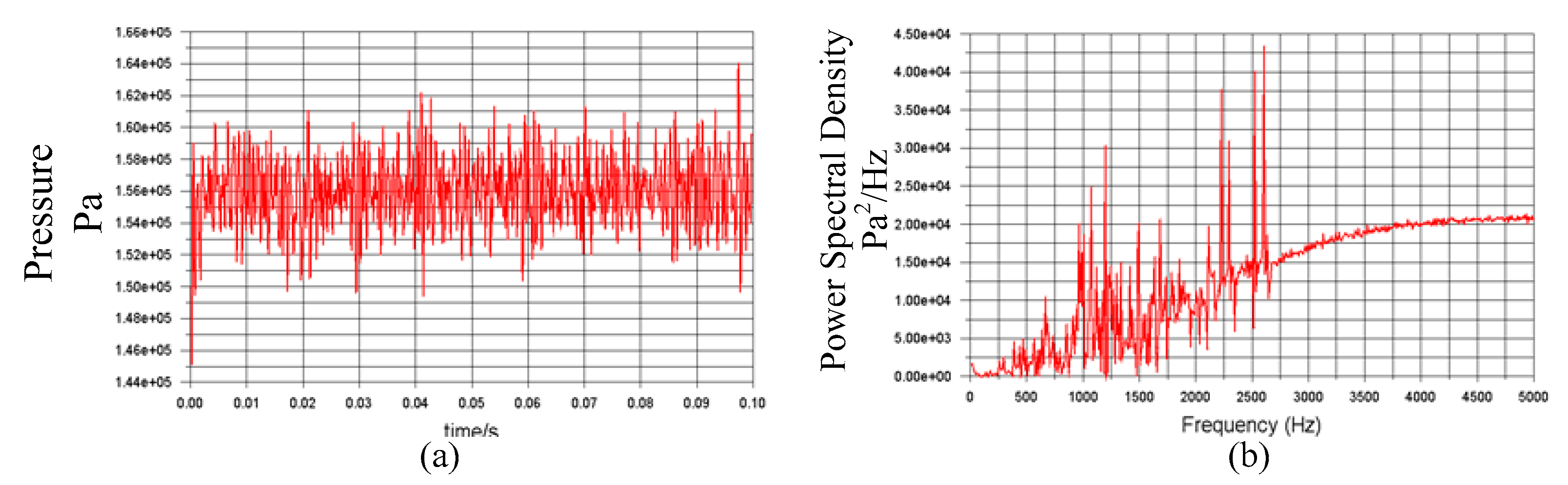
3.4.3. Principal Frequency and Amplitude Change Rule in the Coupling of Main Valve

(1)
Variation of flow field of servo valve with the change of inlet velocity
From Figure 19, Figure 20, Figure 21 and Figure 22, it can be seen that the pressure trend of the flapper is the same as that of the previous one. Figure 23 shows that, with the increase of velocity, the average pressure of the flapper increases and the main frequency decreases, which is the same with the previous one. Unlike the previous one, the relative pressure amplitude does not increase linearly with the speed, but decreases linearly. Moreover, the comparison shows that the peak frequency is also reduced by adding the motion characteristics of the main valve. This is mainly due to the large inertia of the main valve, resulting in its low response frequency. Due to the existence of the feedback rod, this effect is reflected in the flapper, so that the flapper pressure frequency generated by fluid impact is reduced.
(2)
Variation of flow field of the servo valve with the change of the flapper displacement
Points 1 and 2 are taken as monitoring points. When the flapper deflects, the pressure curve of the pilot valve under the influence of the main valve is obtained, as shown in Figure 24, Figure 25, Figure 26 and Figure 27. The pressure under displacement is summarized in Figure 28. The analysis shows that when the distance between the flapper and the nozzle increases, the pressure on the flapper decreases, the relative amplitude increases, and the main frequency increases. The overall trend is consistent with the previous one. It can be seen that the motion characteristics of the main valve do not affect the deflection characteristics of the flapper. At the same time, it can be seen that, whether the main valve exists or not, the pressure level of the pilot valve flapper is not affected at different distances, but the frequency of pressure oscillation is significantly reduced.

4. Conclusions

In this paper, the CFD approach with LES turbulent modeling is utilized for the double flapper nozzle servo valve oscillating flow numerical analysis. The vortex street flow phenomenon could be observed when the flow passes the nozzle flapper channel, the vortex alternating in both sides producing the periodical flow oscillation. With detailed discussion, it could be determined that:
(1) Without the influence of the main valve, the greater the inlet velocity is, the greater the average pressure on the flapper is, and the lower the main frequency of pressure oscillation is.
(2) Without the influence of the main valve, the larger the actual distance between the nozzle and the flapper is, the smaller the average pressure on the flapper is, and the larger the main frequency of pressure oscillation is.
(3) When considering the influence of the main valve, the change trend of hydraulic power and the main frequency of the servo valve flapper are rarely changed, but the main frequency of the pressure oscillation is significantly lower than that without considering the main valve.

Author Contributions

Investigation S.L. and L.L; Simulation and Analysis S.L.; Methodology L.L.; Software S.L.; Writing and Editing S.L., K.Z. and L.L.; Validation L.L. and K.Z.

Funding

The authors are grateful to the National Natural Science Foundation of China (no. 51605333 and no. 51805317) for financial support.

Conflicts of Interest

The authors declare no conflict of interest.

Nomenclature

dInternal diameterDExternal diameter
L1SpacingαAngle
LLengthD1Diameter
L2ThicknessL3Import and Export Center Distance of Load
mSpool masspvPressure difference between inlet and outlet of main valve
xSpool displacementCvOil Flow Velocity Coefficient of Main Valve
CfCoefficient of viscous resistanceθDirectional angle of jet-flow
ASpool end arearDistance between nozzle hole axis and armature Center
p1, p2Pressure at both ends of spoolbAxis pitch from core center to nozzle hole
ρDensity of hydraulic oilKfStiffness of Feedback Bar
Cq1The Flow Coefficient of Main ValveQInlet flow
wArea Gradient of Throttle Hole

References

  1. Jones, J.C. Developments in Design of Electrohydraulic Control Valves; Moog Technical Paper; Moog: Melbourne, VIC, Australia, 1997. [Google Scholar]
  2. Moog, J.W.C. Electrohydraulic Servo Mechanism. U.S. Patent 2,625,136, 13 January 1953. [Google Scholar]
  3. Howard, C.T. Flow Control Servo Valve. U.S. Patent 2,790,427, 30 April 1957. [Google Scholar]
  4. Atchley, R.D. Valve. U.S. Patent 3,017,864, 23 January 1962. [Google Scholar]
  5. Vanderlaan, R.D.; Meulendyk, J.W. Direct Drive Valve-Ball Drive Mechanism. U.S. Patent 4,672,992, 16 June 1987. [Google Scholar]
  6. Laux, K. Motor-to-Spool Coupling for Rotary-to-Linear Direct Drive Valve. U.S. Patent 5,263,680, 23 November 1993. [Google Scholar]
  7. Samakwong, T.; Assawinchaichote, W. PID controller design for electro-hydraulic servo valve system with genetic algorithm. Procedia Comput. Sci. 2016, 86, 91–94. [Google Scholar] [CrossRef]
  8. Brito, A.G.; Leite, F.W.C.; Hemerly, E.M. Identification of a Hammerstein model for an aerospace electrohydraulic servovalve. IFAC Proc. Vol. 2013, 46, 459–463. [Google Scholar] [CrossRef]
  9. Khodaee, Z.; Zareinejad, M.; Ghidary, S.S. Modeling of a two-stage flapper-nozzle electrohydraulic servo valve exposed to acceleration. In Proceedings of the 2014 Second RSI/ISM International Conference on Robotics and Mechatronics (ICRoM) IEEE, Tehran, Iran, 15–17 October 2014; pp. 268–273. [Google Scholar]
  10. Ye, S.; Zhang, J.; Xu, B.; Zhu, S.; Xiang, J.; Tang, H. Theoretical investigation of the contributions of the excitation forces to the vibration of an axial piston pump. Mech. Syst. Signal Process. 2019, 129, 201–217. [Google Scholar] [CrossRef]
  11. Li, S.; Aung, N.Z.; Zhang, S.; Cao, J.; Xue, X. Experimental and numerical investigation of cavitation phenomenon in flapper–nozzle pilot stage of an electrohydraulic servo-valve. Comput. Fluids 2013, 88, 590–598. [Google Scholar] [CrossRef]
  12. Chen, M.; Aung, N.Z.; Li, S.; Zou, C. Effect of oil viscosity on self-excited noise production inside the pilot stage of a two-stage electrohydraulic servovalve. J. Fluids Eng. 2019, 141, 011106. [Google Scholar] [CrossRef]
  13. Qian, J.Y.; Chen, M.R.; Liu, X.L.; Jin, Z.J. A numerical investigation of the flow of nanofluids through a micro Tesla valve. J. Zhejiang Univ. Sci. A 2019, 20, 50–60. [Google Scholar] [CrossRef]
  14. Chao, Q.; Zhang, J.; Xu, B.; Huang, H.; Zhai, J. Effects of inclined cylinder ports on gaseous cavitation of high-speed electro-hydrostatic actuator pumps: A numerical study. Eng. Appl. Comput. Fluid Mech. 2019, 13, 245–253. [Google Scholar] [CrossRef]
  15. Qian, J.Y.; Gao, Z.X.; Liu, B.Z.; Jin, Z.J. Parametric study on fluid dynamics of pilot-control angle globe valve. J. Fluids Eng. 2018, 140, 111103. [Google Scholar] [CrossRef]
  16. Zhang, J.H.; Wang, D.; Xu, B.; Gan, M.Y.; Pan, M.; Yang, H.Y. Experimental and numerical investigation of flow forces in a seat valve using a damping sleeve with orifices. J. Zhejiang Univ. Sci. A 2018, 19, 417–430. [Google Scholar] [CrossRef]
  17. Yin, Y.B. Theory and Application of Advanced Hydraulic Component; Shanghai Scientific & Technical Publishers: Shanghai, China, 2017. [Google Scholar]
  18. Wang, F.J. Computational Fluid Dynamics Analysis; Tsinghua University Press: Beijing, China, 2004. [Google Scholar]
Figure 1. Principle diagram of jet flapper valve. (a) Structure schematic diagram of servo valve. (b) Pre-stage flow field and boundary conditions.
Processes 07 00721 g001
Figure 2. Grid model with a grid size of 0.012 and the flapper at the zero position when L1 = 0.02.
Processes 07 00721 g002
Figure 3. Flow and pressure at different grid sizes.
Processes 07 00721 g003
Figure 4. Nozzle structure with observation points and the Y plus distribution. (a) Nozzle structure with observation points. (b) The Y plus distribution when velocity of inlet is 10 m/s.
Processes 07 00721 g004
Figure 5. Velocity nephogram in one oscillating period.
Processes 07 00721 g005
Figure 6. Pressure oscillation curves at different points on flappers. (a) Point 1 in the time domain. (b) Point 1 in the frequency domain. (c) Point 2 in the time domain. (d) Point 2 in the frequency domain. (e) Point 3 in the time domain. (f) Point 3 in the frequency domain. (g) Point 5 in the time domain. (h) Point 5 in the frequency domain.
Processes 07 00721 g006
Figure 7. Pressure curves in time and frequency domains when the inlet velocity is 5 m/s. (a) Time domain. (b) Frequency domain. (c) 20logE frequency domain.
Processes 07 00721 g007
Figure 8. Pressure curves in time and frequency domains when the inlet velocity is 10 m/s. (a) Time domain. (b) Frequency domain. (c) 20logE frequency domain.
Processes 07 00721 g008
Figure 9. Pressure curves in time and frequency domains when the inlet velocity is 25 m/s. (a) Time domain. (b) Frequency domain. (c) 20logE frequency domain.
Processes 07 00721 g009
Figure 10. Pressure curves in time and frequency domains when the inlet velocity is 50 m/s. (a) Time domain. (b) Frequency domain. (c) 20logE frequency domain.
Processes 07 00721 g010
Figure 11. Pressure oscillation and main frequency of the flappers at different velocities.
Processes 07 00721 g011
Figure 12. Pressure oscillation curve of the flapper when the displacement of the flapper is x = 0.00 mm. (a) Point 1 in the time domain. (b) Point 1 in the frequency domain.
Processes 07 00721 g012
Figure 13. Pressure oscillation curve of the flapper when the displacement of the flapper is x = 0.05 mm. (a) Point 1 in the time domain. (b) Point 1 in the frequency domain. (c) Point 2 in the time domain. (d) Point 2 in the frequency domain.
Processes 07 00721 g013
Figure 14. Pressure oscillation curve of the flapper when the displacement of the flapper is x = 0.10 mm. (a) Point 1 in the time domain. (b) Point 1 in the frequency domain. (c) Point 2 in the time domain. (d) Point 2 in the frequency domain.
Processes 07 00721 g014
Figure 15. Pressure oscillation curve of the flapper when the displacement of the flapper is x = 0.15 mm. (a) Point 1 in the time domain. (b) Point 1 in the frequency domain. (c) Point 2 in the time domain. (d) Point 2 in the frequency domain.
Processes 07 00721 g015
Figure 16. Average pressure and main frequency of the flapper at different actual distances between the nozzle and flapper.
Processes 07 00721 g016
Figure 17. Watershed model of the servo valve considering the effect of the main valve.
Processes 07 00721 g017
Figure 18. Execution logic block diagram of UDF program (the symbol T means time, and the value 0.012 is the time of the moving grid motion).
Processes 07 00721 g018
Figure 19. Pressure oscillation curve of the flapper considering the impression of the main valve and velocity of 5 m/s. (a) Time domain. (b) Frequency domain.
Processes 07 00721 g019
Figure 20. Pressure oscillation curve of the flapper considering the impression of the main valve and velocity of 10 m/s. (a) Time domain. (b) Frequency domain.
Processes 07 00721 g020
Figure 21. Pressure oscillation curve of the flapper considering the impression of the main valve and velocity of 25 m/s. (a) Time domain. (b) Frequency domain.
Processes 07 00721 g021
Figure 22. Pressure oscillation curve of the flapper considering the impression of the main valve and velocity of 50 m/s. (a) Time domain. (b) Frequency domain.
Processes 07 00721 g022
Figure 23. Pressure and main frequency of the servo valve flapper at different speeds.
Processes 07 00721 g023
Figure 24. Pressure oscillation curve of the flapper under the influence of the main valve when the displacement of the flapper is x = 0.00 mm. (a) Point 1 in the time domain. (b) Point 1 in the frequency domain.
Processes 07 00721 g024
Figure 25. Pressure oscillation curve of the flapper under the influence of the main valve when the displacement of the flapper is x = 0.05 mm. (a) Point 1 in the time domain. (b) Point 1 in the frequency domain. (c) Point 2 in the time domain. (d) Point 2 in the frequency domain.
Processes 07 00721 g025
Figure 26. Pressure oscillation curve of the flapper under the influence of the main valve when the displacement of the flapper is x = 0.10 mm. (a) Point 1 in the time domain. (b) Point 1 in the frequency domain. (c) Point 2 in the time domain. (d) Point 2 in the frequency domain.
Processes 07 00721 g026
Figure 27. Pressure oscillation curve of the flapper under the influence of the main valve when the displacement of the flapper is x = 0.15 mm. (a) Point 1 in the time domain. (b) Point 1 in the frequency domain. (c) Point 2 in the time domain. (d) Point 2 in the frequency domain.
Processes 07 00721 g027
Figure 28. Pressure and main frequency of the flapper when the actual distance between the flapper and nozzle changes.
Processes 07 00721 g028
Table 1. Nozzle parameters of the flapper nozzle valve.
ParameterNumerical Value
Reference pressure/MPa0.1
Density/kg∙m−3889
Dynamic Viscosity/Pa·s0.04
Modulus of elasticity/MPa1000
NozzleInternal diameter/d0.5
External diameter/D1
Spacing/L10.2
Length/L1.0
Angle/α30
FlapperDiameter/D12.0
Thickness/L21.5
Table 2. Solution strategy.
Emulation ItemsEmulation Settings
Fluid stateSingle-phase turbulent transient
Pressure algorithmSIMPLEC
Discrete schemeSecond-order upwind
Pressure correction algorithmPRESTO!
Transient equationSecond-order implicit equation
Simulation step size0.0001s
Table 3. Grid parameters.
Grid Size/mmNodesElementsElement QualitySkewnessSkewness
(max)
Orthogonal QualityOrthogonal Quality
(min)
0.01026,09025,4110.8350.0780.6430.9820.544
0.01222,79522,1500.8390.0680.6090.9850.544
0.01520,04819,4400.8390.0660.7590.9850.312
0.02017,81517,2430.8410.0660.7880.9850.272
Table 4. Grid model parameters of different spacing between nozzle and flapper.
Flapper Displacement x/mmNodesElementsElement QualitySkewnessSkewness
(max)
Orthogonal Quality
x = 0.0022,79522,1500.8390.0680.6090.985
x = 0.0520,92220,2910.8990.0710.6690.986
x = 0.1022,95322,2920.8360.0690.7470.983
x = 0.1520,96720,3210.9090.0610.6760.989
Table 5. Parameters for mathematical modeling of servo valves.
ParameterValueParameterValue
Spool mass m/kg0.01Import and Export Center Distance of Load L3/m1.34 × 10−2
Spool displacement x/m Pressure difference between inlet and outlet of main valve pv/MPa5
Coefficient of viscous resistance Cf/kg·s−117.4Oil Flow Velocity Coefficient of Main Valve Cv0.99
Spool end area 3.14 × 10⁻⁶Directional angle of jet-flow θ69
Pressure at both ends of spool p1, p2 Distance between nozzle hole axis and armature Center r/m2.0 × 10−3
Density of hydraulic oil ρ/kg·m−3889Axis pitch from core center to nozzle hole b/m3.0 × 10−3
The Flow coefficient of the main valve Cq10.8Stiffness of Feedback Bar kf/N·m−13.4 × 103
Area gradient of the throttle hole w/m21.256 × 10−2Inlet flow Q/m3·s−18.3 × 10−5

