1. Introduction
The fire flooding experiment launched in DU Block 66 of Liaohe Oilfield ended with a great success. As the fire flooding continuously deepens, more vapor and solution gas will be produced in bushings of producing wells. As a result, internal walls of separators at sulphur removal stations are badly eroded, followed by the desulfurizing agent getting hydrolyzed and losing its efficacy, the gas–liquid separator showing a lower efficiency, and so on.
The gas intake of the separator studied in this paper fluctuates between 60,000 m3 and 150,000 m3 per day. Based on the constituents (CH4, CO2, N2, H2S, O2) of the tail gas collected from the oilfield, the contents of CO2, N2, CH4, O2 and H2S are between 3–30%, 20–80%, 10–75%, 0–3% and 0–0.0004%, respectively. So, the liquid phase of the tail gas could be considered as a Newtonian fluid. Moreover, since the operating pressure of the gas–liquid separator is 0.05 MPa (manometer pressure), the gas phase could be considered as an incompressible fluid when simulated.
Nowadays, viscous oil fire flooding has been a new technology with rapid development, while tail gas disposing could be an important link for production safety [
1,
2]. A gas–liquid separator is used to remove water droplets contained in tail gas. Many scholars used a
k-
ε model to study the separation efficiency of particles within the separator [
3,
4,
5], thus obtaining the particle separation efficiency under different operating conditions; however, the research of numerically stimulating gas–liquid double-phase flow is not very common. The internal structure of a gas–liquid separator is complex and there are many factors affecting the effect of gas–liquid separation, leading to the difficulty for calculation. Up until now, the research is still imperfect [
6]. In this regard, the process of gas–liquid separating inside the equipment is simulated based on actual producing data of the oil field. This can show clearly how the separator operates, and is of important significance in setting up reasonable working conditions of separator parameters, thereby improving the separation efficiency [
7].
In this research, the Fluent software is adopted to construct a numerical model of the separator, and thus to stimulate the process of gas–liquid separating inside the equipment. The results of the calculations turn out to be identical to that from the oil field. On this basis, the separation efficiency is obtained through calculation under different inlet water contents and inlet velocities. Combined with the separator’s internal flow field distribution, it may assist in confirming how different inlet water contents and inlet velocities influence the separation efficiency, and eventually optimize the structure of the separator based on the calculation results [
8].
2. Description of Models
The fluid may be impacted by three basic laws of physics, namely the mass conservation, the momentum conservation and the energy conservation. The differential form of the three equations is also called the constitutive equation. This paper is mainly used to simulate the gas–liquid separation efficiency under constant temperature. Therefore, only with the mass conservation and the momentum conservation equations considered, this paper is simulating the flow field and flow regime where an RNG k-ε (renormalization group techniques, turbulent energy k and dissipation rate ε) model is employed, and using the RNG method on an N-Sequation (Navier-Stokes equation), getting an RNG-based governing equation.
The continuity and momentum equations are expressed as Equations (1) and (2).
The RNG
k-
ε equation is expressed as Equations (4) and (5),
where
u is the velocity,
p is the pressure,
ρ is the density,
ν is the coefficient of viscosity,
ν =
ν0 +
νt,
ν0 is the kinematic viscosity,
νt is the eddy viscosity,
δij is the Kronecker delta,
k is the specific turbulent kinetic energy,
ε is the turbulent dissipation rate,
R is the additional term,
η is the ratio of the turbulent time scale to the mean strain scale,
η0 is the typical numerical of
η in uniform shear flow,
η0 = 4.38,
c1 = 1.42,
c2 = 1.68,
αk =
αε = 1.39,
cμ = 0.0845, and
β = 0.012.
As a kind of simplified multiphase flow model, the mixture model applies the basic approach of a single-phase fluid by simulating multiphase flows with various velocities, but it assumes that a local balance has been achieved on a short spatial scale with a strong coupling relation. The mixture model can be used in simulating multiphase flows through solving the momentum, continuity and energy equations on a mixed phase, the second-phase volume fraction equation, and the relative velocity equation.
The continuity equation for this mixture is expressed as Equation (8).
Here,
ml,
Vl and
ρl are the mass, volume and density of the liquid phase, respectively, and
g is the gravitational acceleration.
ul and
ug represent the velocity fields for the liquid phase and the gas phase, respectively. The subscript
m refers to the mass-averaged variables (properties) of the mixture. Defining the volume fraction of the liquid phase as α
l =
Vl/Vm and α
g = 1 − α
l, with the mass fraction of the liquid phase defined as
cl = α
lρl/
ρm, the mass-averaged velocity and the mixture density can be defined, respectively, as:
The momentum conservation equation for the mixture is expressed as Equation (10).
In this equation, the momentum transfer between the phases is accounted for by the third term on the right-hand side. This term represents the momentum diffusion due to the relative motion, or, as we are referring to it in our analysis, the diffusive flux due to phase slip; and the diffusion (drift) velocities are defined for gas and liquid phases, respectively, as
uml =
ul − um, and
umg =
ug − um. The volume fraction of liquid phases can be presented as:
The model is accurate only when the response (relaxation time) for reaching an equilibrium slip velocity between the dispersed phases and the host fluid is very short. Numerically, this means that the dispersed phase reaches a constant terminal velocity over a spatial length that is smaller than that of the computational cell.
3. Model Construction and Mapped Meshing
In practical production, the flow regime of the fluid in the equipment is mostly in turbulent hydraulic smooth area, so the turbulence pattern theory is mainly adopted. In the Fluent software, the k-ε model, Spalart–Allmaras model, k-ω model and Reynolds stress model (RSM) all belong to the turbulence pattern theory. We researched five turbulence models:
- (1)
Standard k-ε model: This model, put forward by Launder and Spalding, is widely used for industrial flow field, heat transfer simulation, and so on, and is reasonable in economy and precision.
- (2)
RNG k-ε model: This model from strict statistical algorithms may help improving precision (especially in the area of turbulent eddies); besides, it takes the low-Reynolds-number flow viscosity analytical formula into consideration.
- (3)
Swirling modification k-ε model: This model adds a new formula for turbulent viscosity and a new transmission equation for dissipation rating.
- (4)
Standard k-ω model: This model takes the low Reynolds number, compressibility and shear flow into account.
- (5)
SST k-ω model (Menter’s shear stress transport k-ω model): This model merges the cross diffusion derived from the equation of omega and it includes the spread of turbulent shear stress.
In terms of computation, an RNG
k-
ε model tends to cost more computer resources than a standard
k-
ε model does; the former is specially designed to deal with a lower turbulent viscosity caused by high tension, with the turbulent eddy taken into consideration, compared with the standard
k-
ε model, and thus has a better performance in strong streamline flex, eddy and rotating simulation. It is considered that the RNG
k-
ε model can be applied to viscous flow with relatively low Reynolds number. Thanks to those features, the RNG
k-
ε model represents a higher credibility and accuracy than the standard
k-
ε model in a wider flow. Comparing the differences in calculation precision and computing time, it can be summarized that the RNG
k-
ε is most suitable for simulation [
9,
10,
11].
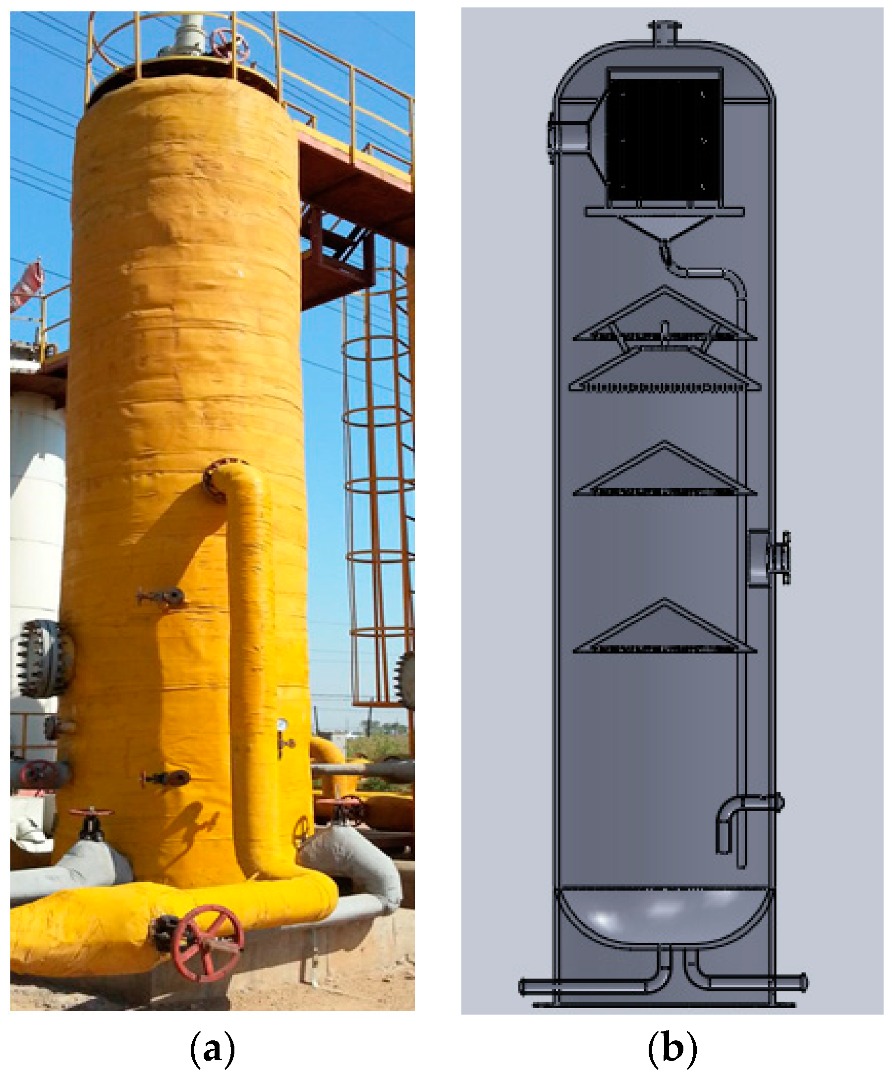
As shown in
Figure 1,
Figure 1b is the 3D model constructed by SolidWorks based on the structure parameters of the equipment (a) in the oil field. As some parts of the structure have no impact on the gas–liquid separation effect, we should simplify the model of the separator and then mesh the model with ICEM CFD (integrated computer rngineering and manufacturing code for computational fluid dynamics) [
12,
13].
The separator is 7345 mm high, with body length of 6000 mm, outside diameter of 1664 mm, and wall thickness of 42 mm. The assembly model of the cyclone separator consists of 17 parts.
The boundary conditions of the model are set as follows:
- (1)
Separator inlet boundary condition: As for continuous phase (gas), set the gas inlet flow rate to be vertical with separator’s inlet cross-section; as for dispersed phase (liquid drop), set the liquid drop to be evenly distributed on the inlet cross-section, refer to the drop settling speed specified by the separator for the inlet speed of drop, and take the working pressure of the separator as the operating pressure.
- (2)
Separator’s outlet boundary condition: Dispose according to artesian outlet for gas–liquid two-phase.
- (3)
Wall condition of separator: Wall boundary conditions of vertical-type gas–liquid separators mainly include a corrugated plate, umbrella cap separator and inner wall, separately giving the boundary conditions based on the simulation process; as for the dispersed phase, set boundary conditions as reflection, escape and gathering for dispersed phase (see
Table 1 for specific inlet and outlet parameter settings). Mesh the model of the gas–liquid separator, with 3,843,940 nodes and 22,848,895 grids, whose quality is above 0.35. Computational fluid dynamics (CFD) has many requirements for grid computing, including smoothness, orthogonality and amount of grid nodes in areas with dramatic changes in flowing. The separator studied in this paper is geometrically complicated and giant in volume, with a grid quality of 0.35 in the orthogonal computation under boundary conditions of the object. For relatively large models, the computational grid quality suggested by Fluent is over 0.3. Through repeated trials, outputs of the models with grid quality of 0.35 are in good conformity with the results actually measured by the separator, and therefore, through the grid division shown in this paper, we can find the complex flow characteristics for further computation and analysis. This matches with the requirement for calculation, and can be imported into Fluent for numerical calculation.
The computational accuracy and error in different grid divisions can reflect to what degree the data computed by employing such models matches with and deviates from the real physical field. The outlet fluid velocity can reflect, in different grid divisions, to what degree the computational result is similar to the real physical field, that is, the degree of accuracy, while the outlet moisture content can reflect the dehumidification efficiency of the separator under the foresaid computational model, which will be compared with the practical data for an error analysis. Hence, we employ the outlet fluid velocity and the moisture content to embody the computational accuracy and error in different models, where the computational accuracy is the ratio of calculated outlet fluid velocity to practical value, the error is the ratio of calculated outlet moisture content to practical value, both are dimensionless and 1 is the optimal value. We can check if a grid division is rational by comparing the outlet fluid velocity in different models, while the outlet moisture content can reflect to what degree a computational model deviates from the onsite actual data.
The separator grid type consists of structured and unstructured grids. The mesh and the numerical simulation validation are shown in
Figure 2 and
Table 1, respectively. During computation, the coarsened grid model of case 1 shows a less smooth transition, discontinuous computation, ending with an outlet flow velocity dramatically different from actual velocity, which fails to conform to the onsite law. Hence, although it takes the shortest time to compute, such grid division is still dismissed. Based on the precision and the actual scene, we prefer case 2.
There are four types of commonly used models of multiphase flow, the VOF (volume of fluid) model, the mixture model, the Eulerian model and the level set (LS) method. The LS method is implemented by means of user-defined functions (UDFs), and it is coupled to the Fluent built-in VOF to capture the interface between two immiscible fluids.
In LS methods, the interface is represented by zero contour of a continuously signed distance function; this is known as the level set function. The movement of the interface is governed by a transport equation supporting the level set function. To keep the level set function as a signed distance function, a re-initialization process is needed. LS methods automatically deal with topological changes. It is generally easy to obtain a high order of accuracy just by using an ENO (essentially non-oscillatory) or WENO (weighted essentially non-oscillatory) scheme. However, LS methods are not conservative, so that a significant, physically incorrect loss or gain of mass occurs in the case of incompressible two-phase flow. Several authors have overcome this problem by coupling the LS and VOF methods. In such coupled level set volume of fluid (CLSVOF) techniques, the level set function is used to accurately compute the curvature and the normal to the interface, while the volume of fluid function is used to capture the interface. Normally, a CLSVOF method is more accurate than both the LS and VOF methods alone.
In this paper, our goal of simulation is the liquid and gas volume at the outlet of the separator, instead of the gas–liquid two-phase separation details in the internal separator. To avoid complicated coupled methods, we choose the VOF model, the mixture model and the Eulerian model.
Among them, the VOF model is better at reflecting the interface conditions between multiphase flows; for example, the gas–liquid interface with large bubbles flowing in liquid at relatively slow speeds, and so on, since the physical parameters in the equations used in the VOF model are the volume averages of the physical properties of each phase. Therefore, it is required that the difference between the speeds of the phases should not be too large, otherwise it will have a great impact on the accuracy of the calculation results. In general, VOF is adopted with better performance in non-steady state simulation.
The mixture and Eulerian models are suitable for mixing or separation flow, and when discrete phase volume share is more than 10%. In the computational domain, when discrete phase distribution is wild, the mixture model is recommended instead of the Eulerian model.
Considering the establishment of the numerical simulation model and the calculation of the dehumidification equipment discrete items, we choose the mixture model.
4. Calculation Parameter Setting
The mixture multiphase flow model is adopted to stimulate the process of gas and liquid separating. Gas- and liquid-phase mixture flows in the separator through the entrance of the equipment. The second-order upwind difference scheme is adopted for the convection item and the diffusion term in the equation, while the SIMPLEC (semi-implicit method for pressure linked equations-consistent) algorithm is used for the continuity equation and the momentum equation.
The model with mesh generated is imported into Fluent, the model under normal operation conditions is simulated, and then the result with the dew-point instrument from the field is tested; calculation parameters for the vertical separator model are shown in
Table 2 below.
During modeling, the ICEM (integrated computer engineering and manufacturing code) software is used to optimize the grid model; not only the near-surface grid is refined, but the near-wall region is also optimized from being dense to being coarse; under the RNG k-ε model, the finally measured grid parameter y+ = 35.
By converting the flowrate on the basis of the Clapyron equation, the velocity of flow is obtained under operating conditions of 15.55 m/s. Since it is impossible to achieve a result in conformity with practical onsite data through one numerical simulation only, the model has been approximated, adjusted and optimized a lot on grid division, equation discrete schemes, spacing and convergence requirements based on actual data and the gas-phase moisture content we computed by usage of the data collected from the outlet under current working conditions.
5. Analyzing Influence Factors of Dehumidification Efficiency
The moisture content calculated by the model is 178.34 ppm. After adjusting the model by modifying the boundary conditions, we calculate that the moisture content is 179.8 ppm. Compared with the actual moisture content, the percentage of error is within 0.72%. Based on the result, we further study the influence factors of dehumidification efficiency.
Importing the model which is meshed into grids into Fluent, inlet water volume percentages of 100 ppm, 216 ppm, 400 ppm and 600 ppm are taken in for calculation, the inlet pressure is 0.05 MPa, the rates of flow are 15 m/s, 20 m/s, 25 m/s and 30 m/s, and the corresponding rates of flow are 83,784 m3/d, 111,712 m3/d, 139,640 m3/d and 167,568 m3/d. We are studying the fluid velocity distribution inside the equipment under different moistures and entrance velocities as follows:
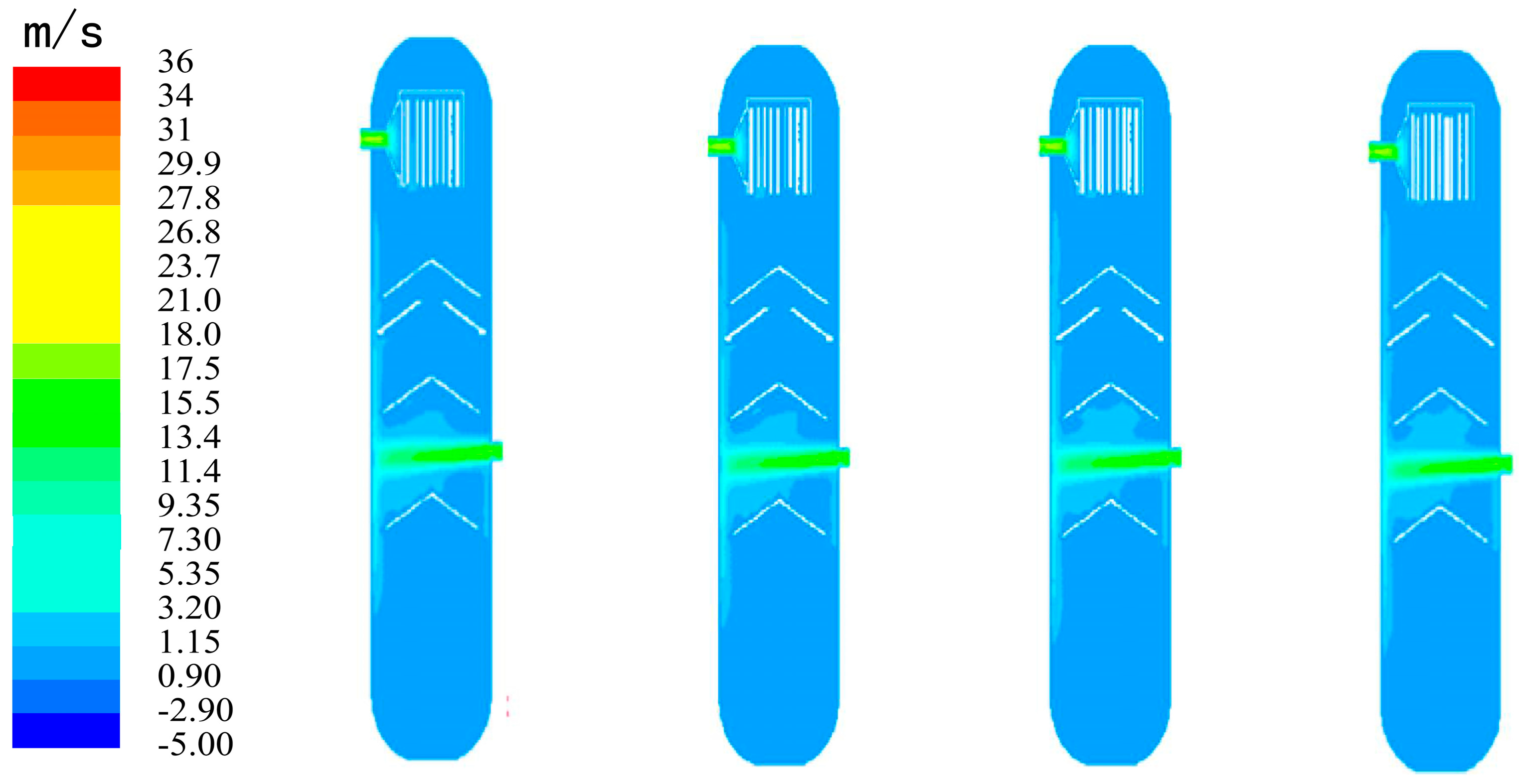
(1) The influence of different water contents on velocity distribution
Figure 3 displays the velocity distribution within the equipment when the entrance is with a flow rate of 15 m/s, while the entrance moisture content from left to right is 100 ppm, 216 ppm, 400 ppm and 600 ppm. As shown in the figure, the fluid under a certain velocity is able to spread to the separating umbrella of the preliminary separation zone in a high velocity, and the zone can be taken full use of. Nevertheless, when the fluid enters the equipment, it hits the wall first. The fluid with high velocity flows over the preliminary separation zone and flows directly to the corrugated plate in the fine separation zone.
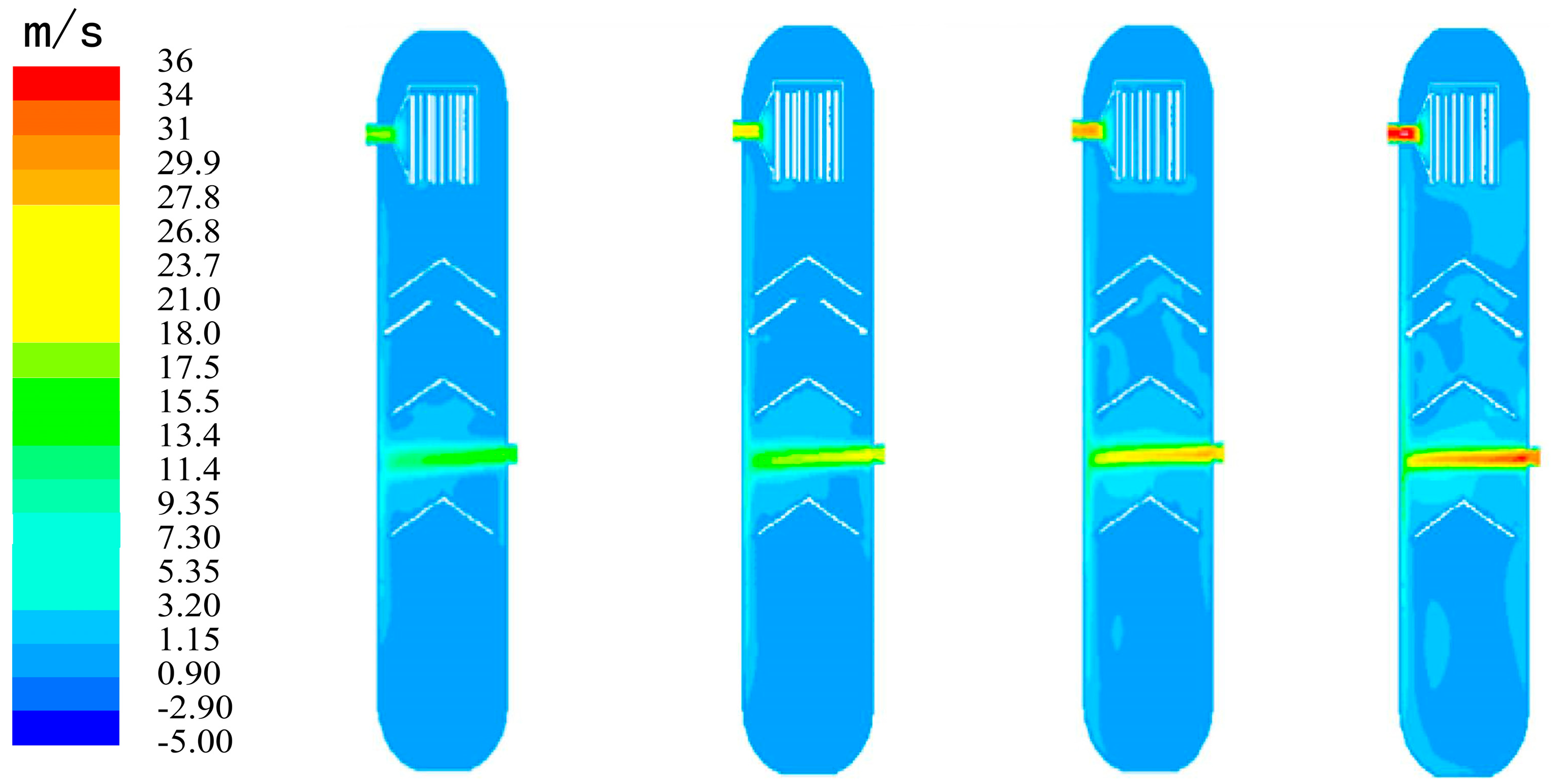
(2) The influence of different entrance velocities on velocity distribution
As it is shown in
Figure 4, and with the velocity increased, the flow velocity of export increases obviously. From the decreasing trend of the gas in the figure we can see that the gas moves along the wall of the separator within the range of the flow velocity. When the velocity is low, the speed of gas passing the corrugated plate is low, and most of the moisture flows directly to the fine separation zone rather than to the preliminary separation zone. From the velocity distribution in the figure, we can conclude that high velocity is conductive to the movement of the gas inside the separator, and the moisture can be fully touching the separating umbrellas in the preliminary separation zone and fine separation zone. By increasing the separation efficiency, the load of the fine separation zone can be reduced.
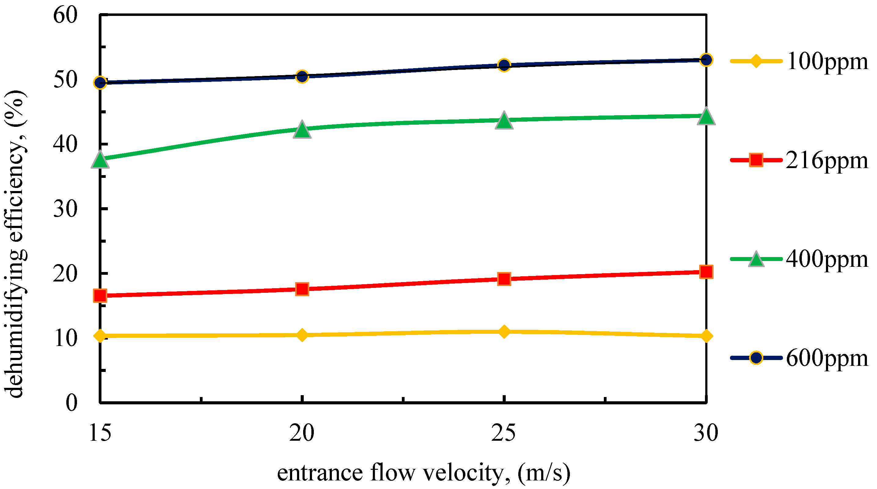
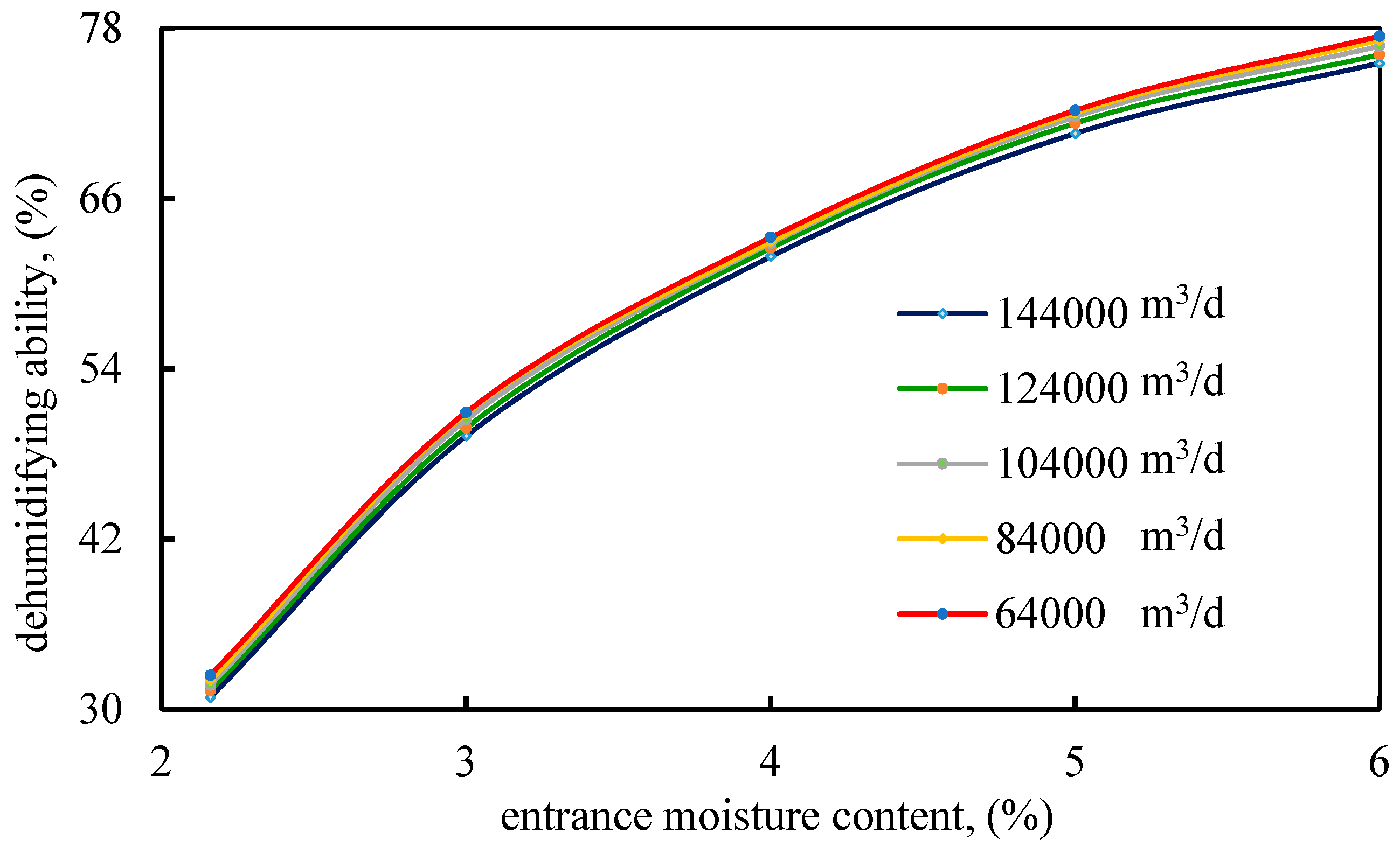
At last, through comparison among various export water volume percentages, the dehumidifying ability of the separator is determined in this paper. The calculating result is shown in
Figure 5. The dehumidification efficiency equals the ratio of inlet moisture content minus the ratio of outlet moisture content, then divided by the ratio of inlet moisture content.
As it is shown in
Figure 5, under the same entrance flow velocity and within the entrance moisture content range of 600 ppm, the dehumidification efficiency increases with the initial water volume percentage increasing, meaning that the equipment cannot reach the maximum ideal load value and the variation range of dehumidification efficiency is not obvious. From all these factors above, it can be seen that when the entrance velocity is within the range of 30 m/s, dehumidification efficiency is mainly related to the value of the inlet water volume percentage.
6. Optimizing the Structure of the Separator
During the simulation, we have found that the velocity of tail gas during the separation is too high, leading the gas to impose a high-speed impact on the wall, as it is shown in
Figure 6. Meanwhile, due to the low pressure in the operating conditions, the flow velocity of the fluid is larger in the preliminary separation zone. This leads to the umbrella being unable to play a role well; in addition, the velocity of fluid flowing through the fine separation of the corrugated plate is also bigger, the contact time is shorter, the liquid phase in the flowing space has no time to collide, coalesce and separate from corrugated plate, and the separation efficiency has been seriously affected. In the case where this condition continues for a long time, the gas will corrode the wall inside the equipment; as a consequence, it is necessary to optimize the structure of the separator.
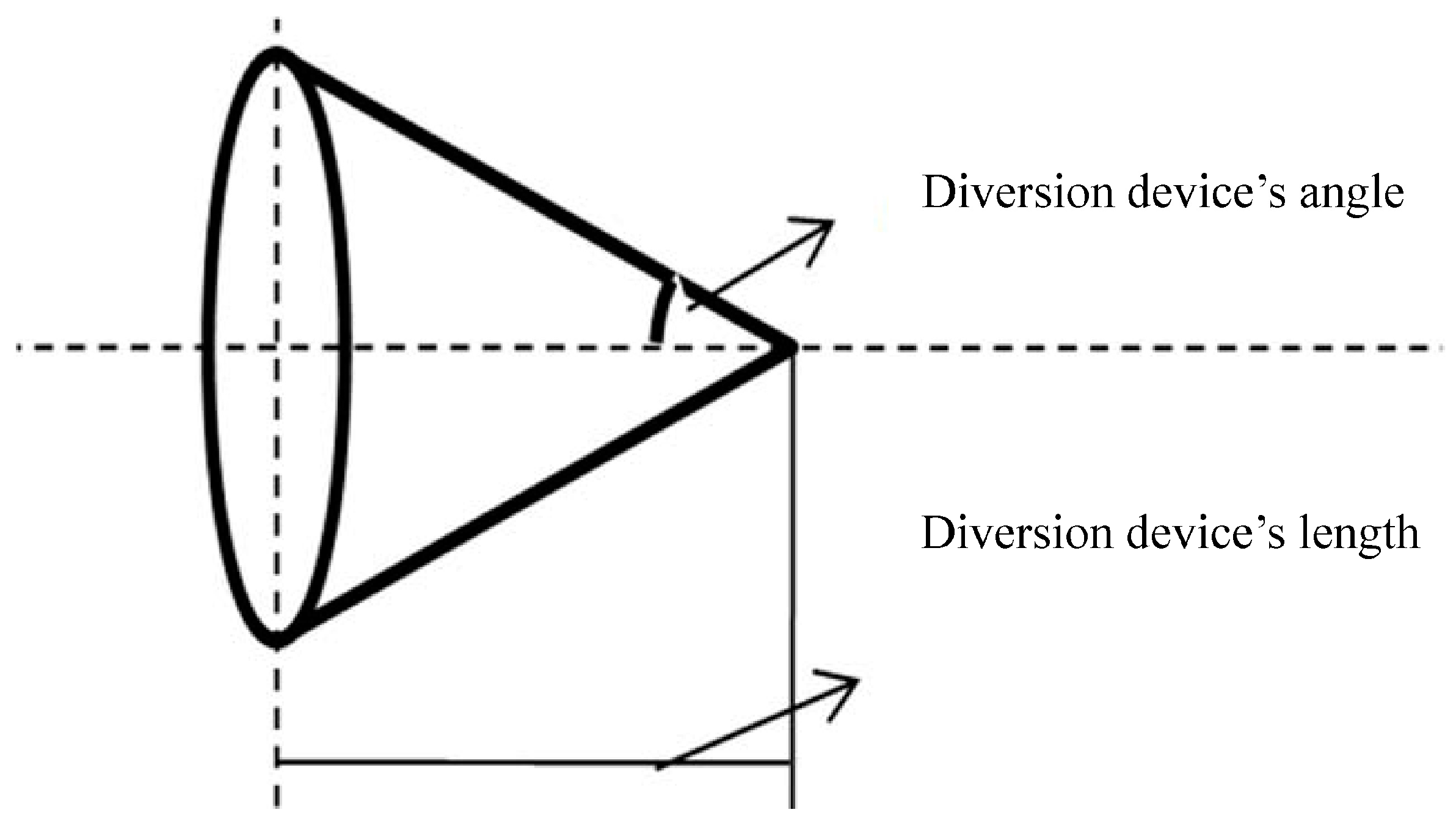
In this paper, we put a taper diversion device on the entrance of the separator; it is empty inside the diversion device and is made with highly sulfur-resistant material in order to slow down the speed of the gas; meanwhile, the diversion can be used as a drainage ability for the moist gas, and therefore, gas can be led to the separation umbrella to improve dehumidification efficiency. The structure of the diversion device is displayed in
Figure 7. With this design, the main factors which influence the ability of drainage are the angle and the length of the diversion device; we use a control variate method to simulate the perfect angle and length of the diversion device.
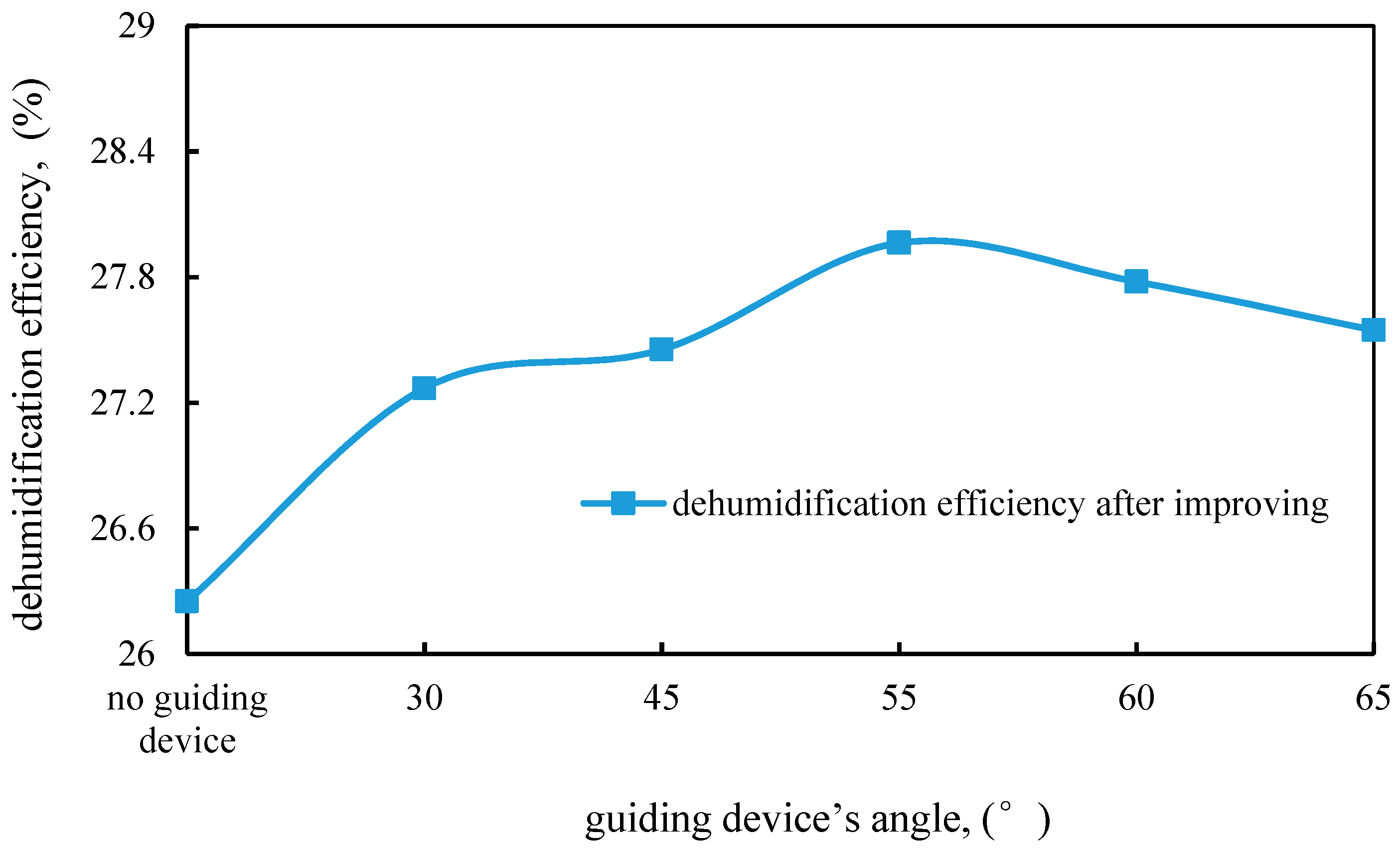
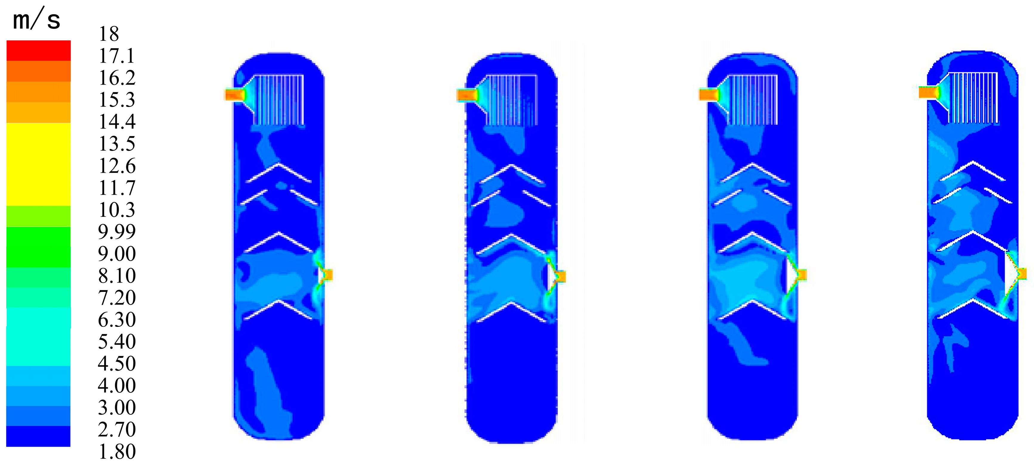
(1) Angle optimization of diversion device
Fix the horizontal length to be 200 mm, and set the percentage of the water volume to be 216 ppm and the velocity to be 15 m/s. Through the numerical simulation we can get the separation efficiency of the diversion device under different angles. The result of the simulation is displayed in
Figure 8. From left to right are the equipment without diversion device, and equipment with diversion device angles of 0°, 30°, 45°, 55°, 60° and 65°, respectively. When the angle is 30° or 45°, the diversion device has a certain extent of improvement for the cushion and changing the direction of flow, but the overall effect is obvious: Rectified gas is still eroding the surface with its large speed, and the umbrella cap is used but the effect is not obvious in the preliminary separation zone. When the angle is 55°, 60°or 65°, we can see a more improved inlet gas-flow state by the velocity field, as gas does not impact the wall, but moves to the advanced separation area again, so as to raise the separation efficiency. By studying the result of simulation, the changing rule can be seen in
Figure 9. By monitoring the export moisture content, the separation effect is shown in
Table 3.
From the result of the simulation, through comparing with the separator that is not optimized, the separation can be seen to improve a little but not too much. The best dehumidification efficiency is achieved with the angle of 55°. When the angle is larger than 55°, the upper part of the diversion device goes beyond the right part of the separation umbrella. After flowing through the diversion device, it flows across the separation umbrella and moves upside, and the dehumidification efficiency therefore reduces.
(2) Length optimization of diversion device
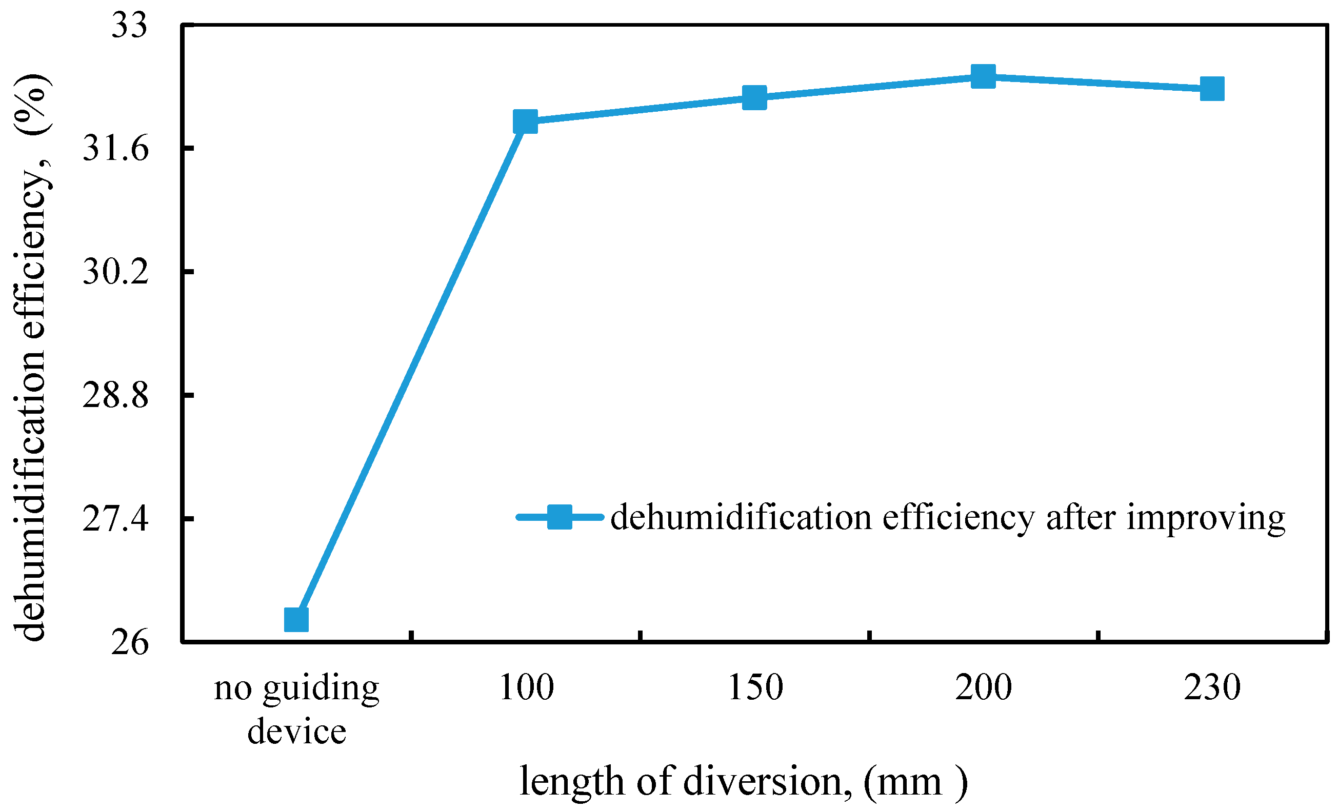
The fixed horizontal angle is 55°, while the lengths are 100 mm, 150 mm, 200 mm and 230 mm, respectively. Set the percentage of water volume to be 216 ppm, and the flow velocity to be 15 m/s. We can find the simulation results under different lengths of the diversion device by simulating the model; the results are shown in
Figure 10 and
Table 4.
As shown in
Figure 11, we can clarify the law that different lengths of diversion device influence the dehumidification efficiency. From the rule curve, we can see that when the length in the horizontal direction is 200 mm and the angle is 55°, the diversion effect is the best. Comparing with the equipment without a diversion device, the dehumidification efficiency is improved by 23.637%.
Then, this paper continues analyzing the influencing factors of the separator’s operational parameters, mainly focusing on the fluctuation of moisture content at the entrance and influence of flow rate fluctuation on separating efficiency. The result is shown in
Figure 12.
The article would improve the structure’s separating efficiency after comparing it with the original structure (no diversion device (actual situation on site) with the entrance moisture content as 2.16%, the export moisture content as 1.593%, the separation effect as 26.25%, and the prediction error as 3.41%).
From the simulation results, we can conclude that after improving the equipment, the dehumidification efficiency is improved. The separator can handle the moisture gas with high flow rate and high moisture content. The water volume percentage of the separator can basically be controlled within 300 ppm. Under the calculation conditions (216 ppm, 30 m/s), separation efficiency increases by 2.23% on average.
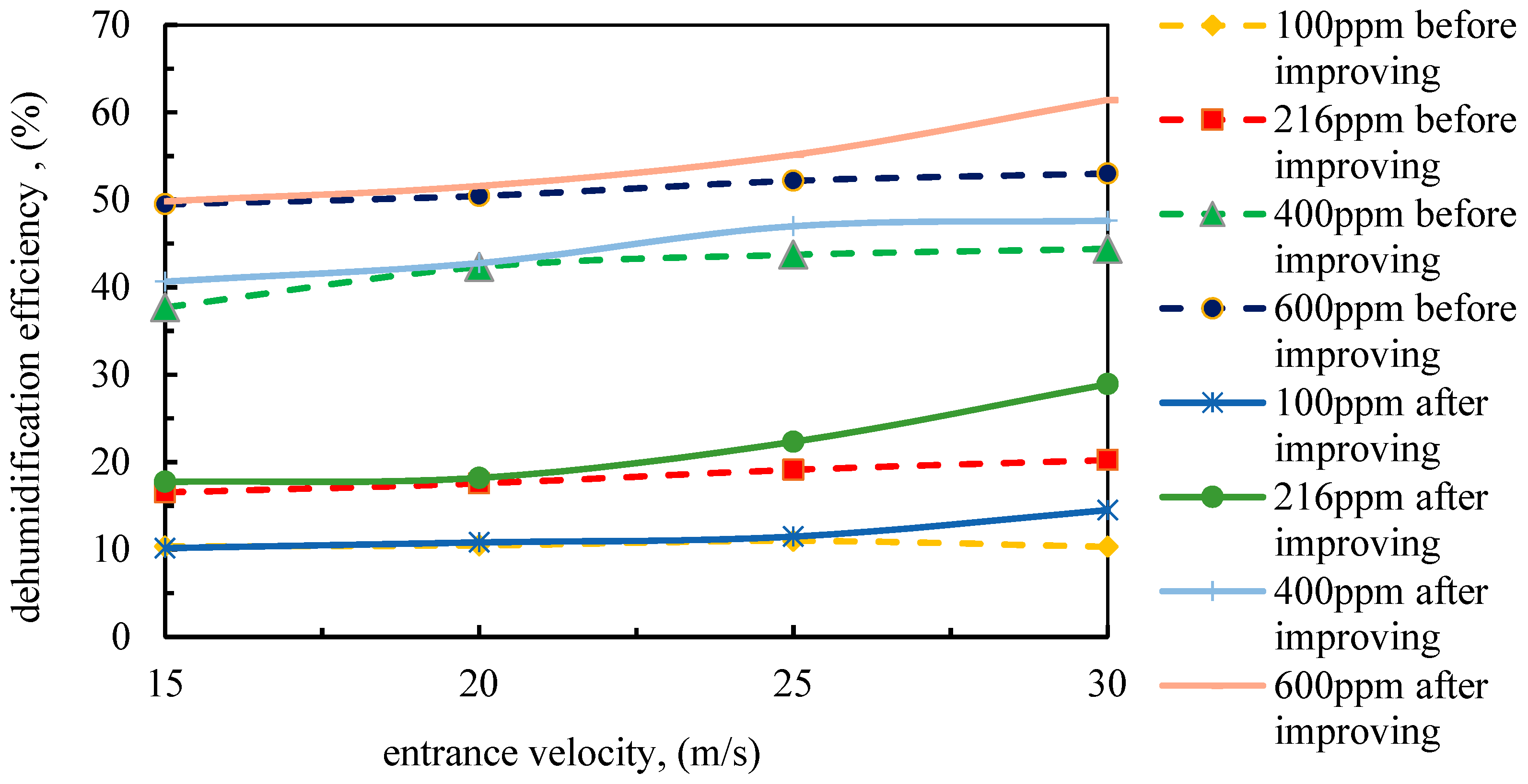
Draw the separation efficiency curve with the influence of scene condition parameter fluctuations, as shown in
Figure 13.
According to
Figure 13, we can see that the improved separator meets most of the site conditions, and under the same site conditions, separating efficiency is obviously promoted. In the face of some special scene conditions, such as unstable gas measure, the separation efficiency on the whole remains high. Therefore, this optimization design can not only solve the problem of erosion of the separator’s lining, but also increases the dehumidification efficiency.
7. Conclusions
- (1)
With the water content increased, the separating efficiency increases, meaning that the separator has the ability to handle the tail gas with high water content. The separator’s throughput should not be high, although high entrance flow rates can expand the gas’s range of motion and contribute to the collision coalescence separation efficiency, the erosion to the wall also increases, it will corrode the wall inside the separator and shorten the service life of the equipment.
- (2)
The handling capacity of the separation should be controlled to stop the gas from touching the wall inside the equipment. To solve the problem, we set up a diversion device on the entrance of the equipment contributing to movement of the gas. The gas will move in an upper direction along the middle inside the separator and increase the utilization of the preliminary separation zone as well as the fine separation zone.
- (3)
Based on the original structure of the separator (no diversion device (actual situation on site)), the moisture content of the entrance is 2.16%, the moisture content of the export is 1.593%, the separation effect is 26.25%, and the error of prediction is 3.41%. After improving the structure of the separator, processing capacity has reached 6.4–14.4 × 10⁴ m³/d, the improvement enhances the scene applicability of the separator, and we can find the fluid moisture content after entering the desulfurization tower.
- (4)
By setting up the diversion device in the entrance of the equipment (a hollow cone whose length is 200 mm at the angle of 55°), the erosion of the inside wall can be avoided. The dehumidification efficiency therefore is increased by 23.637% on average.


