Numerical Simulations of Dynamic Pipeline-Vessel Response on a Deepwater S-Laying Vessel

Abstract

The dynamic action induced on offshore pipelines by deepwater S-laying is significant, and directly determines how the pipeline structures are designed and installed. Existing research has not fully investigated the benefits of coupling models of pipeline and pipelaying vessel motions. Therefore, this paper presents a coupled time-domain numerical model for examining the effect of coupled dynamic reactions. The coupled model takes into account the motion of the pipelaying vessel, surface waves, ocean currents, wind forces, pipeline dynamics, and contact between the rollers and the pipeline. A proportional, integral, derivative (PID) controller was used for simulating the control of the pipelaying vessel. The hydrodynamic forces that the pipeline experiences were modeled using the Morison equation. The model was solved using Newmark’s method and verified using OrcaFlex software. The model was then used to analyze practical operations: the laying of a 22″ gas export pipeline on the seabed by the pipelaying vessel HYSY201 in the Pingbei-Huangyan gas fields in the East China Sea. The effects of coupled factors on pipelaying vessel motions and pipeline dynamics were approximated. These effects included configurations, axial tensions, and bending moments. The results show a significant connection between the dynamic responses of the pipelines and pipelaying vessel motions.

1. Introduction

Submarine pipelines are considered to be the most efficient and feasible means of transporting large-scale gas and oil from offshore to onshore. Deepwater pipelaying is a standardized industrial process for offshore pipeline installation and maintenance [1,2]. Installations of deepwater pipelines are implemented using the J-laying or S-laying techniques. During J-laying operations, the pipeline is lifted off the stinger in a nearly vertical position, which gives the pipeline a large bending radius from the sea surface to the seabed. Therefore, the touchdown point is relatively close to the pipelaying vessel, which makes it easy to monitor and position. The tension in the pipeline is small. However, the speed and efficiency of J-laying is lower than that of S-laying. Because all the J-laying operations are performed vertically, the vessel is not as stable as in S-laying [3]. The S-laying technique still occupies a dominant position in the current pipelaying market because of its specific advantages. S-laying has a higher adaptability and workability in different sea states and at various water depths, and it has a higher pipelaying efficiency and lower costs. In 1967, Plunkett showed that a deepwater pipeline can be assembled in an angular position on a lay barge and maintained at a predetermined high-tensile force while lowering it to the ocean bottom. This process is called S-laying. The S-laying method was developed in the 1980s and became the most frequently-used installation method [4]. In the S-laying method, the pipeline is supported using a stinger and passes over a regular roller sequence forming an S-shaped trajectory before landing on the seabed, as illustrated in Figure 1. The upper curved S-shaped parts that rest on stingers are called overbends and are followed by inflection points where the pipeline curvature is zero. Before approaching the seafloor, the pipeline is reversed into a sagbend. Horizontal tension in the pipeline is maintained by mounted tensioner devices on the top of the pipeline. Consequently, S-laying operations depend on roller configuration and stinger radius. Large plastic deformation occurs when pipes pass over stingers. The plastic deformation is caused by the combined effects of the pipelaying vessel motion, roller reaction forces, axial tensions, and bending moments [5,6].

There are several methods for analyzing pipelaying issues. These methods include static analysis, quasi-static analysis, and dynamic analysis. The natural catenary technique involves initially modeling a pipeline with asymptotic expansion, and is ideal for large, nonlinear deflections when tension has more effect on significant length than bending stiffness, and was first used in 1967 by Plunkett [7]. Dixon used the stiffened catenary technique to solve the pipeline laying problem, and computed the required pipeline inclination and tension for the pipelaying vessel [8]. Brewer examined the impact of pipelaying barge motions on suspended pipelines using quasi-static procedures and an extended stiffened catenary concept [9]. In recent years, some researchers have analyzed the S-laying pipeline configuration using the stiffened catenary technique and proposed a co-rotational finite element formulation integrated with Bernoulli’s beam theory for assessing offshore pipeline configurations and stresses in S-laying operations [10].

The abovementioned studies on modeling pipelaying issues focused on static and quasi-static analysis. Because offshore production has shifted to deepwater, it is necessary to address operation-induced dynamic pipeline laying factors using modeling. Zan et al. developed a real-time numerical model for dynamically analyzing offshore pipelaying using simulations; they included vessel motion, stratified current flow, nonuniform currents, and other dynamic factors. Their results revealed that dynamic forces were important factors that acted upon the pipeline [11]. Gong et al. created an extensive finite element model for S-laying systems that considered the contact between stinger rollers and the pipeline, pipelaying vessel motion, ocean currents, and surface waves using OrcaFlex [12]. OrcaFlex is a 3D, nonlinear, time-domain, finite element program developed by Orcina for static and dynamic analysis of marine risers and pipelaying operation systems. However, the calculations in OrcaFlex are based on the response amplitude operator (RAO) motions of the vessel. This implies that the vessel will only make slight movements at the balanced position, and be unaffected by the pipeline. Furthermore, the dynamic positioning system control model is not considered in OrcaFlex [13]. Liang et al. created a modified finite element model using the software of Abaqus to consider the complex surface contact properties within the overbend section. The contact state properties of various rollers in a single box of rollers were investigated and the emerging support torques (forces) from all roller boxes were computed and contrasted using commercial software [14]. Xie determined a pipe’s dynamic loading history for S-laying operations using a verified finite element model, and then computed residual plastic deformations for pipe cross-sections after the pipe had reached the seafloor [15]. Jensen established a model using nonlinear partial differential equations for the dynamics of pipeline strings suspended from a pipelaying vessel to the seafloor during pipelaying operations. Jensen developed his model from an existing three-dimensional beam model that described tension forces, bending moments, and shearing in sea applications; Jensen added the effects of seabed interactions, hydrodynamic drag, and restoration forces [16]. Wittbrodt employed an improved rigid finite element method to enhance computational effectiveness when a dynamic response simulation of pipelines is carried out [17].

However, none of the existing research has fully investigated, or evaluated the benefits of, coupled vessel motion and pipeline dynamics models using dynamic positioning systems. Therefore, the present paper addresses this knowledge gap by investigating a coupled vessel motion–pipeline dynamics time-domain numerical model for analyzing a pipeline’s mechanical properties in S-laying operations. The coupled numerical model incorporates, among others, pipelaying vessel motions and the contacts between stinger rollers and the pipeline. A dynamic positioning system was used to control the pipelaying vessel’s position within the coupled model. The hydrodynamic forces acting on the pipeline were considered using the Morison equation. Finally, the effects of coupled factors on the dynamic properties of offshore pipelines were extensively investigated using a practical example: the laying of a 22″ gas export pipeline on the seafloor by the pipelaying vessel HYSY201 in the Pingbei-Huangyan oil and gas fields in the East China Sea.

2. Materials and Methods

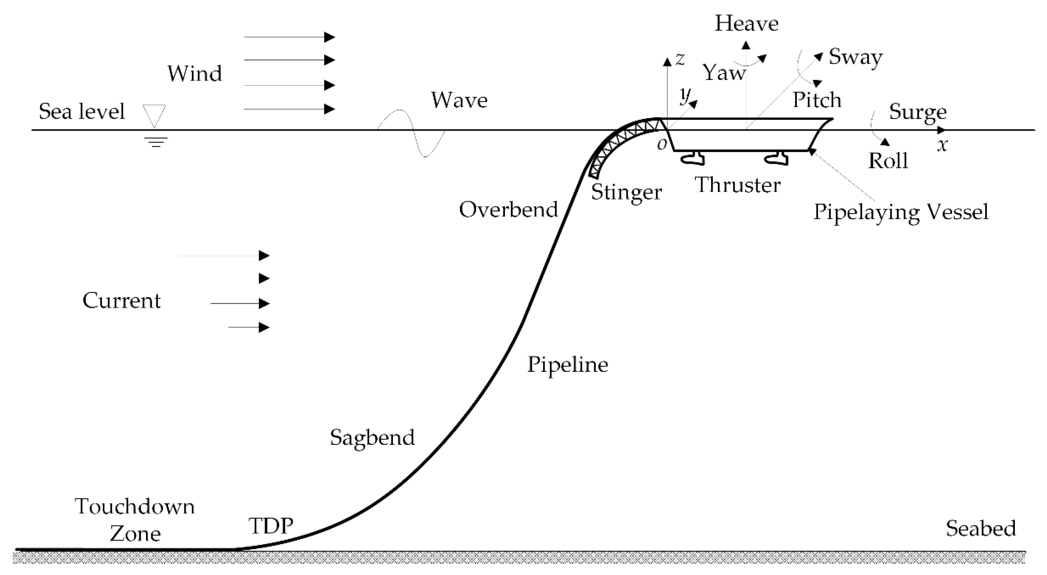
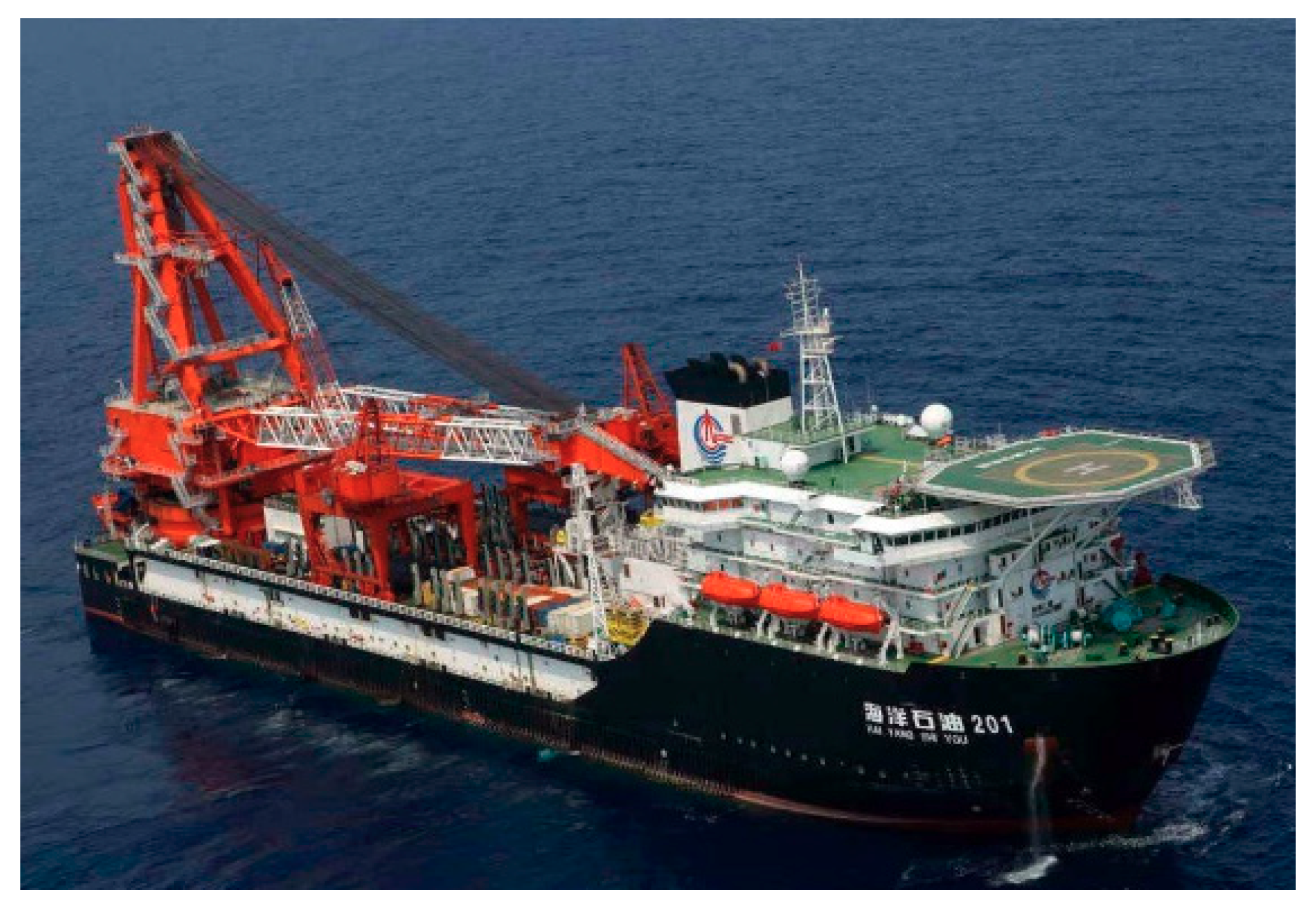
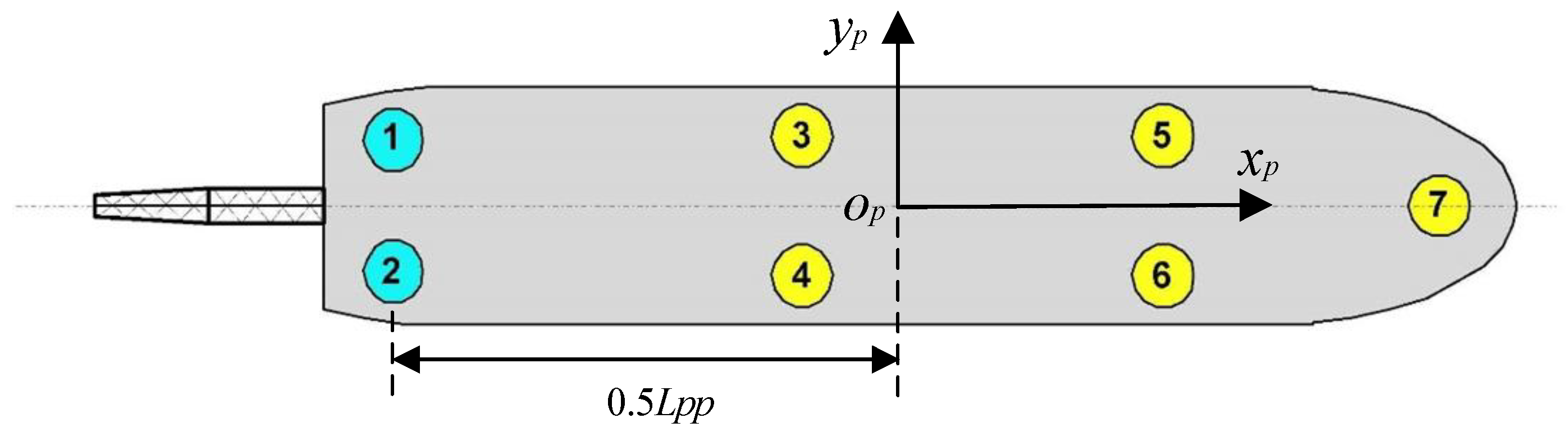
2.1. S-Laying Vessel Description

The results described are for the pipelaying vessel HYSY201—a deepwater S-laying vessel owned by China’s Offshore Oil Engineering Company Ltd. (Beijing, China) (see Figure 2). The main parameters for the pipelaying vessel with a 10% pipe load requirement are presented in

Table 1. HYSY201: pertinent specifications.

Item	Unit	Data
Overall length	m	204.65
Length between perpendiculars	m	185.00
Breadth	m	39.20
Depth	m	14.00
Mean draft	m	8
Trim	°	1
Displacement	t	47,886.7
Transverse inertia radius	m	15.93
Longitudinal inertia radius	m	55.24

. The pipelaying capacity for double-jointing systems with 6–60″ pipes and a 2 × 200-ton tensioning system, supported by a 400-ton Abandonment & Recovery capacity, is provided. The weight of the pipes that can be stored on the upper deck is 9000 tons. Pipe transferring and handling is undertaken using conveyors, rollers, and two mobile gantry deck cranes [18]. A permanent truss-type stinger and stinger adjustment system is located at the vessel aft. A dynamic positioning (DP) system has been designed that provides high redundancy and meets DP2 requirements for pipelaying operations in deepwater [19].

2.2. Equations for Coupled Motion

Using Newton’s second law, the time-domain equations of motion for the six degrees of freedom for a vessel were linearized to reach an equilibrium point:

$$\mathit{M}\ddot{\mathit{x}}(t)={\mathit{f}}_{rad}(t)+{\mathit{f}}_{hs}(t)+{\mathit{f}}_{wave}(t)+{\mathit{f}}_{exc}(t)$$

(1)

where M denotes the inertia matrix, x(t) represents the displacement vector, and t represents time. ${\mathit{f}}_{rad}(t)$ represents the radiation forces arising from the change in fluid momentum caused by the vessel’s motion, ${\mathit{f}}_{hs}(t)$ represents the hydrostatic restoration forces caused by buoyancy and gravity, and ${\mathit{f}}_{wave}(t)$ represents the wave forces acting on the vessel. In addition, ${\mathit{f}}_{exc}(t)$ represents other loads:

$${\mathit{f}}_{exc}(t)={\mathit{f}}_c(t)+{\mathit{f}}_w(t)+{\mathit{f}}_{dp}(t)+{\mathit{f}}_r(t)+{\mathit{f}}_p(t)$$

(2)

where ${\mathit{f}}_c(t)$ and ${\mathit{f}}_w(t)$ represent the current and wind forces, respectively, acting on the vessel. ${\mathit{f}}_{dp}(t)$ represents the thruster forces regulated by the DP system, ${\mathit{f}}_r(t)$ represents the reaction forces for the roller–stinger contact model, and ${\mathit{f}}_p(t)$ represents the tensional forces at the top of the pipeline that act on the vessel.

For the approximation of a linear wave, Cummins [20] used potential theory when studying hydrodynamic radiation within the time-domain of an ideal fluid and obtained the following representation.

$${\mathit{f}}_{rad}(t)=-\mathit{A}(\infty )\ddot{\mathit{x}}(t)-{\displaystyle {\int }_0^t\mathit{K}(t-\tau )}\dot{\mathit{x}}(\tau )\mathrm{d}\tau$$

(3)

where $\mathit{A}(\infty )$ represents a constant positive-definite matrix known as infinite-frequency added mass, which is linked to the displaced fluid because of the vessel’s motion. The second term represents fluid-memory, which captures the transfer of energy from the vessel’s motion into the liquid in free-surface radiated waves. The kernel of the convolution term, K(t), is the matrix of retardation or memory functions (impulse responses).

The convolution term is known as a fluid-memory model. It represents the fluid memory effects that incorporate energy dissipation caused by the radiated waves generated by the motion of the vessel. This term is not an efficient term to compute numerically because it requires information from the previous time steps, and, in theory, from the start of the body motion. Therefore, most of the existing codes using this formulation truncate the integral in Equation (4):

$${\mathit{f}}_{rad}(t)=-\mathit{A}(\infty )\ddot{\mathit{x}}(t)-{\displaystyle {\int }_{t-t_0}^t\mathit{K}(t-\tau )}\dot{\mathit{x}}(\tau )\mathrm{d}\tau$$

(4)

The accurate nature of the convolution term depends on the stored memory time quantity (t₀) and the modeling of the vessel’s impulse reaction function quality. A pipelaying vessel, which radiates few waves, does not require long-term memory values.

When a vessel’s motions are taken into account within the frequency dimension at the expense of other loads, it assumes the form [21]

$$\left\{-{\omega }^2\left[\mathit{M}+\mathit{A}(\omega )\right]+\mathrm{j}\omega \mathit{B}(\omega )+\mathit{C}\right\}\mathit{X}(\mathrm{j}\omega )={\mathit{F}}_{wave}(\mathrm{j}\omega )$$

(5)

where $\mathit{A}(\omega )$ and $\mathit{B}(\omega )$ represent the frequency-dependent added mass alongside the damping matrices. The term $\mathit{X}(\mathrm{j}\omega )$ represents the motion amplitude and phase caused by wave excitations and ${\mathit{F}}_{wave}(\mathrm{j}\omega )$ represents the linear forces caused by the waves. Ogilvie determined $\mathit{A}(\omega )$ and $\mathit{B}(\omega )$ directly by applying a Fourier transform in a sinusoidal regime [22]:

$$\mathit{A}(\omega )=\mathit{A}(\infty )-\frac{1}{\omega }{\displaystyle {\int }_0^{\infty }\mathit{K}(t)\sin (\omega t)\mathrm{d}t}$$

(6)

$$\mathit{B}(\omega )={\displaystyle {\int }_0^{\infty }\mathit{K}(t)\cos (\omega t)\mathrm{d}t}$$

(7)

Through the application of a Fourier transform, K(t) can be computed from the information for the damping matrices and added mass:

$$\mathit{K}(t)=\frac{2}{\pi }{\displaystyle {\int }_0^{\infty }\mathit{B}\left(\omega \left)\cos \right(\omega t\right)}\mathrm{d}\omega$$

(8)

$$\mathit{K}(\mathrm{j}\omega )={\displaystyle {\int }_0^{\infty }\mathit{K}\left(t\right)e^{-\mathrm{j}\omega t}}\mathrm{d}t=\mathit{B}(\omega )+\mathrm{j}\omega \left[\mathit{A}(\omega )-\mathit{A}(\infty )\right]$$

(9)

In linear theory, when the motion of the pipelaying vessel and waves are assumed to be small, the hydrostatic restoring forces are linear and proportional to the respective displacements of the body, and are simply represented by

$${\mathit{f}}_{hs}(t)=-\mathit{C}\mathit{x}(t)$$

(10)

where C is the hydrostatic restoring matrix.

2.3. Environmental Forces

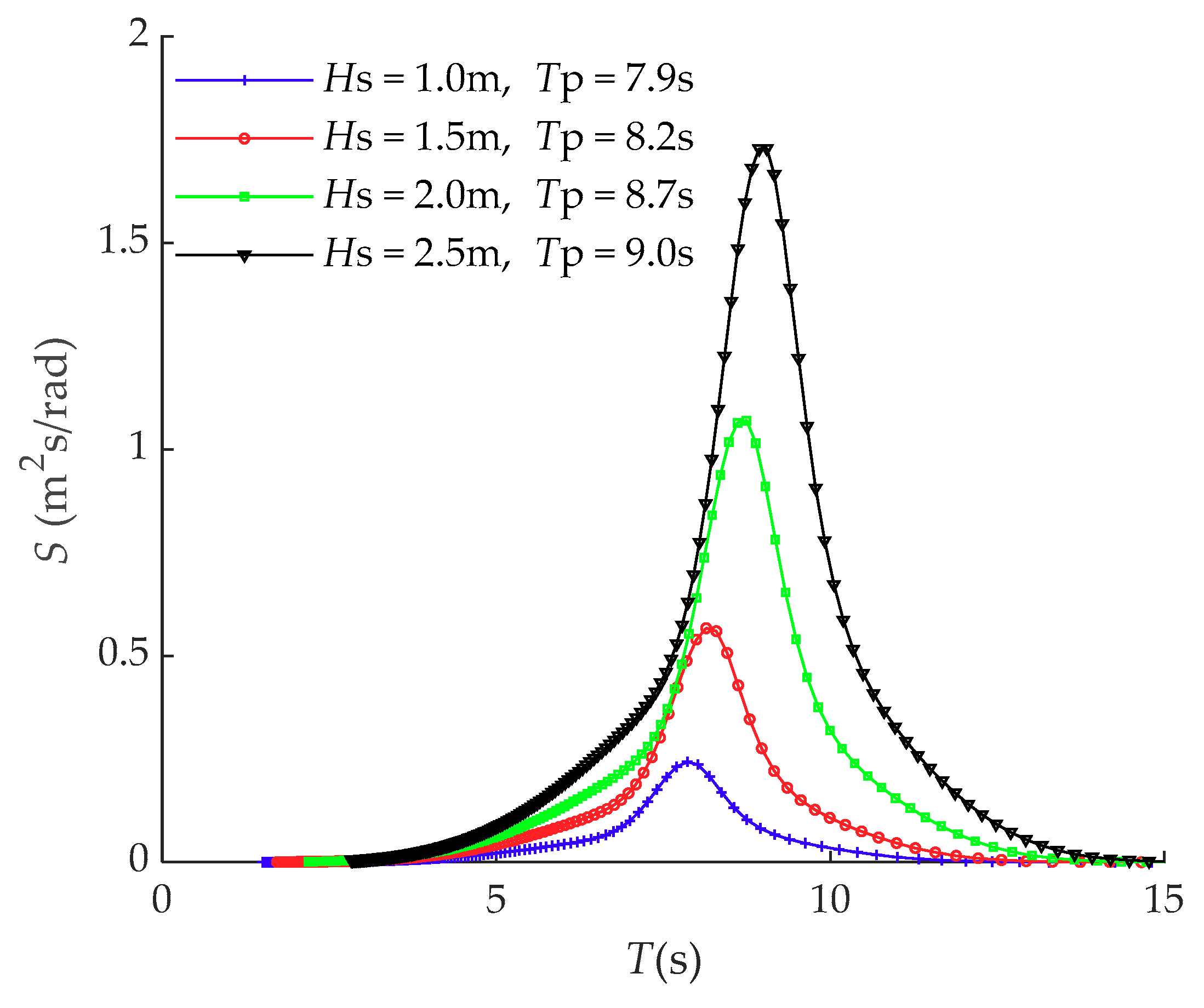
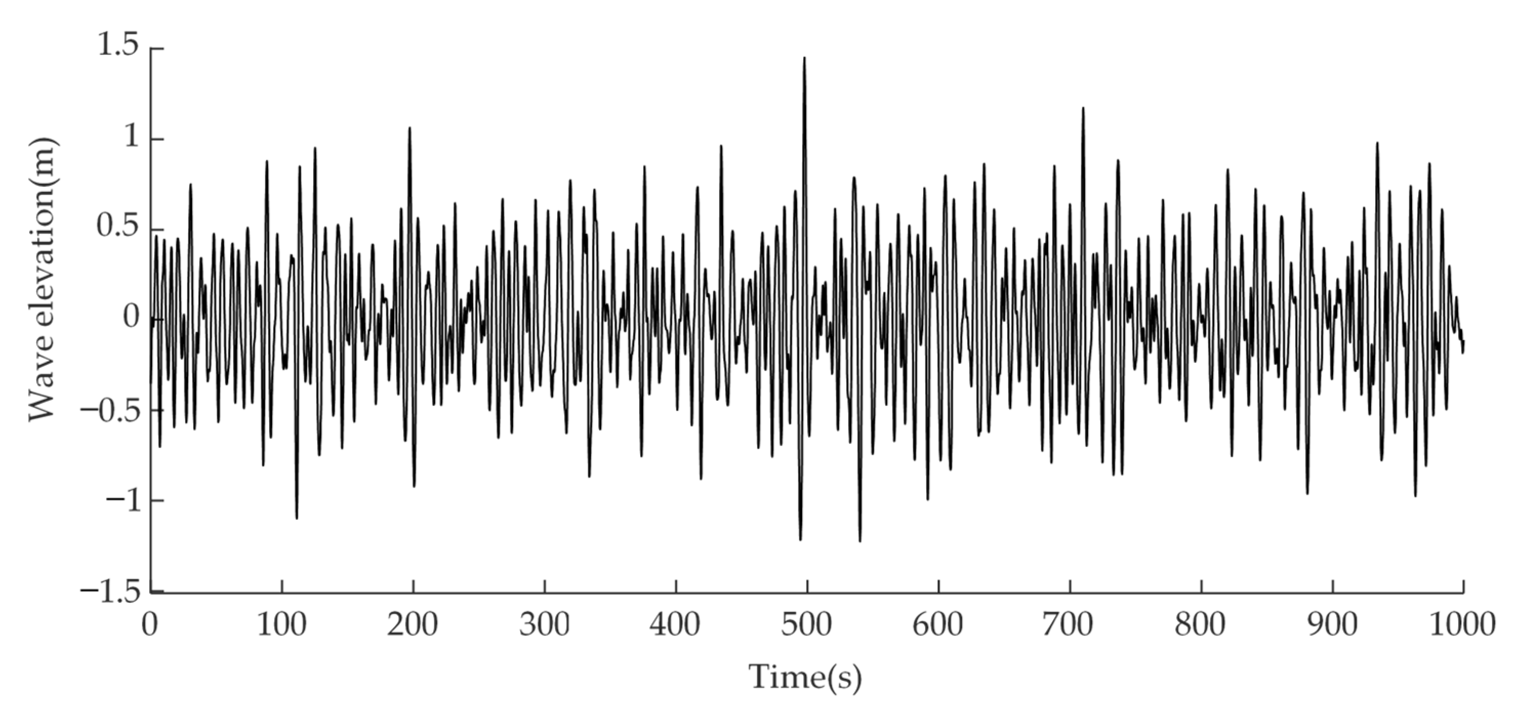
2.3.1. Wave Forces

Wave forces possess first-order wave forces and second-order slow wave drifting forces. The first-order wave forces arise from incoming waves, thus accounting for the Froude–Krylov (pressure forces caused by undisturbed wave fields) forces as well as the diffraction forces (caused by modified wave fields as a result of their structure). Average low frequency and second-order wave forces play a significant role in floating body dynamics. The horizontal parts are referred to as second-order slow wave drift forces because, under their influence, floating unrestrained vessels would drift away, and undergo a slow drifting motion along the direction of the wave. In this paper, the total first-order and second-order wave forces and moments are computed using the frequency transfer function derived through diffraction analysis and a defined wave spectral density function.

To examine the impact caused by irregular waves, the Joint North Sea Wave Project (Jonswap) spectra are used [23]. Jonswap wave spectral density refers to the function of two user-defined coefficients A and B, peak period (T_p), and significant wave heights (H_s). The density of the spectra is expressed as

$$S\left(\omega \right)=A{g}^2/{\omega }^5\exp \left[-1.25{\left({\omega }_p/\omega \right)}^4\right]B^q$$

(11)

and the exponent q is calculated by

$$q=\exp \left[-{\left(\omega -{\omega }_p\right)}^2/\left(2{\sigma }^2{\omega }_p^2\right)\right]$$

(12)

where $S\left(\omega \right)$ represents the spectral density, A is the generalized Phillips’ constant, $\omega$ is the circular frequency of the wave component, and ${\omega }_{\mathit{p}}$ is the circular wave frequency at the spectral peak.

The Phillips’ constant A can be expressed by

$$A=\frac{5}{16}{H}_s^2\frac{{\omega }_p^4}{g^2}\left[1-0.287\ln \left(B\right)\right]$$

(13)

The parameter t is presented as

$$\{\begin{array}{ll}\sigma =0.07& \omega <{\omega }_p\\ \sigma =0.09& \omega >{\omega }_p\end{array}$$

(14)

The Preakness parameter B is defined as

$$B=\{\begin{array}{ll}5& \frac{T_p}{\sqrt{H_s}}<3.6\\ \exp \left[5.75-1.15\frac{T_p}{\sqrt{H_s}}\right]& 3.6\le \frac{T_p}{\sqrt{H_s}}\le 5\\ 1& \frac{T_p}{\sqrt{H_s}}>5\end{array}$$

(15)

To determine the surface wave effects on the dynamic behavior of the pipeline in deepwater S-laying operations, the corresponding Jonswap spectra for all specific wave conditions, four sea states containing varying significant wave heights, and peak periods were considered (Figure 3).

The superposition principle is employed for building irregular sea states. The law of superposition states that problems can be broken down into different subproblems, with each subproblem carrying its solution. The solution for the entire issue is then considered as the total of the subproblem solutions. Therefore, when several wave components with a frequency ${\omega }_i$ and wave amplitude ${\zeta }_{ai}$ undergo superposition, the outcome is irregular waves. The waves’ overall motion featuring n wave components can be explained by the velocity potential below.

$$\Phi \left(x,y,z,t\right)={\displaystyle \sum _{i=1}^n\frac{{\zeta }_{ai}g}{{\omega }_i}}\frac{\cosh k_i(z+h)}{\cosh k_{i}h}\cos ({\omega }_{i}t-k_{i}x\cos {\beta }_i-k_{i}y\sin {\beta }_i+{\epsilon }_i)$$

(16)

where h represents the depth of water, $k_i$ represents the wave number, ${\beta }_i$ represents the main wave propagation direction, and ${\epsilon }_i$ represents the wave’s phase angle.

The amplitude of the wave can be obtained from the spectra $S({\omega }_i)$ and spreading function $D({\beta }_i)$ of the wave:

$${\zeta }_{ai}=\sqrt{2S({\omega }_i)D({\beta }_i)\mathrm{d}\omega \mathrm{d}\beta }$$

(17)

The first-order wave forces are computed within the time domain as

$${\mathit{f}}_{wave1}(t)=\frac{1}{4{\mathsf{\pi }}^2}{\displaystyle {\int }_{-\infty }^{\infty }{\displaystyle {\int }_{-\infty }^{\infty }{\mathit{H}}^{(1)}(\omega )}}{e}^{-i\omega \tau }\mathrm{d}\omega \zeta (t-\tau )\mathrm{d}\tau$$

(18)

where ${\mathit{H}}^{(1)}(\omega )$ represents the first-order transfer function between wave elevation and excitation force, and was computed using WAMIT [24] software. WAMIT was developed by Lee and Newman, and uses the 3D numerical panel method to solve the linearized hydrodynamic radiation and diffraction problems for the interaction of surface waves with a vessel.

The quadratic transfer function (QTF) is used for computing linear wave drift forces:

$${\mathit{f}}_{wave2}(t)={\displaystyle {\int }_0^{\infty }2{\mathit{H}}^{(2)}(\omega )S(\omega )\mathrm{d}\omega }$$

(19)

where ${\mathit{H}}^{(2)}(\omega )$ is the desired QTF, and is also computed using WAMIT software.

Thus, the resulting wave forces are

$${\mathit{f}}_{wave}(t)={\mathit{f}}_{wave1}(t)+{\mathit{f}}_{wave2}(t)$$

(20)

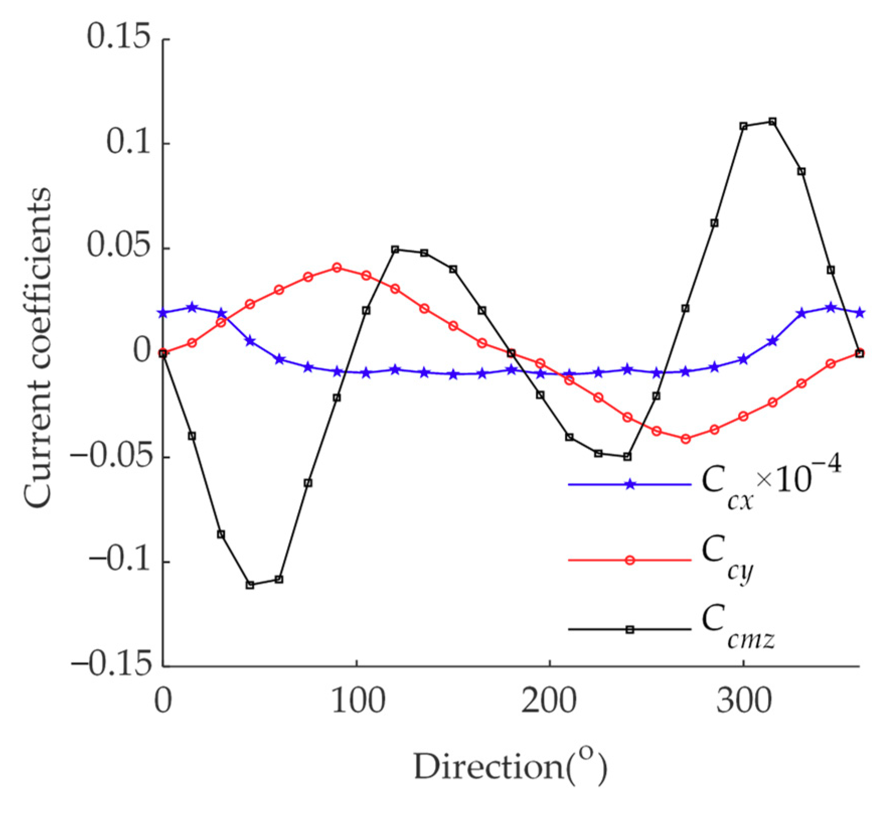
2.3.2. Current Forces

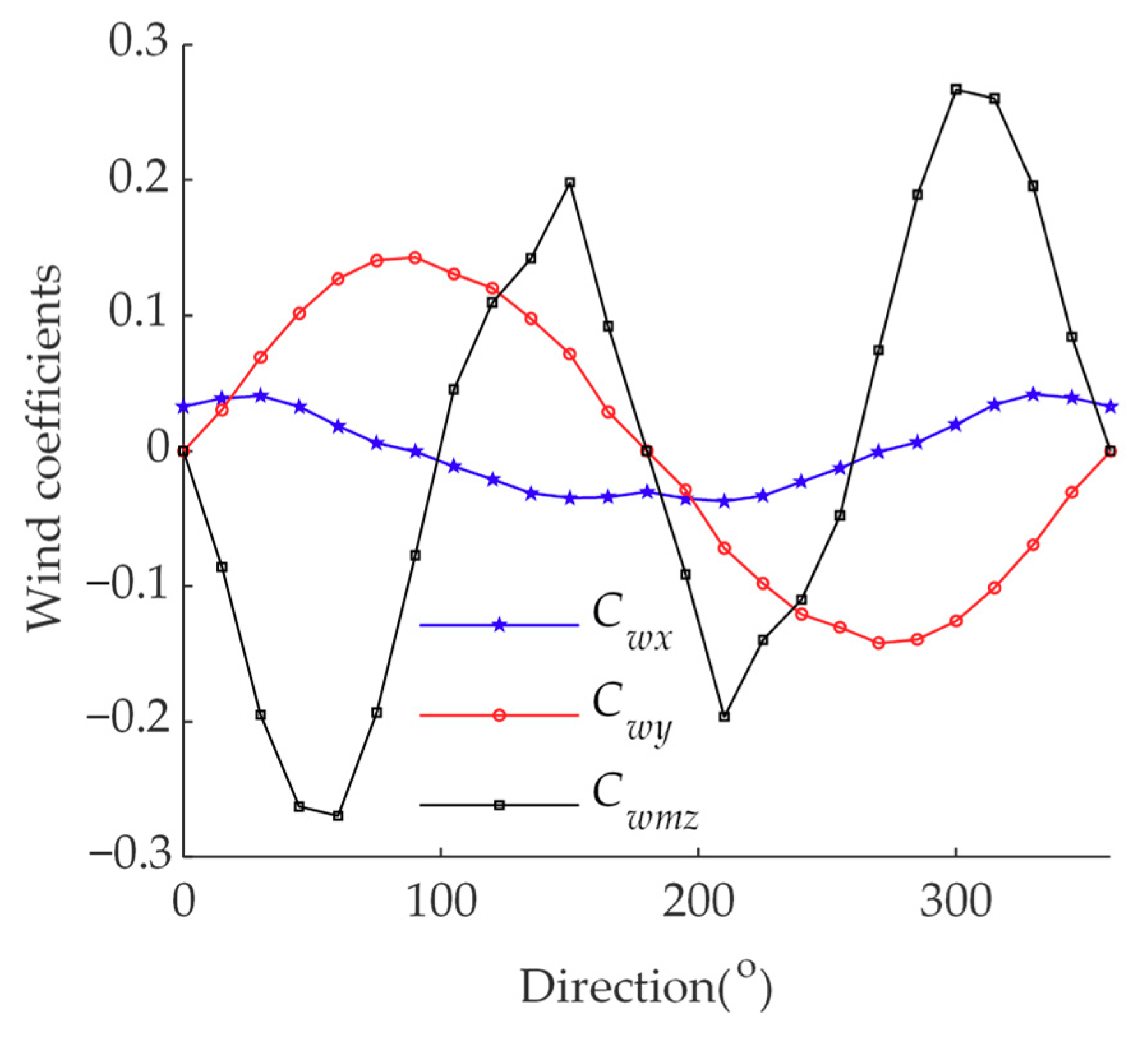
The current forces acting upon the vessel were computed during every time step, based on definitions provided by OCIMF (Oil Companies International Marine Forum) [25]. The formulae below for the surge, sway, and yaw directions were employed.

$$\{\begin{array}{l}{F}_{cx}(t)=0.5{\rho }_w{C}_{cx}{V}_c^2{L}^2\\ F_{cy}(t)=0.5{\rho }_w{C}_{cy}{V}_c^2{L}^2\\ M_{cmz}(t)=0.5{\rho }_w{C}_{cmz}{V}_c^2{L}^{2}T\end{array}$$

(21)

where ${\rho }_w$ represents the density of water; L represents the vessel’s overall length; T represents the draught of the vessel; V_c is the relative velocity between the vessel and the surface current of the sea; and $C_{cx}$, $C_{cy}$, and $C_{cmz}$ represent nondimensional current coefficients in a longitudinal direction, lateral direction, and yaw moment direction, and can be obtained through basin modeling or wind tunnel tests. In this study, the current coefficients for HYSY201 are based on data derived from wind tunnel tests (Figure 4).

The current forces in the surge, sway, and yaw directions can be calculated. The DP system is designed only to control the vessel motion on the horizontal plane, which includes the surge, sway, and yaw. During pipelaying operations, the vessel motion in the other three directions has little influence on the operations. Thus, the forces in the other three directions can be ignored, and the current forces can be expressed as

$${\mathit{f}}_c(t)={\left[\begin{array}{cccccc}{F}_{cx}(t)& F_{cy}(t)& 0& 0& 0& M_{cmz}(t)\end{array}\right]}^T$$

(22)

2.3.3. Wind Forces

Wind forces acting on bodies were also computed for every time step. A varying or constant wind direction and velocity can be simulated. Different kinds of spectra exist within the model. Alternatively, user-defined time traces can be used. The OCIMF [25] formulae below were employed for the calculation of wind forces in the directions of surge, sway, and yaw.

$$\{\begin{array}{l}{F}_{wx}(t)=0.5{\rho }_a{C}_{wx}{V}_w^2{L}^2\\ F_{wy}(t)=0.5{\rho }_a{C}_{wy}{V}_w^2{L}^2\\ M_{wmz}(t)=0.5{\rho }_a{C}_{wmz}{V}_w^2{L}^{2}T\end{array}$$

(23)

where $V_w^{}$ represents the relative velocity between the vessel and the wind, and $C_{wx}$, $C_{wy}$, and $C_{wmz}$ are the desired nondimensional wind coefficients in the longitudinal, lateral, and yaw moment directions. Wind tunnel tests are the most accurate means of estimating wind forces on offshore structures and vessels. The coefficients for HYSY201 are based on data derived from wind tunnel tests, as illustrated in Figure 5.

As in the calculation for current forces, the wind forces in the heave, roll, and pitch directions are ignored. Thus, the wind forces can be expressed as

$${\mathit{f}}_w(t)={\left[\begin{array}{cccccc}{F}_{wx}(t)& F_{wy}(t)& 0& 0& 0& M_{wmz}(t)\end{array}\right]}^T$$

(24)

2.4. Dynamic Positioning System Control Model

Dynamic positioning (DP) is a computer-guided system for automatically maintaining the position and direction of a vessel using the vessel’s thrusters and propellers. Position reference sensors coupled with gyro compasses, motion sensors, and wind sensors supply information regarding the direction of environmental forces influencing the vessel’s position, magnitude, and position. This paper presents a simulation of the DP time domain to dynamically determine whether pipelaying vessels can maintain their positions. The simulation for the time domain was realized for DP vessel motion using a mathematical model [26].

A PID (proportional–integral–derivative) controller was used for simulating the pipelaying vessel’s position. It has been extensively used in engineering and is a stable and simple control system. The controller corrects velocity and position errors, which are then eliminated by the thrusters. The PID’s nonlinear horizontal-plane positioning feedback controller is given by [27]

$$\begin{gathered} {\mathit{f}}_{dp}=K_D\dot{\epsilon }(t)+K_P\epsilon (t)+K_I{\displaystyle {\int }_0^t\epsilon (\tau )}\mathrm{d}\tau +{\mathit{f}}_w \\ \epsilon (t)=x_0(t)-x(t) \\ \dot{\epsilon }(t)={\dot{x}}_0(t)-\dot{x}(t) \end{gathered}$$

(25)

where ${\mathit{f}}_{dp}$ represents the desired control force from the thrusters, $\epsilon \left(t\right)$ represents the position error, K_P represents the position feedback gains, K_I is the desired integral feedback gain, K_D represents the velocity feedback gains, ${\mathit{f}}_w$ represents the wind feedforward forces, x(t) is the desired filtered position, and x₀(t) is the target position. The arrangement and position of the HYSY201 thrusters are illustrated in Figure 6 and summarized in

Table 2. The position of the thrusters for HYSY201.

No.	Type	x Direction Position/m	y Direction Position/m	Rotating Speed/rpm	Thruster Diameter	Maximum Thrust/kN
1	azimuth	−92.50	9.45	181	3.6	680
2	Azimuth	−92.50	−9.45	181	3.6	680
3	azimuth	−11.25	15.40	192	3.2	540
4	azimuth	−11.25	−15.40	192	3.2	540
5	azimuth	39.15	14.00	192	3.2	540
6	azimuth	39.15	−14.00	192	3.2	540
7	azimuth	54.21	0	192	3.2	540

.

The vessel’s positioning model was separated into low frequency (LF) components and high frequency (HF) components. Thrusters control the LF motions. The DP system is sensitive to high-frequency noise in the velocity and position signals because the noise undergoes amplification and is transported to the thrusters. To address this, the positions and velocities were modified using a Kalman filter. First, motion constructs were inserted using position reference systems and compared with the required position. Previously computed position predictions were then modified using a Kalman gain matrix. The Kalman gain matrix is related to cutoff frequencies, which were selected on the basis of natural durations of motions and on-wave frequency motions [28].

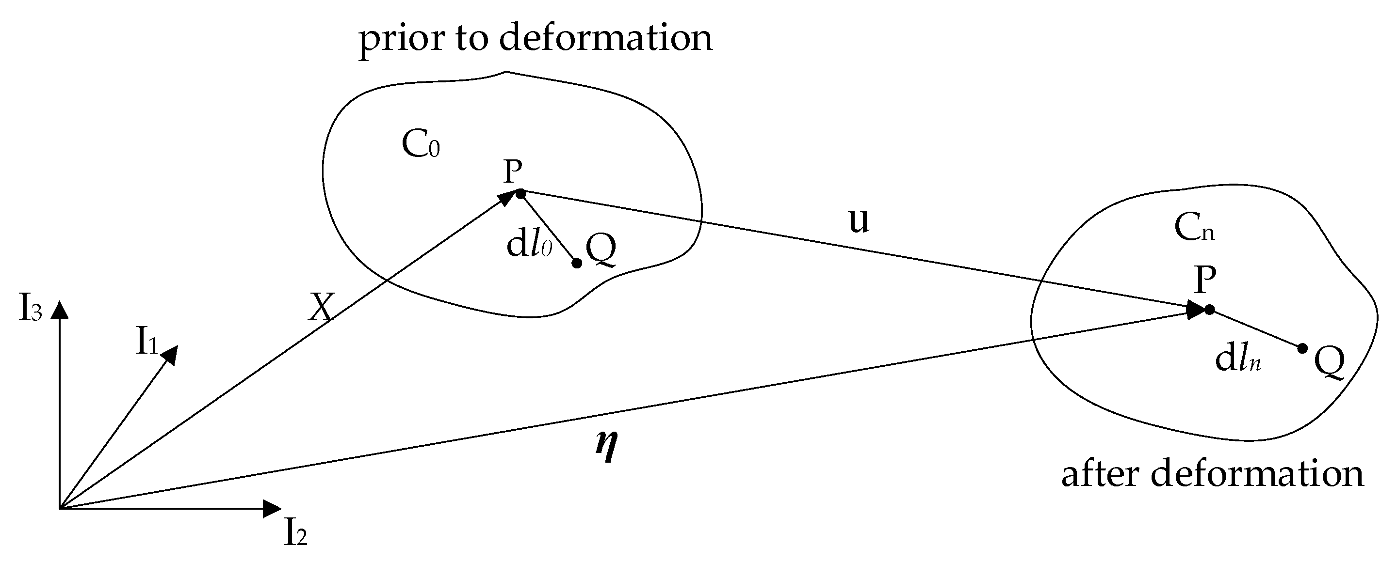
2.5. Pipeline Dynamics: Model Theory

2.5.1. Pipeline Model

The model uses the finite element method and is based on continuum mechanics principles. Lagrangian descriptions were used to describe the pipeline motions. As shown in Figure 7, the particle motion can be represented as

$$\mathbf{\eta }=\mathbf{\eta }\left(\mathit{X},t\right)$$

(26)

where X indicates the particle’s position vector and $\mathbf{\eta }$ represents the particle’s position at time t. Definition of the displacement vector u is achieved through

$$\mathbf{\eta }=\mathit{X}+\mathit{u}$$

(27)

For the Lagrangian formulation, measurement of strains is undertaken using the Green strain tensor E. The strain tensor is expressed as

$$\mathrm{d}{l}_n{}^2-\mathrm{d}{l}_0{}^2=2\mathrm{d}\mathit{X}\cdot \mathit{E}\cdot \mathrm{d}\mathit{X}$$

(28)

where $\mathrm{d}{l}_0$ and $d{l}_n$ represent the line segment PQ’s length after, and prior to, deformation, respectively. Additionally, an ideal stress measure is required during the analysis. In most instances, the symmetric Piola–Kirchhoff stress tensor l is used with the Green strain.

Malvern [29] is referred to for the detailed theory of the pipeline model. The virtual work equation can be used for expressing a finite body’s equilibrium. Using Green strains and Piola–Kirchhoff stresses, the equation can be expressed as

$${\displaystyle {\int }_{V_0}\mathit{l}:\delta \mathit{E}\mathrm{d}{V}_0}={\displaystyle {\int }_{A_0}{\mathit{t}}_0}\cdot \delta \mathit{u}\mathrm{d}{A}_0+{\displaystyle {\int }_{V_0}{\mathit{f}}_0\cdot \delta \mathit{u}\mathrm{d}{V}_0}$$

(29)

where the colon (:) notation indicates an inner product, $\delta$ represents virtual quantities, and $V_0$ and $A_0$ represent the volume and surface of the first reference configuration, respectively. Body forces ${\mathit{f}}_0$ and surface traction ${\mathit{t}}_0$ represent the unit volume and unit surface within the initial state of reference. Consequently, the equation for the dynamic equilibrium in terms of virtual work can be expressed as

$${\displaystyle {\int }_{V_0}\mathit{l}:\mathit{E}\mathrm{d}{V}_0}+{\displaystyle {\int }_{V_0}{\rho }_0\ddot{\mathit{u}}\delta \mathit{u}\mathrm{d}{V}_0}+{\displaystyle {\int }_{V_0}\tilde{c}\dot{\mathit{u}}\delta \mathit{u}\mathrm{d}{V}_0}={\displaystyle {\int }_{A_0}{\mathit{t}}_0}\cdot \delta \mathit{u}\mathrm{d}{A}_0+{\displaystyle {\int }_{V_0}{\mathit{f}}_0\cdot \delta \mathit{u}\mathrm{d}{V}_0}$$

(30)

where ${\rho }_0$ represents mass density and $\tilde{c}$ indicates a function of viscous damping density. Damping forces are proportional to velocity. The forces of inertia are proportional to the structure’s acceleration and mass. The finite element nodal points may have up to six degrees of freedom (three translations and three rotations). Finite rigid bodies can be introduced at the nodes. Thus, the tensional forces at the top of the pipeline ${\mathit{f}}_p(t)$ can be obtained [30].

2.5.2. Hydrodynamic Forces Acting on the Pipeline

Hydrodynamic in-line forces from currents acting on the pipeline apply to an accelerated fluid setting in which the pipeline is kept vertical and stationary:

$${\mathit{f}}_h=0.5{\rho }_w{C}_{d}D\mathit{u}\left|\mathit{u}\right|+{\rho }_w{C}_{m}A\dot{\mathit{u}}+{\rho }_{w}A\dot{\mathit{u}}$$

(31)

Equation (31) is known as the Morison equation [31]. In this equation, ${\rho }_w$ represents the density of water, D is the outer diameter of the pipeline, A represents the cross-sectional area of the pipeline, u represents the velocity of the fluid, C_d represents the drag coefficient, and C_m represents the hydrodynamic mass. The drag and mass coefficients depend on several parameters, including the ratio of surface roughness, a relative current value, the Keulegan–Carpenter number, and the Reynolds number. The drag and mass coefficients should be determined empirically [32].

When the pipeline is in motion and oceans currents are present during pipelaying operations, Equation (31) can be simplified for hydrodynamic force per unit length as

$${\mathit{f}}_h=-0.5{\rho }_w{C}_{d}D{\mathit{v}}_{\mathit{r}}\left|{\mathit{v}}_{\mathit{r}}\right|-{\rho }_w{C}_{m}A{\dot{\mathit{v}}}_{\mathit{r}}+{\rho }_{w}A{\dot{\mathit{v}}}_{\mathit{c}}$$

(32)

where v_r =v −v_c represents relative velocity, v_c represents the velocity of the ocean current, and v represents the pipeline’s velocity. It should be noted that the Froude–Krylov force is independent of v because the force is linked to the fluid’s absolute motion. It is assumed that ocean currents vary gradually; this implies that ${\dot{\mathit{v}}}_{\mathit{c}}\approx 0$ and the Froude–Krylov term can be discarded.

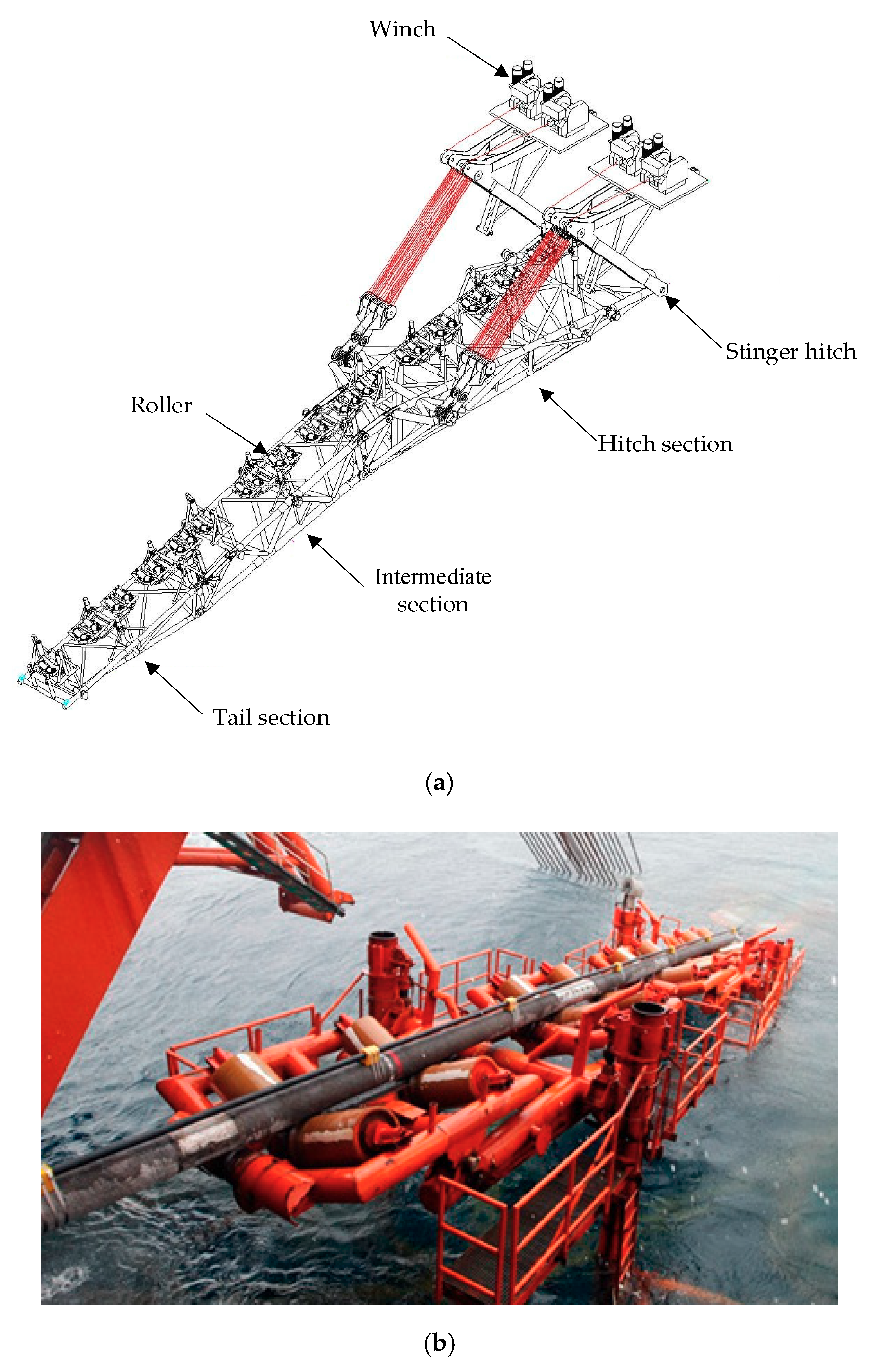
2.6. Roller: Simplifying Assumptions

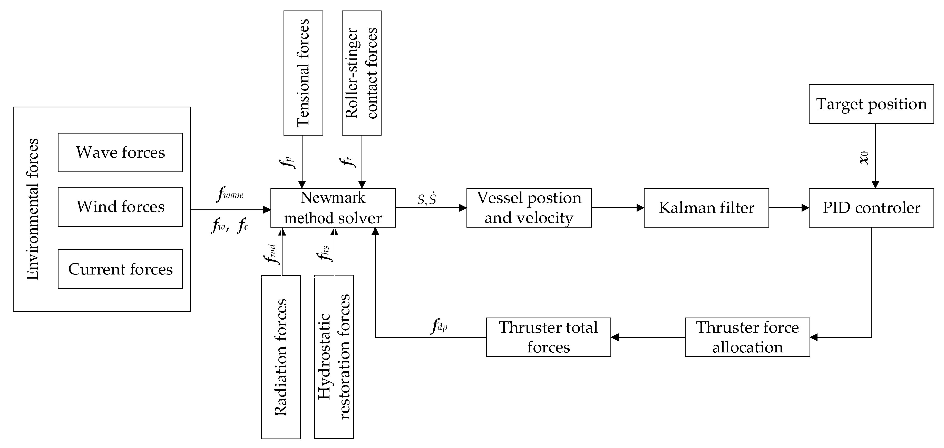
On pipelaying vessels, the pipeline is usually supplied by multiple discrete rollers. For example, the stinger of HYSY201 has three sections: a tail section, an intermediate section, and a hitch section, with lengths of 19.6 m, 22.9 m, and 33.2 m, respectively. Ten boxes of regularly spaced rollers are on the stingers, as illustrated in Figure 8a; it can be seen that the pipeline is in contact with the stinger rollers as shown in Figure 8b.

In practice, the vertical heights of all roller boxes could be modified slightly to meet the pipelaying conditions prior to offshore pipeline installation. The roller boxes support the pipeline on the stinger, and pipelaying barges prevent the pipelines’ downward lateral and vertical displacement. All rollers within the roller boxes are analyzed to ascertain if the pipelines are in contact with the rollers, and then support requirements are computed and applied to the rollers and pipes. In this paper, it is assumed that the rollers are cylindrical, and that the support acts in directions that are mutually perpendicular towards the pipelines’ longitudinal axes and all supporting rollers. The contact forces of the roller acting on the pipeline can be calculated by linear stiffness k_s [33]:

$${\mathit{f}}_r\left(t\right)=k_s\left(0.5D-\mathbf{\delta }\right)$$

(33)

where D represents the pipe diameter and $\mathbf{\delta }$ represents the distance between two straight lines on different surfaces.

3. Model Solution

Newmark’s integral method was used to solve Equation (1), in which the velocity and displacement of the vessel–pipeline system during the instant $t+\Delta t(i+1)$ can be expressed as

$$\{\begin{array}{l}{\mathit{S}}_{i+1}={\mathit{S}}_i+{\dot{\mathit{S}}}_i\Delta t+\left[\left(\frac{1}{2}-\beta \right){\ddot{\mathit{S}}}_i+\beta {\ddot{\mathit{S}}}_{i+1}\right]\Delta t^2\\ {\dot{\mathit{S}}}_{i+1}={\dot{\mathit{S}}}_i+\left(1-\delta \right){\ddot{\mathit{S}}}_i\Delta t+\delta {\ddot{\mathit{S}}}_{i+1}\Delta t\end{array}$$

(34)

where $\mathit{S}$ is the matrix of the pipelaying vessel displacement for the six degree freedom in surge, sway, heave, roll, pitch, and yaw directions; $\Delta t$ represents the time step length; and β and δ represent parameters associated with stability and accuracy, respectively.

Using Equation (34), the acceleration and velocity at the instant i + 1 is approximated using the displacements at the instant i + 1 and the instant i:

$$\{\begin{array}{l}{\dot{\mathit{S}}}_{i+1}=\frac{\delta }{\beta \Delta t}\left({\mathit{S}}_{i+1}-{\mathit{S}}_i\right)+\left(1-\frac{\mathsf{\delta }}{\beta }\right){\dot{\mathit{S}}}_i+\left(1-\frac{\mathsf{\delta }}{2\beta }\right){\ddot{\mathit{S}}}_i\Delta t\\ {\ddot{\mathit{S}}}_{i+1}=\frac{\delta }{\beta \Delta t^2}\left({\mathit{S}}_{i+1}-{\mathit{S}}_i\right)-\frac{1}{\beta \Delta t}{\dot{\mathit{S}}}_i+\left(1-\frac{1}{2\beta }\right){\ddot{\mathit{S}}}_i\end{array}$$

(35)

Substitution of Equation (35) into Equation (1) and simplification produces the equation

$$\mathit{M}\frac{1}{\beta \Delta t^2}{\mathit{S}}_{i+1}={\mathit{f}}_{i+1}+\mathit{M}\left[\frac{1}{\beta \Delta t^2}{\mathit{S}}_i+\frac{1}{\beta \Delta t}{\dot{\mathit{S}}}_i-\left(1-\frac{1}{2\beta }\right){\ddot{\mathit{S}}}_i\right]$$

(36)

${\mathit{f}}_{i+1}$ represents all the forces input into the system, including environmental forces (${\mathit{f}}_{wave}$, ${\mathit{f}}_w$, and ${\mathit{f}}_c$), radius forces (${\mathit{f}}_{rad}$), hydrostatic forces (${\mathit{f}}_{hs}$), tensional forces (${\mathit{f}}_p$) at the top of the pipeline that act on the vessel, and roller–stinger contact forces (${\mathit{f}}_r$). The responses of the system, including accelerations, velocities, and displacements at the instant i + 1 were derived by substituting Equation (36) into Equation (35) and simplifying. Then, these results were input into the DP system to be compared with the target position to obtain the deviation. Based on the deviation, the thrusters produce specific forces and feed them back to the Newmark method solver to run the calculation in the next step. Thus, the vessel will be maneuvered, step by step, to the target position. The solution procedure for the coupled model is shown in Figure 9.

4. Results and Discussion

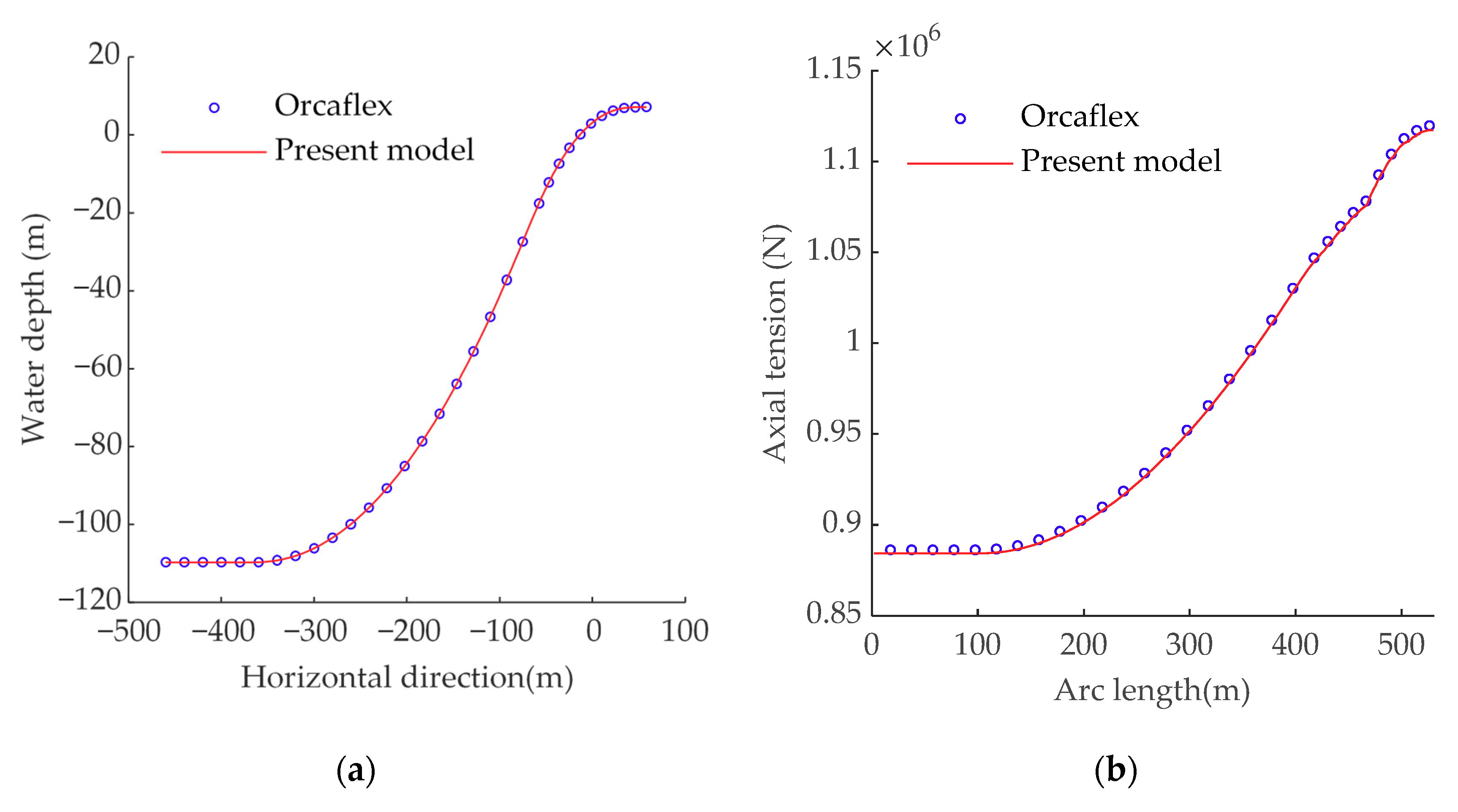
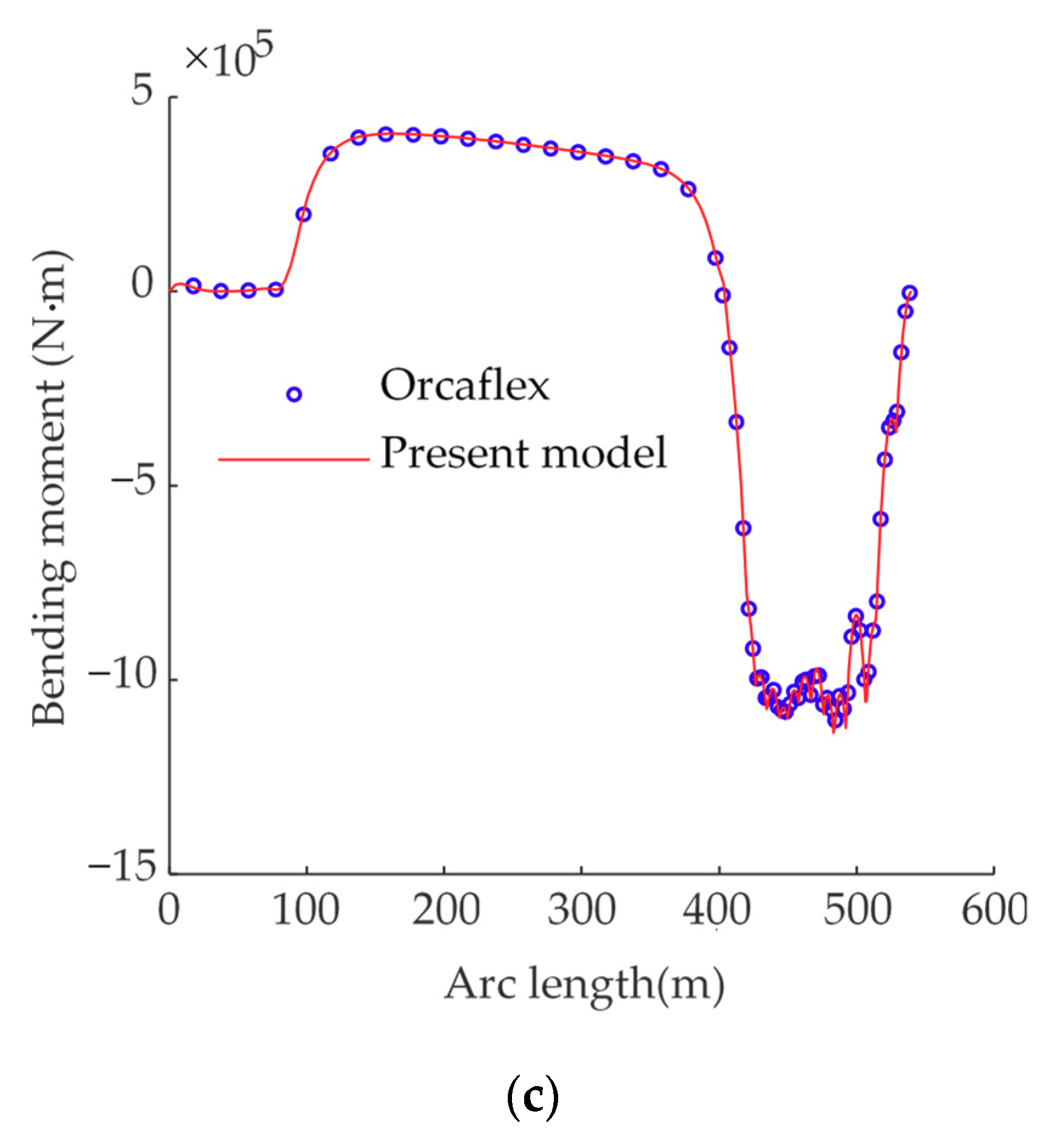
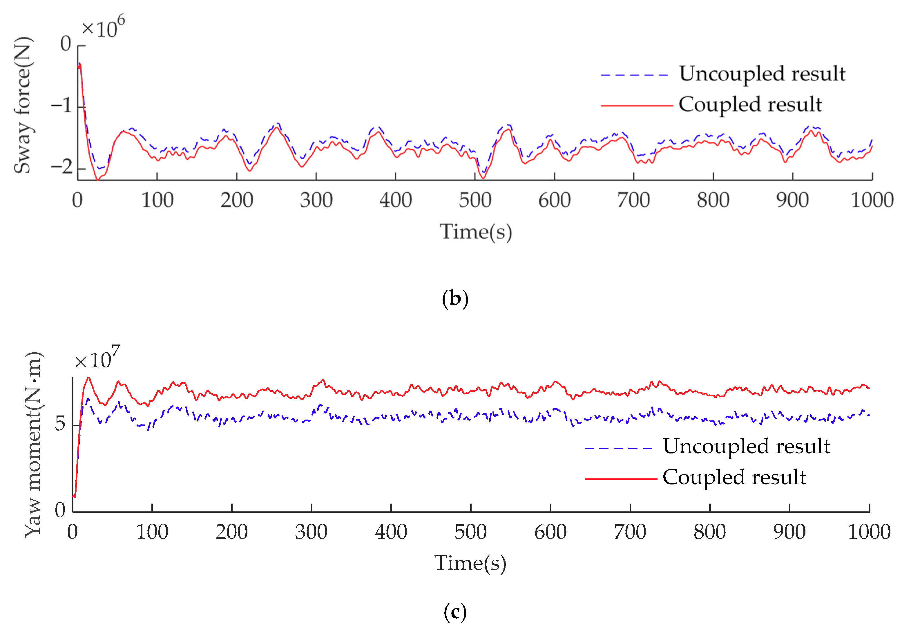
4.1. Verification and Comparison

The model data originate from a practical engineering program for the Pingbei-Huangyan oil and gas fields, located in the East China Sea, the People’s Republic of China. The oil and gas fields are approximately 425 km southeast of Shanghai. The pipeline parameters for the 22″ gas pipeline are shown in

Table 3. Parameters for the 22″ gas pipeline.

Description	Unit	Value
Outer diameter	m	0.599
Wall thickness	m	0.0159
Steel density	kg/m3	7.8 × 103
Poisson ratio	/	0.3
Elastic modulus	N/m2	2.07 × 1011
Concrete coating thickness	m	0.06
Concrete coating density	kg/m3	2.95 × 103
Anticorrosion coating thickness	m	0.0035
Anticorrosion coating density	kg/m3	940
Joint length	m	12.2

. A fixed stinger was placed at the stern of the HYSY201 for launching the pipe into the water with a suitable curvature (radius of 200 m). A water depth of 110 m and a soft seabed with a normal soil stiffness of 10⁵ kN/m² were assumed for the purpose of the analysis.

The overall configurations, axial tensions, and bending moments of the pipeline from HYSY201 through the stingers to the seafloor were computed using OrcaFlex [13] and the current model. The dynamic positioning system was not included while computing the motions of the vessel. It can be seen from Figure 10 that the results of the pipeline calculated using the OrcaFlex software and the present model are in good agreement. The offshore pipeline configurations are in good agreement. Similarly, the axial tensions on the pipeline are nearly identical. The axial tension at the top of the pipeline reaches 1117.5 kN. Additionally, the bending moments match independently throughout the whole pipeline, especially for the bending moments on the stinger and the pipelaying vessel; the variations in bending moments caused by the roller supports are highly coincident.

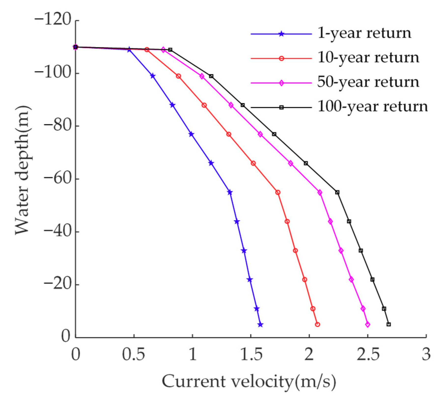
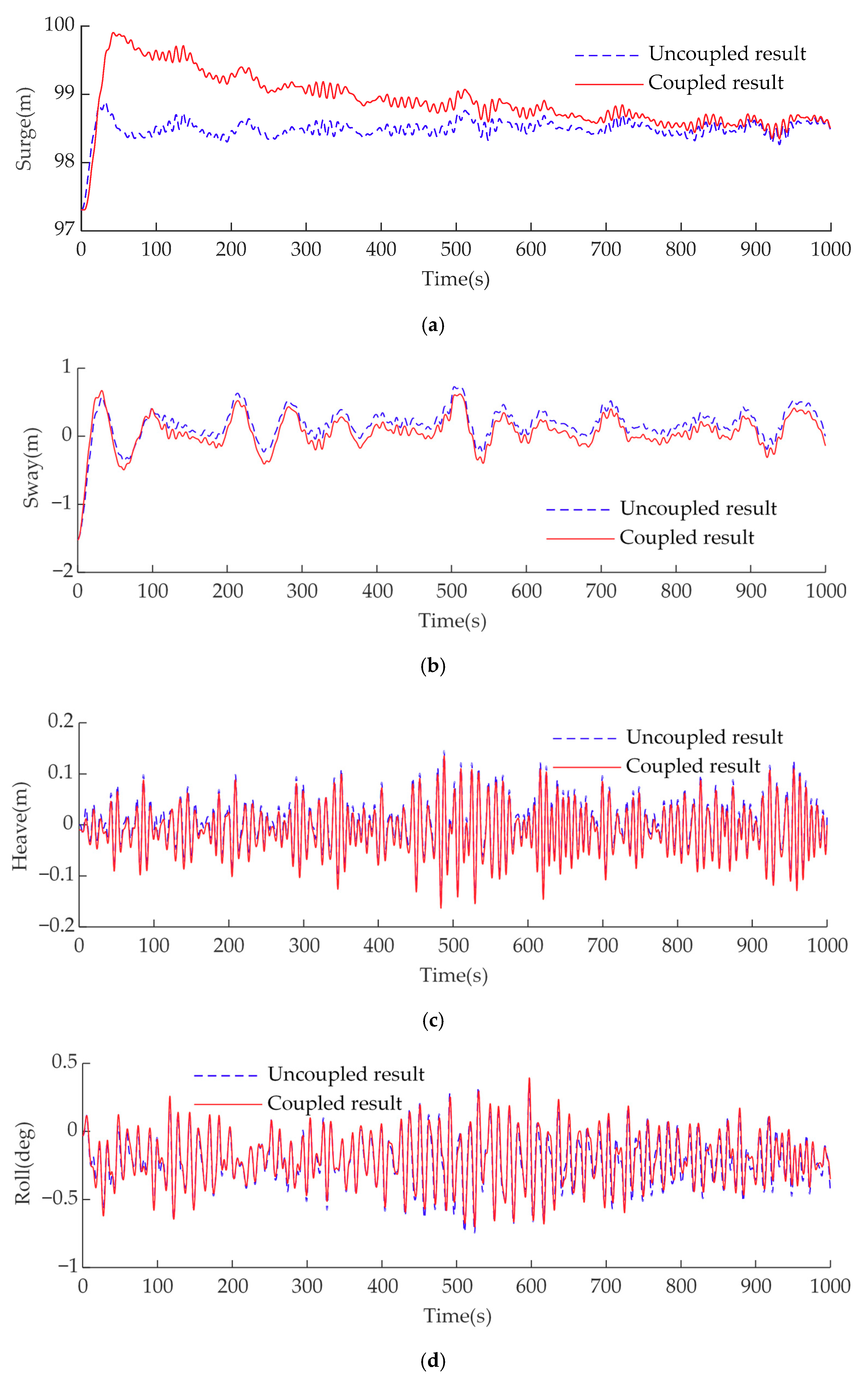
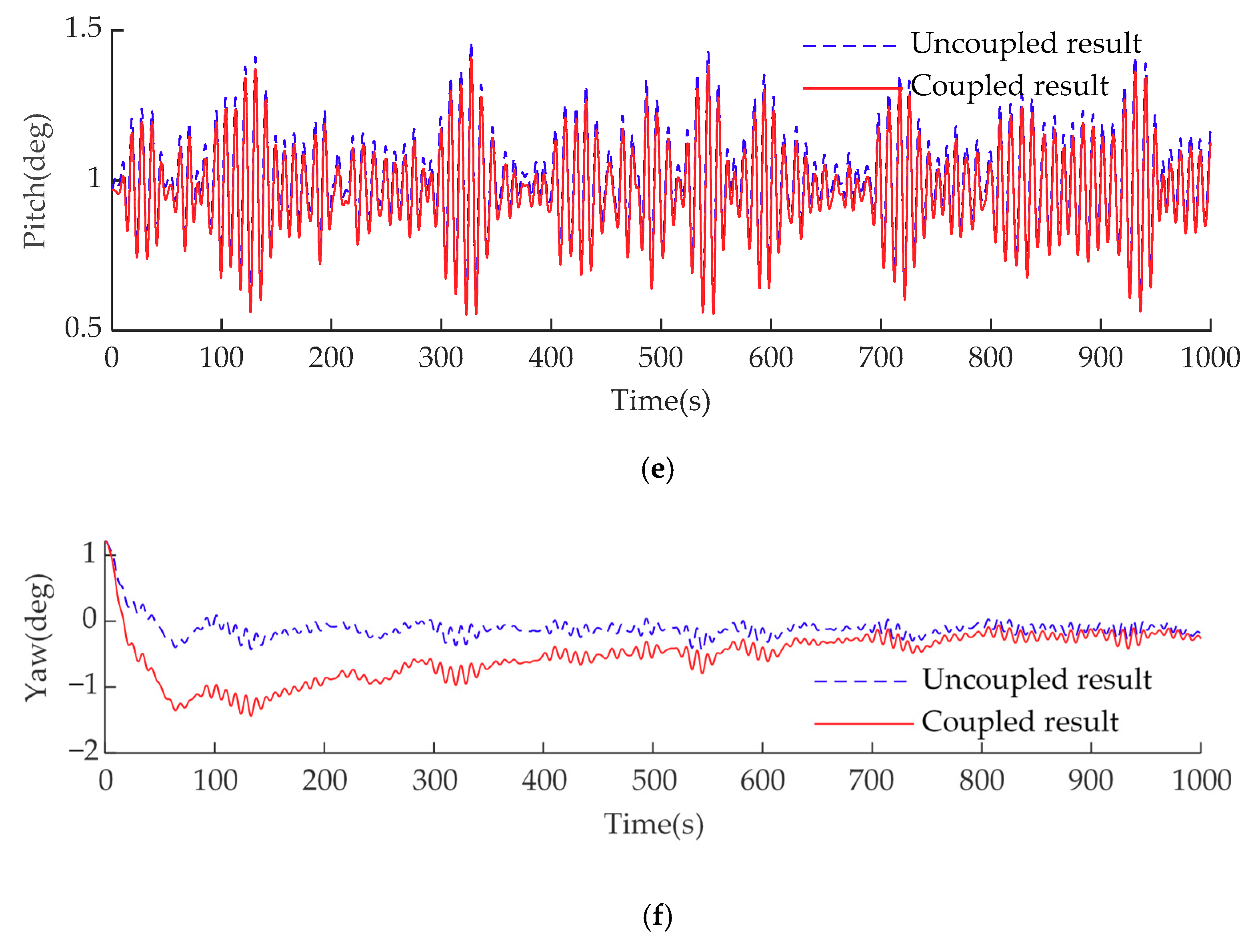
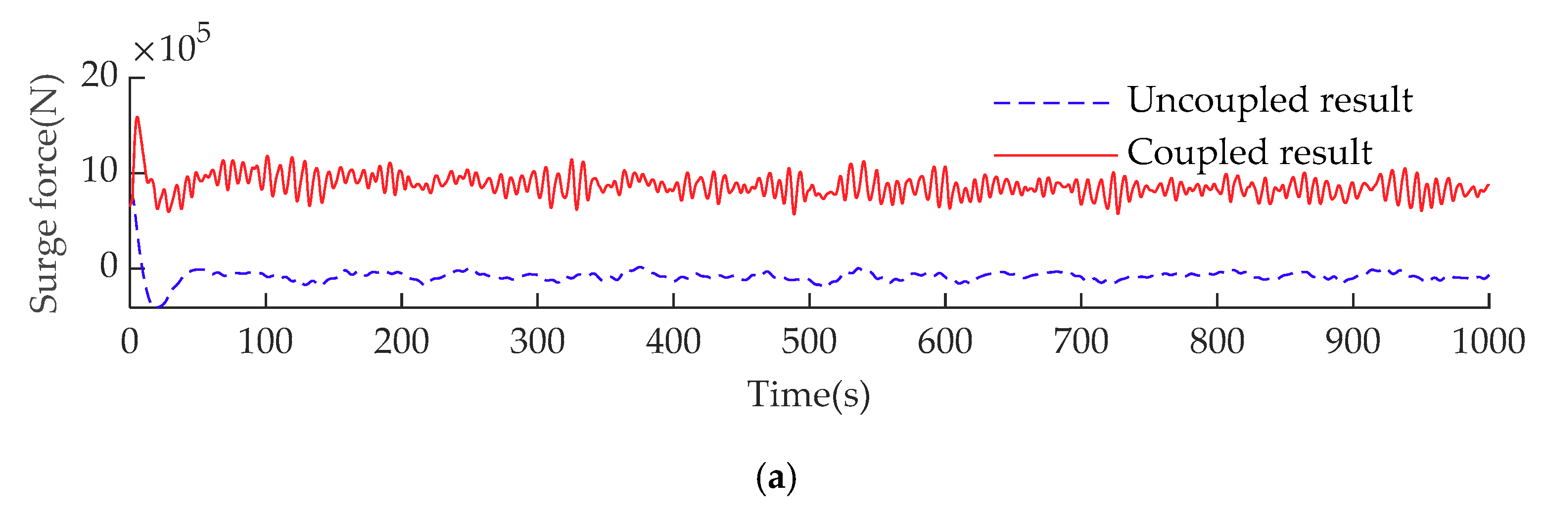
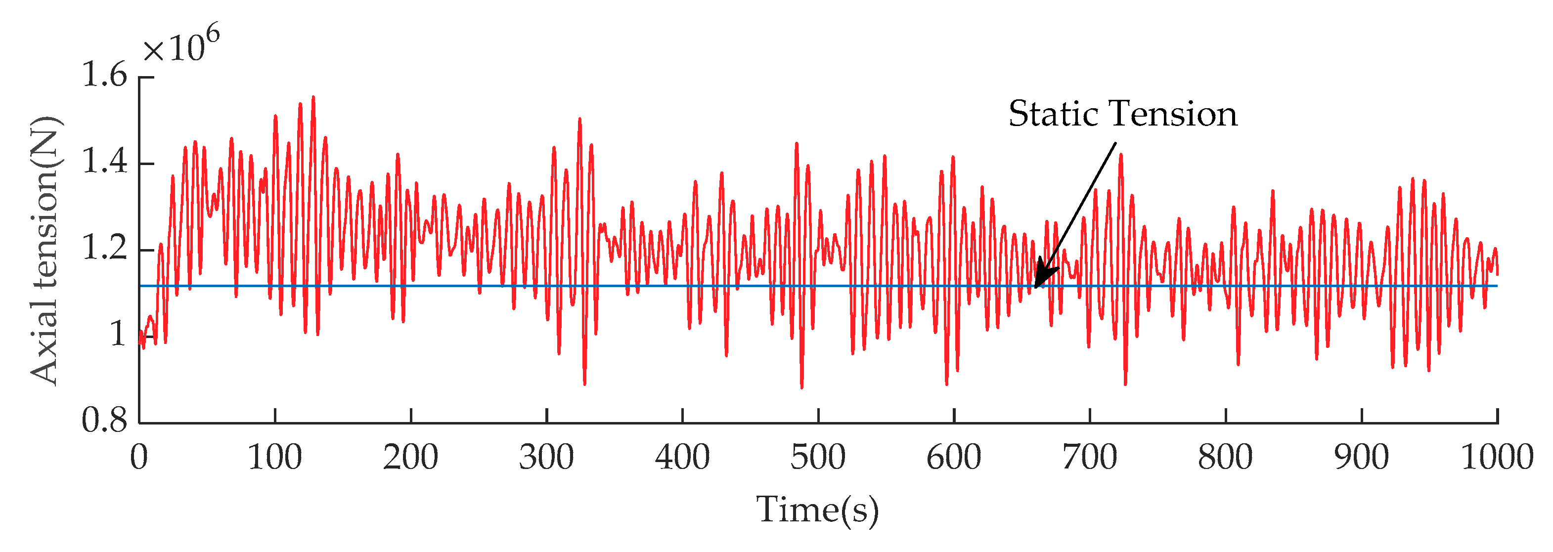
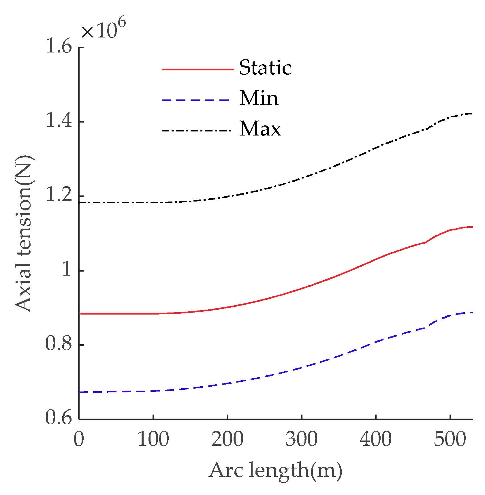
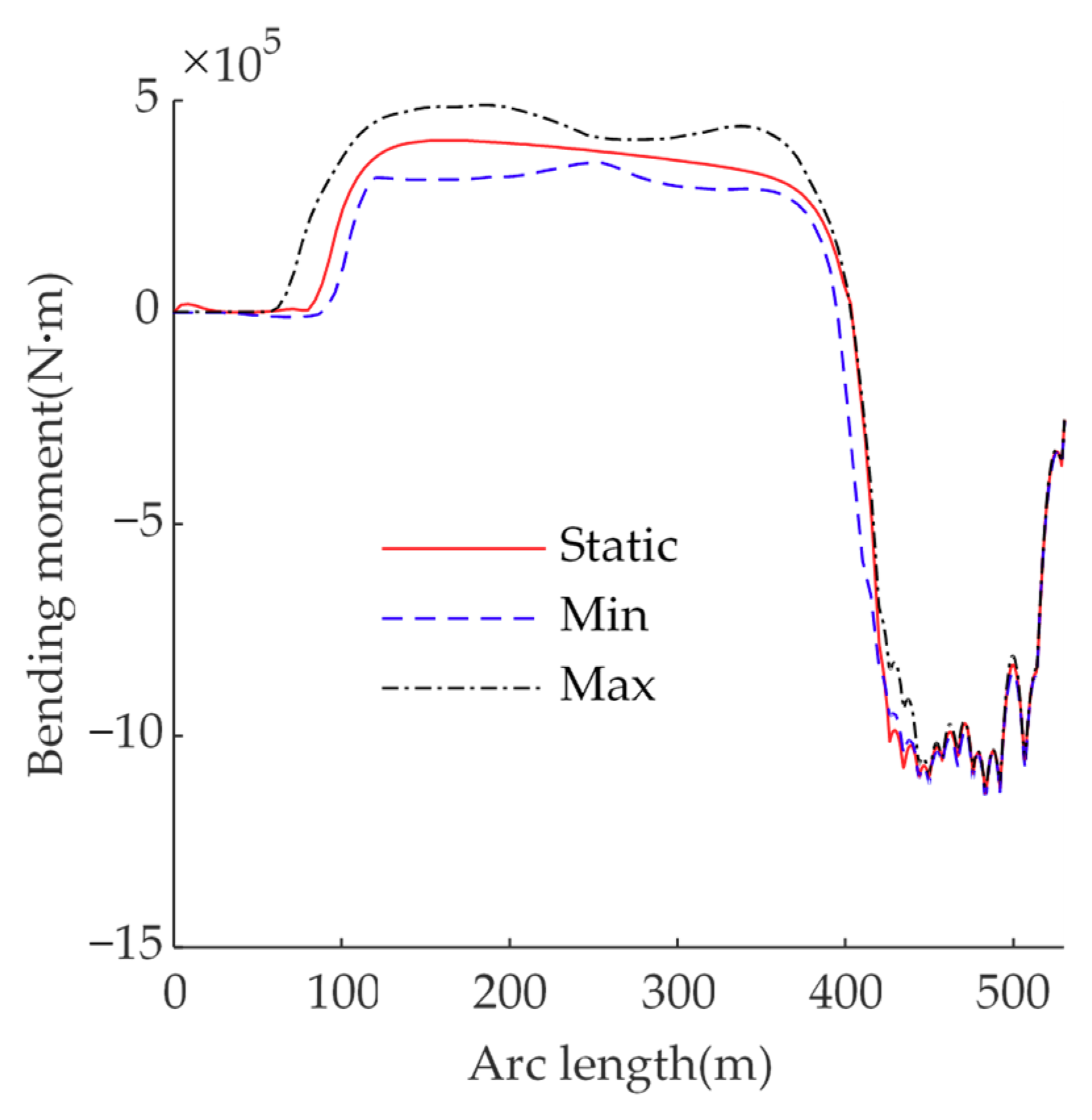
4.2. Coupled Dynamic Pipelaying Analysis Results

The velocity values of the currents within the oil and gas fields of Pingbei-Huangyan were obtained from field measurements. Figure 11 illustrates the differences in current velocity for various annual return periods and water depths. The current velocity data for 1-year return periods at varying water depths were used in the dynamic analysis. The current direction was assumed to be coincident with the heading of the pipelaying vessel.

Table 4. Environmental parameters for the hydrodynamic basin test.

Hs(m)	Tp(s)	$\mathit{\gamma }$	Vw(m/s)	$\mathit{\alpha }$ (°)
1.5	8.2	3.3	9	45

shows the environmental parameters for the hydrodynamic basin test for significant wave height (H_s), peak period peak (T_p), enhancement factor ($\gamma$), mean wind speed (V_w), and wave direction ($\alpha$). The API (American Petroleum Institute) spectrum model was used to calculate the wind speed acting on the vessel.

The hydrodynamic parameters used in the analysis, the drag coefficient, and the added mass coefficient are presented in

Table 5. Drag and added mass coefficients for the pipeline dynamic analysis.

Items	Value
Drag Coefficient	1.2
Added Mass Coefficient	1

[34].

The initial vessel position was determined (97.3 m, −1.52 m) and the heading angle was 1.22°. The PID controller was switched on and propelled the vessel to the desired surface reference position (98.5 m, 0 m) with a specified heading angle of 0°. The simulation time was 1000 s and the simulation step size was 0.1 s. Figure 12 shows the random wave elevation time history curve in 1000 s, which contains the maximum wave height (2.668 m) at the global time of 497.8 s.

To investigate the S-laying pipeline and DP coupling effect on the results of thruster force allocation, the coupled and decoupled simulations of the dynamic response of the pipelaying system were performed with identical initial conditions. Six degrees of freedom for the vessel motion are presented in Figure 13.

As shown in Figure 13a for surge, the vessel quickly reaches the target position of 98.5 m from the initial position 97.3 m in the uncoupled result. However, in the coupled result, the process takes longer, and the vessel goes through a larger deviation to 99.91 m before it approaches the target position of 98.5 m; this is because of the effect of pipeline forces.

A comparison between coupling and uncoupling for the sway direction is shown in Figure 13b. It can be seen that in both uncoupled and coupled results, the vessel approaches the target position 0 m in a short time, and that sway is slightly less than 1 m around the target position. Furthermore, the dynamic motion that takes coupling into account is slightly smaller than the dynamic motion that does not consider coupling.

Figure 13c,d show that the time histories of coupled results in the heave and roll directions closely follow the uncoupled results. However, the coupled result in the pitch direction is smaller than the uncoupled result, as shown in Figure 13e. This is due to the influence of the pipeline on the vessel stern.

Figure 13f shows that for the yaw direction, the vessel gets to the target position of 0° from its initial position 1.22° in a short time in the uncoupled result, while it takes longer in the coupled result to get to the same position. In addition, the deviation in the coupled result reaches −1.44 m as the vessel approaches the target position. This is much larger than for the uncoupled result.

As shown in Figure 14, the thrust force required under coupling conditions is much greater than that under uncoupling conditions. This is especially true for the surge force shown in Figure 14a, where only a small thrust force is required by the DP system to maintain the thruster’s position when the coupling effect is not considered. When the coupling effect is considered, the total thrust force required increases to 1590 kN. It can be seen from Figure 14b that the difference in thrust force for coupling and without coupling is small in the sway direction. This small difference is the result of the pipeline being in the same direction as the pipelaying vessel. Thus, coupling has less impact on the sway direction force than on the surge direction force. To maintain the pipelaying vessel’s heading and position, the torsional moment in the heading direction of the pipelaying vessel when coupling is considered is 1.3 times the torsional moment when coupling is not considered, as illustrated in Figure 14c.

The time histories for the pipeline top tension force are presented in Figure 15. The dynamic maximum pipeline tension is 1556 kN at the global time of 128 s, which is 39.24% higher than the static tension force (1117.5 kN). The dynamic minimum pipe tension is 880.5 kN at the global time of 488 s, which is about 29.94% smaller than the static tension force (1117.5 kN). Therefore, the designed tensioner capability has to be significantly higher than the static results, and the pipeline dynamic tension should be considered when planning pipeline installations.

Figure 16 and Figure 17 show the minimum and maximum values of the tension force and bending moment of the pipeline when the pipelaying vessel behaves stably for the period of 700 to 1000 s. As shown in Figure 16, the static axial tension force differs significantly from the maximum and minimum tension forces of the pipeline. The maximum axial tension force of the pipeline is 33.76% larger than the static axial tension force, and the minimum axial tension force of the pipeline is 23.88% smaller than the static tension force. The bending moment of the pipeline (Figure 17) in the stinger area, where the arc length of the pipeline is approximately 427–530 m, exhibits almost no change. The bending moment at the upper curved part, where the arc length of the pipeline is approximately 390–427 m, has a small change when compared with the static bending moment. Then, the bending moment increases gradually at the lower curved part, where the arc length of the pipeline is approximately 50–390 m. These results indicate that the movement of the pipelaying vessel has an influence on the bending moment of the pipeline and a strong influence on the axial tension force.

5. Conclusions

This paper presents a coupled dynamic model of a pipelaying vessel and the pipeline. The model takes into account the combined effects of wave, wind, current, and thruster forces to compute the dynamic motion of the vessel. In addition, current forces and roller contact forces with the pipeline were incorporated to calculate the pipeline’s dynamic configurations, tension forces, and bending moments. The results from the model were verified using results from OrcaFlex software. A demonstration of the model was provided by assessing the placement of 22″ gas export pipelines on the seafloor by the HYSY201 pipelaying vessel in the Pingbei-Huangyan oil and gas fields in the East China Sea. The assessment revealed a significant relationship between the dynamic responses of the pipeline and the pipelaying vessel’s motion. This shows that coupled disturbance models, which can compute the coupled motion of the pipeline and vessel are necessary. The dynamic positioning system should be included while computing the motions of the vessel. The most important influence of the pipeline feedback on the vessel is in the surge and the yaw directions. The total thrusting force increased significantly in the coupled model. The coupled model can be of value in planning offshore pipelaying activities and installation.

References

1. Zhang, Z.; Wang, L.; Ci, H. An apparatus design and testing of a flexible pipe-laying in submarine context. Ocean Eng. 2015, 106, 386–395. [Google Scholar] [CrossRef]
2. Zhou, Y.; Wang, D.; Guo, Y.; Liu, S. The static frictional behaviors of rubber for pipe-Laying operation. Appl. Sci. 2017, 7, 760. [Google Scholar] [CrossRef]
3. Li, Z.; Wang, C.; He, N.; Zhao, D. An overview of deepwater pipeline laying technology. China Ocean Eng. 2008, 22, 521–532. [Google Scholar]
4. Bruschi, R.; Vitali, L.; Marchionni, L.; Parrella, A.; Mancini, A. Pipe technology and installation equipment for frontier deep water projects. Ocean Eng. 2015, 108, 369–392. [Google Scholar] [CrossRef]
5. Wang, F.; Chen, J.; Gao, S.; Tang, K.; Meng, X. Development and sea trial of real-time offshore pipeline installation monitoring system. Ocean Eng. 2017, 146, 468–476. [Google Scholar] [CrossRef]
6. Jensen, G.A. Offshore pipelaying dynamics. Ph.D. Thesis, Norwegian University of Science and Technology, Trondheim, Norway, 2010. [Google Scholar]
7. Plunkett, R. Static bending stresses in catenaries and drill strings. J. Eng. Ind. 1967, 89, 31–36. [Google Scholar] [CrossRef]
8. Dixon, D.A.; Rutledge, D.R. Stiffened catenary calculations in pipeline laying problem. J. Eng. Ind. 1968, 90, 153–160. [Google Scholar] [CrossRef]
9. Brewer, W.V.; Dixon, D.A. Influence of lay barge motions on a deepwater pipeline laid under tension. J. Manuf. Sci. Eng. 1970, 92, 595–604. [Google Scholar] [CrossRef]
10. Gong, S.F.; Chen, K.; Chen, Y.; Jin, W.L.; Li, Z.G.; Zhao, D.Y. Configuration analysis of deepwater S-lay pipeline. China Ocean Eng. 2011, 25, 519–530. [Google Scholar] [CrossRef]
11. Zan, Y.; Yuan, L.; Han, D.; Bai, X.; Wu, Z. Real-time dynamic analysis of J-laying. Chaos Soliton Fract. 2016, 89, 381–390. [Google Scholar] [CrossRef]
12. Gong, S.; Xu, P.; Bao, S.; Zhong, W.; He, N.; Yan, H. Numerical modelling on dynamic behaviour of deepwater S-lay pipeline. Ocean Eng. 2014, 88, 393–408. [Google Scholar] [CrossRef]
13. Orcina Ltd. OrcaFlex Manual Version 10.0e; Orcina Ltd.: Cumbria, UK. Available online: https://www.orcina.com/SoftwareProducts/OrcaFlex/Documentation/index.php (accessed on 18 December 2017).
14. Liang, H.; Yue, Q.; Lim, G.; Palmer, A.C. Study on the contact behavior of pipe and rollers in deep S-lay. Appl Ocean Res. 2018, 72, 1–11. [Google Scholar] [CrossRef]
15. Xie, P.; Zhao, Y.; Yue, Q.; Palmer, A.C. Dynamic loading history and collapse analysis of the pipe during deepwater S-lay operation. Mar. Struct. 2015, 40, 183–192. [Google Scholar] [CrossRef]
16. Jensen, G.A.; Safstrom, N.; Nguyen, T.D.; Fossen, T.I. A nonlinear PDE formulation for offshore vessel pipeline installation. Ocean Eng. 2010, 37, 365–377. [Google Scholar] [CrossRef] [Green Version]
17. Wittbrodt, E.; Szczotka, M.; Maczyński, A.; Wojciech, S. Rigid Finite Element Method in Analysis of Dynamics of Offshore Structures; Springer: Berlin, Germany, 2013. [Google Scholar]
18. Duan, M.; Wang, Y.; Estefen, S.; He, N.; Li, L.; Chen, B. An installation system of deepwater risers by an S-lay vessel. China Ocean Eng. 2011, 25, 139–148. [Google Scholar] [CrossRef]
19. Wang, F.; Luo, Y.; Xie, Y.; Li, B.; Li, J. Practical and theoretical assessments of subsea installation capacity for HYSY 201 laybarge according to recent project performances in South China Sea. In Proceedings of the Offshore Technology Conference; 5–8 May 2014. [Google Scholar]
20. Cummins, W. The Impulse Response Function and Ship motions. Available online: http://dome.mit.edu/bitstream/handle/1721.3/49049/DTMB_1962_1661.pdf?sequence=1 (accessed on 10 May 2015).
21. Newman, J.N. Marine Hydrodynamics; MIT Press: Boston, MA, USA, 2018. [Google Scholar]
22. Ogilvie, T.F. Recent progress toward the understanding and prediction of ship motions. In Proceedings of the 5th Symposium on Naval Hydrodynamics, Bergen, Norway, 10–12 September 1964; pp. 3–80. [Google Scholar]
23. Hasselmann, K.; Barnett, T.; Bouws, E.; Carlson, H.; Cartwright, D.; Enke, K.; Ewing, J.; Gienapp, H.; Hasselmann, D. Measurements of Wind-Wave Growth and Swell Decay during the Joint North Sea Wave Project (JONSWAP); Technical Report; Deutches Hydrographisches Institut: Heidelberg, Germany, January 1973. [Google Scholar]
24. Lee, C.-H.; Newman, J.N. WAMIT User Manual; Versions 6.3, 6.3PC, 6.3S, 6.3S-PC; WAMIT Inc.: Chestnut Hill, MA, USA, 2006. [Google Scholar]
25. Forum, O.C.I.M. Prediction of Wind and Current Loads on VLCCs, 2nd ed.; Witherby & Co.: London, UK, 1994. [Google Scholar]
26. Choi, J.W.; Park, J.J. A Study on the Effects of Wind Load on the DP Capability. In Proceedings of the Twenty-fourth International Ocean and Polar Engineering Conference, Busan, Korea, June 15–20 2014. [Google Scholar]
27. SINTEF Ocean. SIMO 4.12.2 Theory Manual. Available online: https://www.sintef.no/globalassets/upload/marintek/pdf-filer/sofware/simo.pdf (accessed on 10 June 2018).
28. Yang, X.; Sun, L.; Chai, S. Time Domain Simulation of a Dynamic Positioning Deepwater Semisubmersible Drilling Platform. In Proceedings of the ASME 2014 33rd International Conference on Ocean, Offshore and Arctic Engineering, San Francisco, CA, USA, 8–13 June 2014; pp. V08AT06A021–V008AT006A021. [Google Scholar]
29. Malvern, L.E. Introduction to the Mechanics of a Continuous Medium; Prentice Hall, Inc.: Englewood, NJ, USA, 1969. [Google Scholar]
30. SINTEF Ocean. RIFLEX 4.12.2 Theory Manual. Available online: https://www.sintef.no/globalassets/upload/marintek/pdf-filer/sofware/riflex.pdf (accessed on 10 June 2018).
31. Morison, J.; Johnson, J.; Schaaf, S. The force exerted by surface waves on piles. J. Pet. Technol. 1950, 2, 149–154. [Google Scholar] [CrossRef]
32. Faltinsen, O. Sea Loads on Ships and Offshore Structures; Cambridge University Press: Cambridge, UK, 1993; Volume 1. [Google Scholar]
33. Gong, S.; Xu, P. The influence of sea state on dynamic behaviour of offshore pipelines for deepwater S-lay. Ocean Eng. 2016, 111, 398–413. [Google Scholar] [CrossRef]
34. Wilson, B.W. Characteristics of Anchor Cables in Uniform Ocean Currents; Texas A & M University: College Station, TX, USA, 1960. [Google Scholar]
Figure 1. Schematic diagram of S-laying pipeline installation.
Processes 06 00261 g001
Figure 2. The HYSY201 operating at sea.
Processes 06 00261 g002
Figure 3. Jonswap spectra for four sea states.
Processes 06 00261 g003
Figure 4. The current coefficients for HYSY201.
Processes 06 00261 g004
Figure 5. The wind coefficients for HYSY201.
Processes 06 00261 g005
Figure 6. The arrangement and position of the HYSY201 thrusters.
Processes 06 00261 g006
Figure 7. The particle motion during deformation.
Processes 06 00261 g007
Figure 8. Stinger for S-laying operations: (a) articulated stinger of the HYSY201 and (b) the pipeline in contact with the stinger roller.
Processes 06 00261 g008
Figure 9. Solution procedure for the coupled model.
Processes 06 00261 g009
Figure 10. Comparison between the present model results and OrcaFlex simulations: (a) configurations; (b) tension forces; and (c) bending moments.
Processes 06 00261 g010aProcesses 06 00261 g010b
Figure 11. The variation of the current velocity at different water depths.
Processes 06 00261 g011
Figure 12. The time history of the wave elevation.
Processes 06 00261 g012
Figure 13. Time histories for the vessel’s six degrees of freedom of motion for uncoupled and coupled results: (a) Surge, (b) Sway, (c) Heave, (d) Roll, (e) Pitch, and (f) Yaw.
Processes 06 00261 g013aProcesses 06 00261 g013b
Figure 14. Dynamic total force thrust for uncoupled and coupled results: (a) Surge direction force; (b) Sway direction force; and (c) Yaw direction moment.
Processes 06 00261 g014aProcesses 06 00261 g014b
Figure 15. Time histories for the pipeline top tension force.
Processes 06 00261 g015
Figure 16. Comparison of axial tension forces.
Processes 06 00261 g016
Figure 17. Comparison of bending moments.
Processes 06 00261 g017