A Long-Short Term Memory Recurrent Neural Network Based Reinforcement Learning Controller for Office Heating Ventilation and Air Conditioning Systems

Abstract
:1. Introduction
1.1. Motivation and Background
1.2. Previous Work
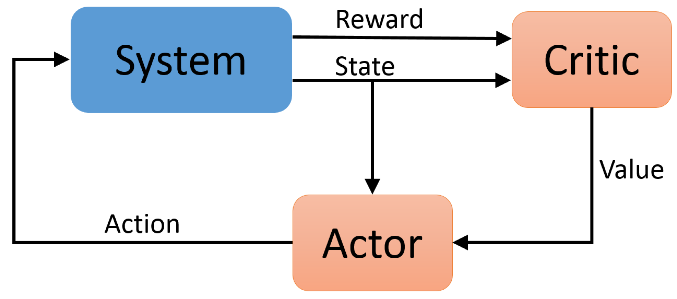
- The use of a model-free, actor-critic method that allows for a stochastic policy and continuous controller output. The use of a critic as a variance-reducing baseline also improves upon the sample efficiency.
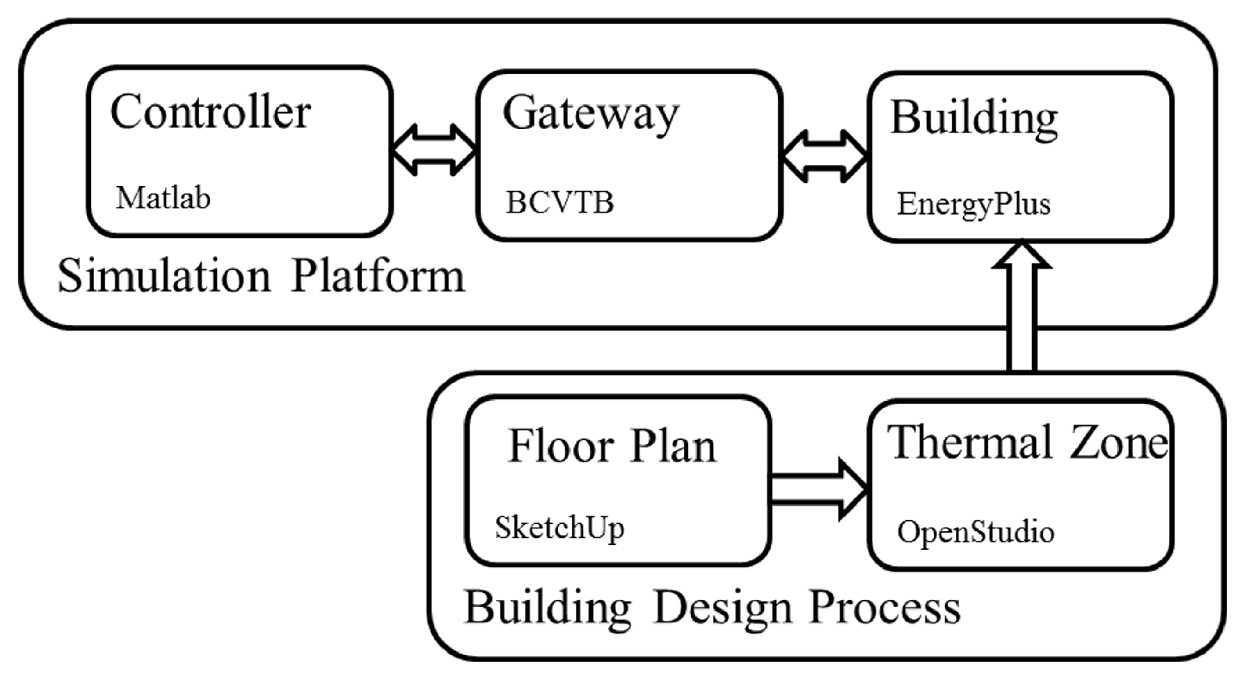
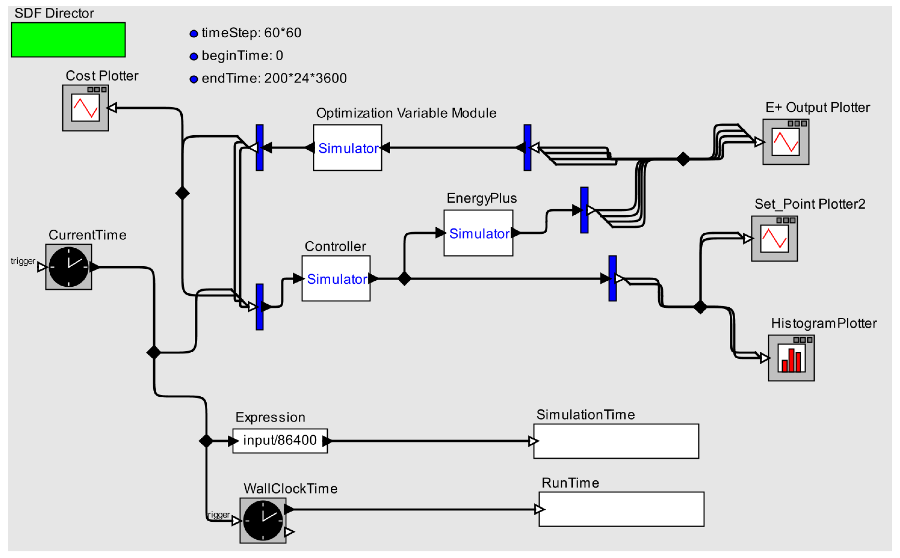
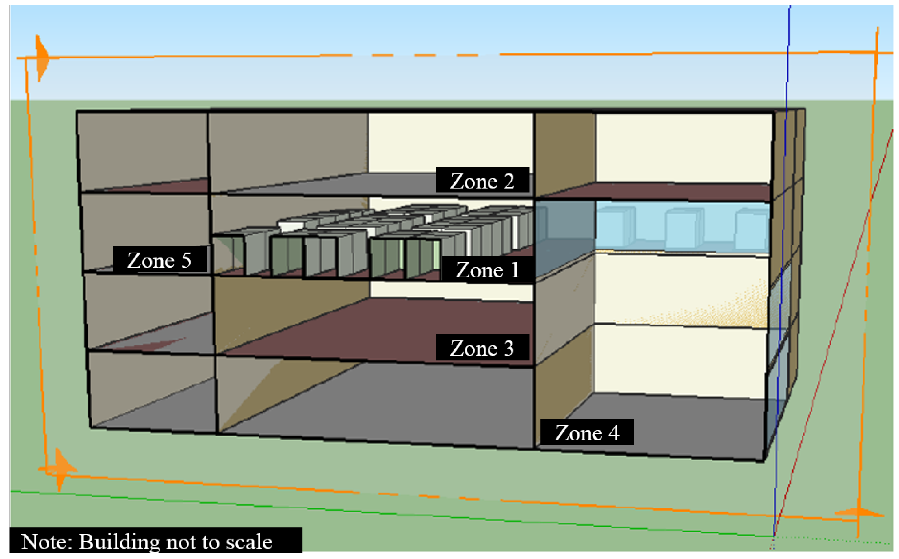
2. Platform Setup
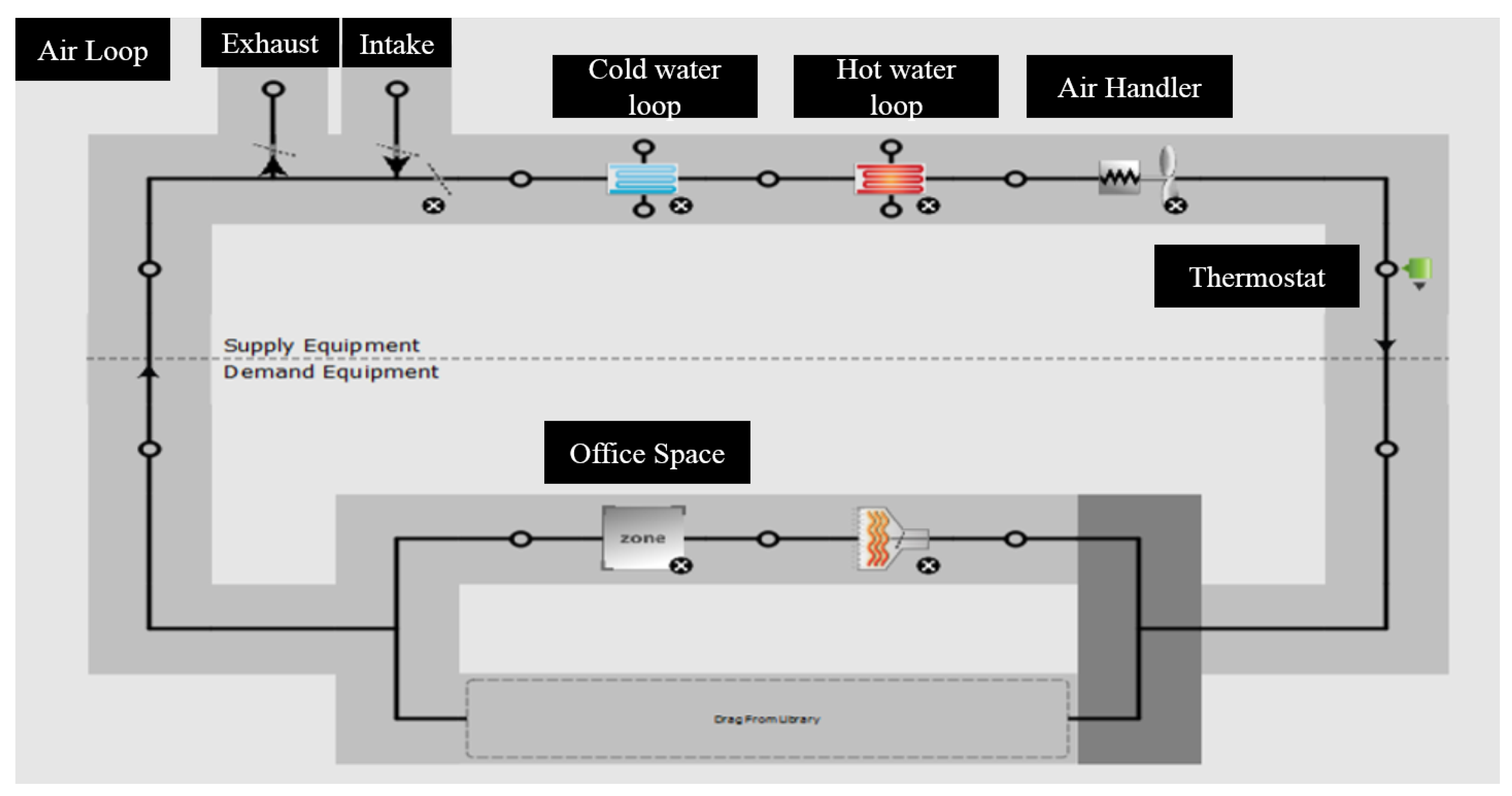
2.1. EnergyPlus
2.2. BCVTB
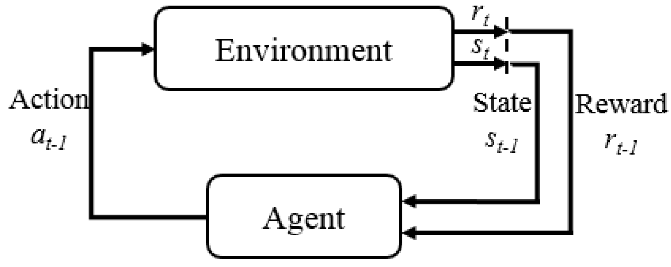
3. Deep Reinforcement Learning
3.1. Introduction
3.2. Markov Decision Processes and Value Functions
- : state space, the set of all possible states of the environment.
- : action space, the set of all possible actions, from which the agent selects one at every time step.
- : reward, a scalar reward emitted by the environment at every time step.
- : policy, which maps from state observation s to action a. Typically, stochastic policies are used; however, deterministic policies can also be specified.
- : transition probability distribution, which specifies the one-step dynamics of the environment, the probability that the environment will emit reward r and transition to subsequent state from being in state s and having taken action a.
3.3. Policy Gradient
3.4. Actor-Critic Methods
| Algorithm 1 Monte Carlo on policy actor-critic. |
Require: Initialize policy with parameters and value critic with parameters
|
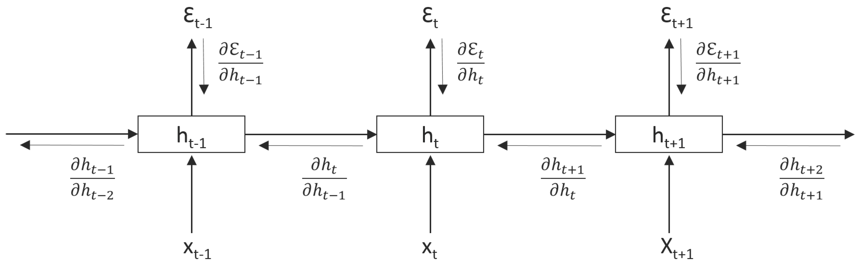
4. Recurrent Neural Networks
4.1. Vanilla Recurrent Neural Network
- The same layer weights and are re-used for each step of computation throughout the sequential data
- An RNN is similar to a deep feedforward neural network when unrolled through time. The depth will be of the length of the sequential data, and for each layer, the weights are the same
4.2. Vanishing and Exploding Gradient Problem
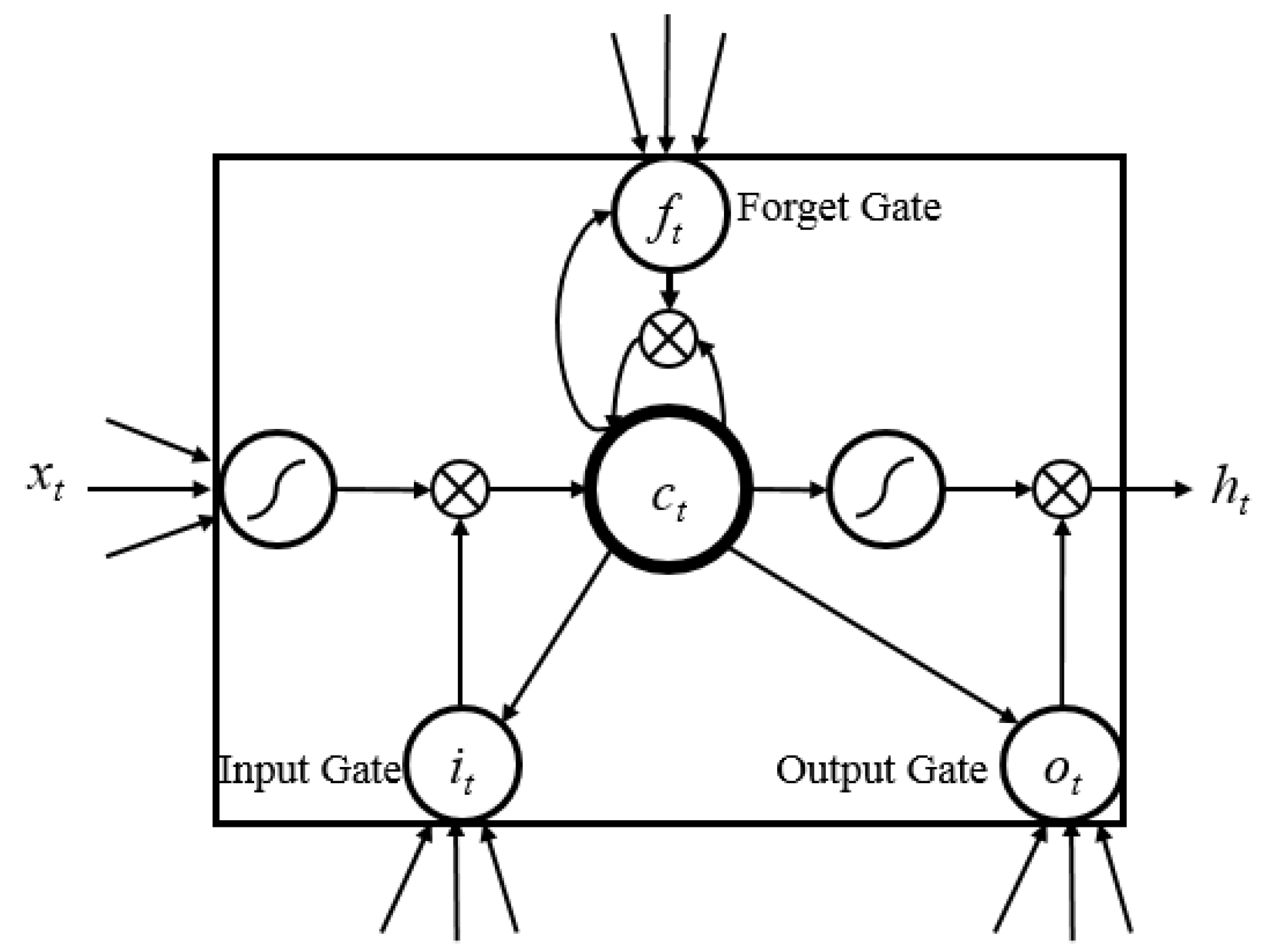
4.3. Long-Short-Term-Memory Recurrent Neural Network
- Learnable gates that modulate the flow of information.
- A persistent cell state that has minimal interactions, providing an easy path for gradient flow during back-propagation.
5. Setup
5.1. Simulation Setup and Parameters
5.2. Reinforcement Learning Controller Design
5.3. Optimization Cost Function Structure
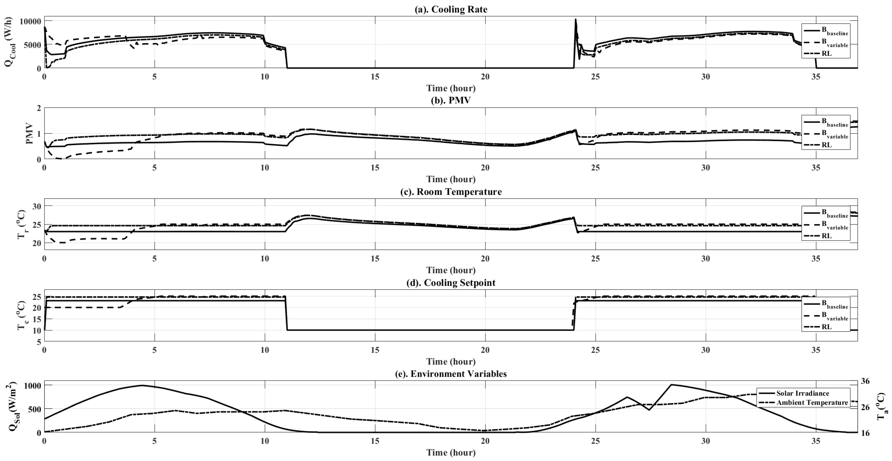
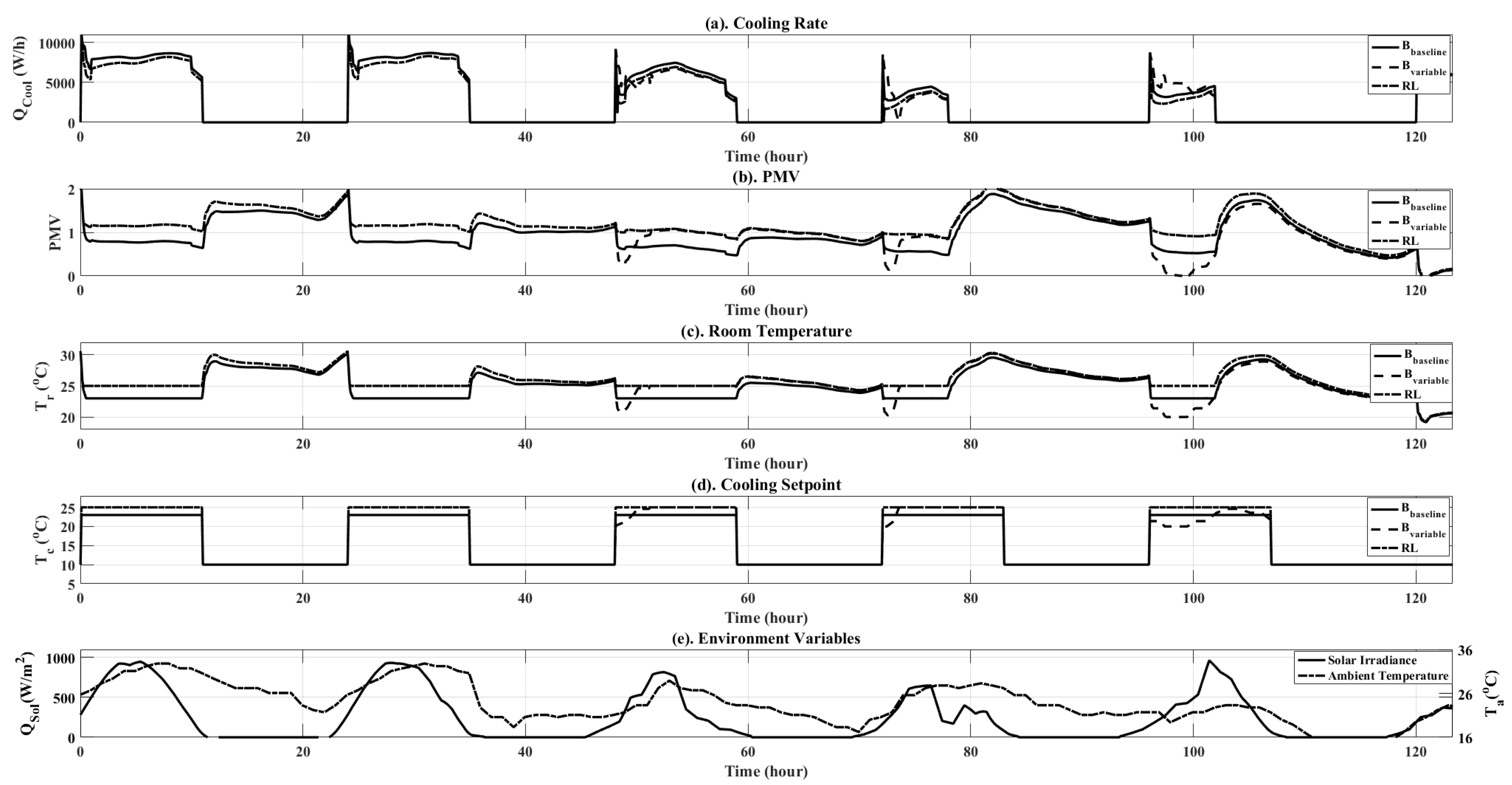
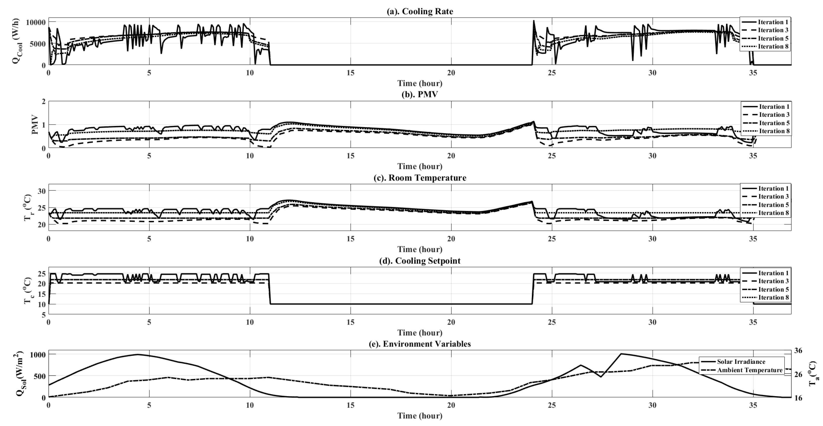
6. Results and Discussion
6.1. Baseline Setup
6.2. RL Training Phase
7. Conclusions
Acknowledgments
Author Contributions
Conflicts of Interest
Abbreviations
| BCVTB | Building Controls Virtual Test Bed |
| BPTT | Back-Propagation Through Time |
| HVAC | Heating Ventilation and Air Conditioning |
| LSTM | Long-Short-Term Memory |
| PMV | Predicted Mean Vote |
| RL | Reinforcement Learning |
| RNN | Recurrent Neural Network |
| TD | Temporal Difference |
| VAV | Variable Air Volume |
References
- International Energy Outlook 2016-Buildings Sector Energy Consumption—Energy Information Administration. Available online: https://www.eia.gov/outlooks/ieo/buildings.cfm (accessed on 25 April 2017).
- Pérez-Lombard, L.; Ortiz, J.; Pout, C. A Review on Buildings Energy Consumption Information. Energ. Build. 2008, 40, 394–398. [Google Scholar] [CrossRef]
- EIA Issues AEO2012 Early Release—Today in Energy—U.S. Energy Information Administration (EIA). Available online: https://www.eia.gov/todayinenergy/detail.php?id=4671 (accessed on 25 April 2017).
- Wallace, M.; McBride, R.; Aumi, S.; Mhaskar, P.; House, J.; Salsbury, T. Energy efficient model predictive building temperature control. Chem. Eng. Sci. 2012, 69, 45–58. [Google Scholar] [CrossRef]
- Široký, J.; Oldewurtel, F.; Cigler, J.; Prívara, S. Experimental analysis of model predictive control for an energy efficient building heating system. Appl. Energ. 2011, 88, 3079–3087. [Google Scholar] [CrossRef]
- Mirinejad, H.; Welch, K.C.; Spicer, L. A review of intelligent control techniques in HVAC systems. In Proceedings of the 2012 IEEE Energytech, Cleveland, OH, USA, 29–31 May 2012; pp. 1–5. [Google Scholar]
- Jun, Z.; Kanyu, Z. A Particle Swarm Optimization Approach for Optimal Design of PID Controller for Temperature Control in HVAC. IEEE 2011, 1, 230–233. [Google Scholar]
- Bai, J.; Wang, S.; Zhang, X. Development of an Adaptive Smith Predictor-Based Self-Tuning PI Controller for an HVAC System in a Test Room. Energ. Build. 2008, 40, 2244–2252. [Google Scholar] [CrossRef]
- Bai, J.; Zhang, X. A New Adaptive PI Controller and Its Application in HVAC Systems. Energ. Convers. Manag. 2007, 48, 1043–1054. [Google Scholar] [CrossRef]
- Lim, D.; Rasmussen, B.P.; Swaroop, D. Selecting PID Control Gains for Nonlinear HVAC & R Systems. HVAC R Res. 2009, 15, 991–1019. [Google Scholar]
- Xu, M.; Li, S.; Cai, W. Practical Receding-Horizon Optimization Control of the Air Handling Unit in HVAC Systems. Ind. Eng. Chem. Res. 2005, 44, 2848–2855. [Google Scholar] [CrossRef]
- Zaheer-Uddin, M.; Tudoroiu, N. Neuro-PID tracking control of a discharge air temperature system. Energ. Convers. Manag. 2004, 45, 2405–2415. [Google Scholar] [CrossRef]
- Wang, Y.-G.; Shi, Z.-G.; Cai, W.-J. PID autotuner and its application in HVAC systems. In Proceedings of the 2001 American Control Conference (Cat. No.01CH37148), Arlington, VA, USA, 25–27 June 2001; pp. 2192–2196. [Google Scholar]
- Pal, A.; Mudi, R. Self-tuning fuzzy PI controller and its application to HVAC systems. Int. J. Comput. Cognit. 2008, 6, 25–30. [Google Scholar]
- Moradi, H.; Saffar-Avval, M.; Bakhtiari-Nejad, F. Nonlinear multivariable control and performance analysis of an air-handling unit. Energ. Build. 2011, 43, 805–813. [Google Scholar] [CrossRef]
- Anderson, M.; Buehner, M.; Young, P.; Hittle, D.; Anderson, C.; Tu, J.; Hodgson, D. MIMO robust control for HVAC systems. IEEE Trans. Control Syst. Technol. 2008, 16, 475–483. [Google Scholar] [CrossRef]
- Sahu, C.; Kirubakaran, V.; Radhakrishnan, T.; Sivakumaran, N. Explicit model predictive control of split-type air conditioning system. Trans. Inst. Meas. Control 2015. [Google Scholar] [CrossRef]
- Divyesh, V.; Sahu, C.; Kirubakaran, V.; Radhakrishnan, T.; Guruprasath, M. Energy optimization using metaheuristic bat algorithm assisted controller tuning for industrial and residential applications. Trans. Inst. Meas. Control 2017. [Google Scholar] [CrossRef]
- Dong, B. Non-linear optimal controller design for building HVAC systems. In Proceedings of the 2010 IEEE International Conference on Control Applications, Yokohama, Japan, 8–10 September 2010; pp. 210–215. [Google Scholar]
- Greensfelder, E.M.; Henze, G.P.; Felsmann, C. An investigation of optimal control of passive building thermal storage with real time pricing. J. Build. Perform. Simul. 2011, 4, 91–104. [Google Scholar] [CrossRef]
- Kirubakaran, V.; Sahu, C.; Radhakrishnan, T.; Sivakumaran, N. Energy efficient model based algorithm for control of building HVAC systems. Ecotoxicol. Environ. Saf. 2015, 121, 236–243. [Google Scholar] [CrossRef] [PubMed]
- Bunin, G.A.; François, G.; Bonvin, D. A real-time optimization framework for the iterative controller tuning problem. Processes 2013, 1, 203–237. [Google Scholar] [CrossRef]
- Vaccari, M.; Pannocchia, G. A Modifier-Adaptation Strategy towards Offset-Free Economic MPC. Processes 2016, 5, 2. [Google Scholar] [CrossRef]
- Sutton, R.S.; Barto, A.G.; Williams, R.J. Reinforcement learning is direct adaptive optimal control. IEEE Control Syst. 1992, 12, 19–22. [Google Scholar] [CrossRef]
- Anderson, C.W.; Hittle, D.C.; Katz, A.D.; Kretchmar, R.M. Synthesis of reinforcement learning, neural networks and PI control applied to a simulated heating coil. Artif. Intell. Eng. 1997, 11, 421–429. [Google Scholar] [CrossRef]
- Barrett, E.; Linder, S. Autonomous HVAC Control, A Reinforcement Learning Approach. In Machine Learning and Knowledge Discovery in Databases; Lecture Notes in Computer Science; Springer: Berlin, Germany, 2015; pp. 3–19. [Google Scholar]
- Urieli, D.; Stone, P. A Learning Agent for Heat-pump Thermostat Control. In Proceedings of the 2013 International Conference on Autonomous Agents and Multi-agent Systems (AAMAS ’13), International Foundation for Autonomous Agents and Multiagent Systems, Richland, SC, USA, 6–10 May 2013; pp. 1093–1100. [Google Scholar]
- Liu, S.; Henze, G.P. Experimental analysis of simulated reinforcement learning control for active and passive building thermal storage inventory: Part 2: Results and analysis. Energ. Build. 2006, 38, 148–161. [Google Scholar] [CrossRef]
- Liu, S.; Henze, G.P. Evaluation of reinforcement learning for optimal control of building active and passive thermal storage inventory. J. Sol. Energ. Eng. 2007, 129, 215–225. [Google Scholar] [CrossRef]
- Hochreiter, S.; Schmidhuber, J. Long short-term memory. Neural Comput. 1997, 9, 1735–1780. [Google Scholar] [CrossRef] [PubMed]
- Greff, K.; Srivastava, R.K.; Koutník, J.; Steunebrink, B.R.; Schmidhuber, J. LSTM: A search space odyssey. IEEE Trans. Neural Netw. Learn. Syst. 2016, 1–11. [Google Scholar] [CrossRef] [PubMed]
- Fanger, P.O. Thermal comfort. Analysis and applications in environmental engineering. In Thermal Comfort Analysis and Applications in Environmental Engineering; Danish Technical Press: Copenhagen, Denmark, 1970. [Google Scholar]
- Kober, J.; Bagnell, J.A.; Peters, J. Reinforcement learning in robotics: A survey. Int. J. Robot. Res. 2013, 32, 1238–1274. [Google Scholar] [CrossRef]
- Mnih, V.; Kavukcuoglu, K.; Silver, D.; Rusu, A.A.; Veness, J.; Bellemare, M.G.; Graves, A.; Riedmiller, M.; Fidjeland, A.K.; Ostrovski, G. Human-level control through deep reinforcement learning. Nature 2015, 518, 529–533. [Google Scholar] [CrossRef] [PubMed]
- Giannoccaro, I.; Pontrandolfo, P. Inventory management in supply chains: A reinforcement learning approach. Int. J. Prod. Econ. 2002, 78, 153–161. [Google Scholar] [CrossRef]
- Ng, A.Y.; Jordan, M. PEGASUS: A policy search method for large MDPs and POMDPs. In Proceedings of the Sixteenth Conference on Uncertainty in Artificial Intelligence, Stanford, CA, USA, 30 June–3 July 2000; pp. 406–415. [Google Scholar]
- Glynn, P.W. Likelihood ratio gradient estimation for stochastic systems. Commun. ACM 1990, 33, 75–84. [Google Scholar] [CrossRef]
- Sutton, R.S.; McAllester, D.A.; Singh, S.P.; Mansour, Y. Policy gradient methods for reinforcement learning with function approximation. NIPS 1999, 99, 1057–1063. [Google Scholar]
- Schulman, J.; Moritz, P.; Levine, S.; Jordan, M.; Abbeel, P. High-dimensional continuous control using generalized advantage estimation. arXiv, 2015; arxiv:1506.02438. [Google Scholar]
- Krizhevsky, A.; Sutskever, I.; Hinton, G.E. Imagenet classification with deep convolutional neural networks. In Proceedings of the 25th International Conference on Neural Information Processing Systems, Lake Tahoe, NE, USA, 3–6 December 2012; pp. 1097–1105. [Google Scholar]
- Sutskever, I.; Vinyals, O.; Le, Q.V. Sequence to sequence learning with neural networks. In Proceedings of the 27th International Conference on Neural Information Processing Systems, Montreal, QC, Canada, 8–13 December 2014; pp. 3104–3112. [Google Scholar]
- Chen, C.; Seff, A.; Kornhauser, A.; Xiao, J. Deepdriving: Learning affordance for direct perception in autonomous driving. In Proceedings of the IEEE International Conference on Computer Vision, Chile, 7–13 December 2015; pp. 2722–2730. [Google Scholar]


| Hours | Office Occupancy | Equipment Active Schedule |
|---|---|---|
| 01:00 a.m. | 0 | 0 |
| 02:00 a.m. | 0 | 0 |
| 03:00 a.m. | 0 | 0 |
| 04:00 a.m. | 0 | 0 |
| 05:00 a.m. | 0 | 0 |
| 06:00 a.m. | 0 | 0 |
| 07:00 a.m. | 0.5 | 1 |
| 08:00 a.m. | 1.0 | 1 |
| 09:00 a.m. | 1.0 | 1 |
| 10:00 a.m. | 1.0 | 1 |
| 11:00 a.m. | 1.0 | 1 |
| 12:00 p.m. | 0.5 | 1 |
| 01:00 p.m. | 1.0 | 1 |
| 02:00 p.m. | 1.0 | 1 |
| 03:00 p.m. | 1.0 | 1 |
| 04:00 p.m. | 1.0 | 1 |
| 05:00 p.m. | 0.5 | 1 |
| 06:00 p.m. | 0.1 | 1 |
| 07:00 p.m. | 0 | 0 |
| 08:00 p.m. | 0 | 0 |
| 09:00 p.m. | 0 | 0 |
| 10:00 p.m. | 0 | 0 |
| 11:00 p.m. | 0 | 0 |
| 12:00 a.m. | 0 | 0 |
| Iteration Number | PMV Total (Unitless) | Energy Total (W) | Standard Deviation ( W/h) |
|---|---|---|---|
| 1 | 216.70 | 16,717 | 3580 |
| 2 | 113.50 | 18,079 | 3480 |
| 3 | 105.60 | 18,251 | 3500 |
| 4 | 262.00 | 15,398 | 3070 |
| 5 | 132.12 | 17,698 | 3450 |
| 6 | 211.30 | 16,300 | 3240 |
| 7 | 211.50 | 16,310 | 3240 |
| 8 | 211.30 | 16,298 | 3228 |
| Control Type | PMV (Unitless) | Energy Total (W) |
|---|---|---|
| Ideal PMV | 190.00 | 16,676 |
| Variable Control | 250.00 | 15,467 |
| RL Control | 211.3 | 16,298 |
| Control Type | PMV Total (Unitless) | Energy Total (W) |
|---|---|---|
| Ideal PMV | 510 | 42,094 |
| Variable Control | 660 | 38,536 |
| RL Control | 558 | 39,978 |
© 2017 by the authors. Licensee MDPI, Basel, Switzerland. This article is an open access article distributed under the terms and conditions of the Creative Commons Attribution (CC BY) license (http://creativecommons.org/licenses/by/4.0/).
Share and Cite
Wang, Y.; Velswamy, K.; Huang, B. A Long-Short Term Memory Recurrent Neural Network Based Reinforcement Learning Controller for Office Heating Ventilation and Air Conditioning Systems. Processes 2017, 5, 46. https://doi.org/10.3390/pr5030046
Wang Y, Velswamy K, Huang B. A Long-Short Term Memory Recurrent Neural Network Based Reinforcement Learning Controller for Office Heating Ventilation and Air Conditioning Systems. Processes. 2017; 5(3):46. https://doi.org/10.3390/pr5030046
Chicago/Turabian StyleWang, Yuan, Kirubakaran Velswamy, and Biao Huang. 2017. "A Long-Short Term Memory Recurrent Neural Network Based Reinforcement Learning Controller for Office Heating Ventilation and Air Conditioning Systems" Processes 5, no. 3: 46. https://doi.org/10.3390/pr5030046
APA StyleWang, Y., Velswamy, K., & Huang, B. (2017). A Long-Short Term Memory Recurrent Neural Network Based Reinforcement Learning Controller for Office Heating Ventilation and Air Conditioning Systems. Processes, 5(3), 46. https://doi.org/10.3390/pr5030046