Abstract
We have developed a closed-loop, high-throughput system that applies electrical stimulation and optical recording to facilitate the rapid characterization of extracellular, stimulus-evoked neuronal activity. In our system, a microelectrode array delivers current pulses to a dissociated neuronal culture treated with a calcium-sensitive fluorescent dye; automated real-time image processing of high-speed digital video identifies the neuronal response; and an optimized search routine alters the applied stimulus to achieve a targeted response. Action potentials are detected by measuring the post-stimulus, calcium-sensitive fluorescence at the neuronal somata. The system controller performs directed searches within the strength–duration (SD) stimulus-parameter space to build probabilistic neuronal activation curves. This closed-loop system reduces the number of stimuli needed to estimate the activation curves when compared to the more commonly used open-loop approach. This reduction allows the closed-loop system to probe the stimulus regions of interest in the multi-parameter waveform space with increased resolution. A sigmoid model was fit to the stimulus-evoked activation data in both current (strength) and pulse width (duration) parameter slices through the waveform space. The two-dimensional analysis results in a set of probability isoclines corresponding to each neuron–electrode pair. An SD threshold model was then fit to the isocline data. We demonstrate that a closed-loop methodology applied to our imaging and micro-stimulation system enables the study of neuronal excitation across a large parameter space.
1. Introduction
The application of stimulus-evoked activity to characterize neuronal systems is a powerful analysis tool that dates to the 19th-century identification of functional areas of the brain []. Electrical stimulation has since become ubiquitous for research applications such as mapping cortical regions associated with behavioral outputs and uncovering cortical processing mechanisms [,,,,]. Additionally, in vitro studies to investigate the input-output relationship of stimulus-evoked neuronal activity can provide access to the instantaneous response probability of a neuron []. Quantifying the likelihood that a neuron will fire an action potential in response to a given stimulus pulse leads to system designs with greater control over the evoked population activity. Along these lines, Keren and Marom [] investigated the control response features, including probability and latency, of cells responding to a stimulus. They used closed-loop control to deliver stimuli designed to clamp a population firing rate to arbitrary activation probability levels, including a sinusoidal probability pattern. All of these studies use stimulation as a means of understanding neuronal activation properties.
Multidimensional stimulus waveforms offer new approaches for the improvement of stimulus-based control. Specifically, for cathodic extracellular stimulus pulses comprising a stimulus current, or strength, and a stimulus pulse width, or duration, there is a threshold of activation described by the strength-duration (SD) curve [,]. The SD paradigm sees use in both experimental and modeling studies of neuronal activation [,,,,,]. While clinical applications require the use of charge-balanced stimuli, researchers are free to use a variety of stimulus pulse shapes in vitro to explore stimulus-evoked neuronal activation. Some experimentalists prefer to use voltage-controlled stimulus pulses, such as the activation study of Wallach et al. [], however, monophasic cathodic current-controlled pulses eliminate the dependence of a stimulus on the electrode impedance because, regardless of impedance variation across electrode arrays, the current delivered can be consistent. In another study, Mahmud and Vassanelli [] utilize a variety of sinusoidal stimuli to modulate neuronal activation. While the SD curve is rarely applied to probabilistic models of neuronal activation because of the common simplifying assumption that the SD curve describes a single activation threshold, the use of a cathodic current pulse allows the SD curve to be explicitly defined across probabilities. The activation probability of a neuron, like that of the population activation defined in Wallach et al. [], is more accurately modeled with a gradating activation probability. Modeling a gradating activation probability requires that a different SD curve be used to describe each probability level, which requires estimation of a large number of activation parameters.
The complexity of characterizing a multidimensional parameter space—even a 2-D space—invites closed-loop (CL) approaches to stimulus design. Automated CL methodologies are inherently more efficient in collecting the most informative data from each stimulus trial, resulting in faster characterization of neuronal activation [,,,,]. Newman et al. [] developed a robust system of closed-loop stimulation and recording to investigate the clamping of a neuronal population firing rate, enabling a robot to move through space in a direction which is guided by the recorded activity, and real-time seizure intervention in freely moving rats. The investigations were made possible by the closed-loop design of the system, including the incorporation of optogenetic control in an in vitro culture []. Improvements in spatiotemporal resolution enable better stimulus control, and Vassanelli et al. [] achieved bi-directional communication between their stimuli and a neuronal population. Additionally, in vivo closed-loop stimulation is showing great promise in improving stimulus efficacy for treatment of epilepsy using interventional optogenetic stimulation [] and closed-loop deep brain stimulation (DBS) for the treatment of Parkinson’s Disease []. Schiller and Bankirer [] demonstrated antiepileptic effects of closed-loop electrical stimulation to neocortical brain slices, in vitro. Weihberger et al. [] delivered closed-loop stimulation to in vitro cultures of neurons to quantify the mechanisms responsible for network spontaneous activity and stimulus response. In many of these applications, CL methodology was instrumental in allowing researchers to improve the efficacy of their stimulation paradigms to treat disorder. Complementary to direct clinical applications is the use of CL tools to characterize neuronal response to stimulation to improve our understanding of the direct action of stimuli.
We present an automated, real-time, closed-loop system that combines electrical stimulation and optical imaging for rapid exploration of the extracellular electrical stimulus waveform space. This technology and software methodology enables us to describe the probabilistic activation of a neuron in response to a stimulus. Stimulus response is measured through optical imaging of molecular probes, and the evoked response is used to calculate the next stimulus. Automated closed-loop stimulation, with optical imaging in vitro, grants the ability to improve the mapping from stimulus to excitation. Optical recording provides a means to directly measure stimulus-evoked activity [] at the individual neuron and record the spatial organization of activated neurons. By developing a more efficient characterization of the large parameter space, we can then rapidly extract single-parameter activation curves and two-parameter strength-duration curves for an arbitrary neuron. We use online data analysis for stimulus optimization to create smarter goal-directed stimuli and, additionally, by reducing the number of stimuli needed for understanding a particular neuron’s activation curve, light exposure is minimized within an experiment to reduce phototoxicity and photobleaching. We use a model-driven CL approach which fits a sigmoid to a probabilistic neuronal activation curve. Our stimuli target the transition region, in which a neuron transitions from low to high firing probability. This enables the routine to converge on the model parameters more quickly when compared to open-loop approaches. Closed-loop optimization for determining the stimulus at each iteration allows for the characterization of the stimulus pulse space by rapidly homing in on the relevant parameters. While CL experimentation grows increasingly popular across research fields, the application of CL stimulation and recording to neurons in vitro within a modular system can allow for high-throughput experimentation that reduces experimental time and permits the exploration of many different stimulus paradigms for targeted neuronal stimulation. Our system allows us to model both neuronal activation and strength-duration curves, which enables the design of stimuli that may target particular neuronal populations.
2. Methods
We designed a closed-loop system (Figure 1) for optimizing stimulus pulse parameters based on a model of neuronal activation and an experimental goal. The system comprises hardware and software components that select and deliver stimuli, which are designed to evoke a particular neuronal response. Each measured response is used to refine the model and the next stimulus is automatically chosen. The modular design, which separates data collection from both data analysis and decision making, enables the user to define a model function and a variety of output measures to ask and answer a multitude of questions. Each section of the system is described in more detail below.
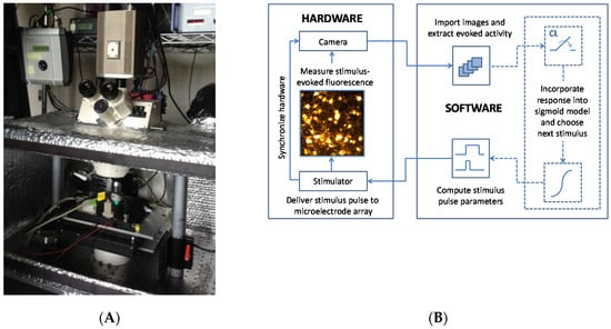
Figure 1.
The closed-loop system of electrical stimulation, optical recording, automated image analysis and activation curve modeling. (A) A photograph of the system apparatus is shown. The camera is mounted atop the microscope with an inline piezoelectric actuator connected to the 20× objective for high-precision focal plane adjustments. LED fluorescence excitation is digitally controlled using the TLC001 current controller eliminating the need for a shutter. The neuronal culture lives atop the microelectrode array (MEA), which is nested inside of the heated Multi Channel Systems preamplifier. Imaging is carried out inside of an enclosure to eliminate ambient light exposure and reduce the effects of other environmental factors including the laboratory heating and ventilation. The preamplifier is housed inside of this “light tight” imaging chamber and interfaces with the external stimulator. (B) Hardware for delivering electrical stimuli and for optically recording evoked responses (left) interfaces directly with the MATLAB-based software system (MATLAB 7.12, The MathWorks Inc., Natick, MA, USA, 2011) (right). The open-loop experimental configuration is depicted with solid arrows. Predefined stimulus pulse parameters are sent to the stimulator for delivery to the MEA. The stimulator supplies synchronizing triggers to the camera, LED, and preamplifier. Fluorescence is evoked at cell somata that fire action potentials in response to the stimulus. This fluorescence signal is captured by the camera with a series of high-speed digital frames. The set of frames is imported into MATLAB and saved to the hard disk using the Micro-Manager library []. In the closed-loop configuration (dotted lines) the neuronal response is used to inform the calculation of the next iteration of stimulus pulse parameters. Digital images are analyzed using custom software to extract stimulus-evoked action potentials. This newly acquired response data is compiled with previous stimulus iterations and the sigmoid activation model is updated to reflect all measured responses. The next stimulus pulse is then chosen to increase the measurement resolution along the slope of the response curve.
2.1. Cortical Cell Culture
The neuronal cultures used in this research ranged in age from 14 DIV to 28 DIV. A phase contrast image of a typical neuronal culture at 14 days in vitro (DIV) is shown in Figure 2. Neurite outgrowth can be observed in between the cell bodies indicating that the cell culture is healthy.
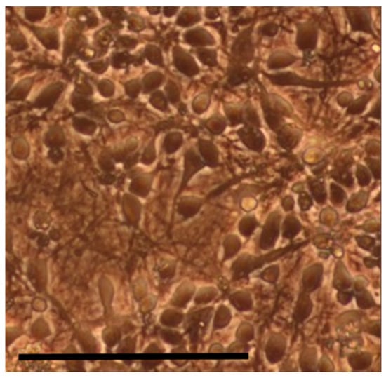
Figure 2.
Dissociated neuronal culture. A phase contrast micrograph of a dissociated rat cortical culture at 14 days in vitro (DIV) illustrates the extent to which the culture has developed. Neurites (axons and dendrites) can be seen in the space between the somata. Scale bar: 100 μm.
Embryonic Day 18 (E18) rat cortices were enzymatically and mechanically dissociated according to Potter and DeMarse []. Cortices were digested with trypsin (0.25% w/Ethylenediaminetetraacetic acid (EDTA)) for 10–12 min, strained through a 40 μm cell strainer to remove clumps, and centrifuged to remove cellular debris. Neurons were re-suspended in culture medium (90 mL Dulbecco’s Modified Eagle’s Medium (Irvine Scientific 9024; Santa Ana, CA, USA), 10 mL horse serum (Life Technologies 1605, 0-122; Carlsbad, CA, USA), 250 μL GlutaMAX (200 mM; Life Technologies 35050-061), 1 mL sodium pyruvate (100 mM; Life Technologies 11360-070) and insulin (Sigma-Aldrich I5500; St. Louis, MO, USA; final concentration 2.5 μg/mL)) and diluted to 3000 cells/μL. Microelectrode arrays (MEAs; Multi Channel Systems 60MEA200/30iR-Ti) were sterilized by soaking in 70% ethanol for 15 min followed by UV exposure overnight. MEAs were treated with polyethylenimine to hydrophilize the surface, followed by three water washes and 30 min of drying. Laminin (10 μL; 0.02 mg/mL; Sigma-Aldrich L2020) was applied to the MEA for 20 min, half of the volume was removed, and 30,000 neurons were plated into the remaining laminin atop the MEA. Cultures were protected using gas-permeable lids [] and incubated at 35 °C in 5% carbon dioxide and 95% relative humidity. The culture medium was fully replaced on the first DIV and then once every four DIV afterwards.
2.2. Electrical Stimulation
Extracellular electrical stimuli were used to elicit neuronal activity. Stimuli were delivered to the neurons using a STG-2004 stimulator and MEA-1060-Up-BC amplifier (Multi Channel Systems). MATLAB (Natick, MA, USA) was used to control all hardware devices, which were synchronized by TTL pulses sent from the stimulator at the beginning of each stimulation loop. In all stimulus iterations, a trigger pulse was first delivered to the camera to begin recording so that background fluorescence levels could be measured. An enable pulse was then delivered to the amplifier, which connected the stimulus channel to a pre-programmed electrode. A single cathodic square current pulse was then delivered to a single electrode centered under the camera field of view. Current-controlled pulses were selected such that the total charge delivered could be consistent across experiments and MEAs, independent of the electrode impedance. Cathodic pulses were chosen because they have been shown to be more effective at evoking a neuronal response, when compared to anodic pulses [].
2.3. Optical Imaging
Automated optical imaging was used to measure the stimulus-evoked neuronal response. All preparation procedures were conducted in the dark to lengthen experiments by minimizing photobleaching and phototoxicity. Culture media was removed and neurons were loaded with Fluo-5F AM (Life Technologies F-14222), a calcium-sensitive fluorescent dye with relatively low binding affinity at a concentration of 9.1 μM in DMSO (Sigma-Aldrich D2650), Pluronic F-127 (Life Technologies P3000MP) and artificial cerebral spinal fluid (aCSF; 126 mM NaCl, 3 mM KCl, 1 mM NaH2PO4, 1.5 mM MgSO4, 2 mM CaCl2, 25 mM D-glucose) with 15 mM HEPES buffer for 30 min at ambient 25 °C and atmospheric carbon dioxide. Before imaging, cultures were rinsed two times with aCSF to remove free dye. Cultures were bathed in a mixture of synaptic blockers in aCSF (15 mM HEPES buffer). This included (2R)-amino-5-phosphonopentanoate (AP5; 50 μM; Sigma-Aldrich A5282), a NMDA receptor antagonist; bicuculline methiodide (BMI; 20 μM; Sigma-Aldrich 14343), a GABAA receptor antagonist; and 6-cyano-7-nitroquinoxaline-2,3-dione (CNQX; 20 μM; Sigma-Aldrich C239), an AMPA receptor antagonist. This mixture was shown to suppress neuronal communication [] to ensure that the recorded neuronal activity was directly evoked by the stimulus. The culture was then kept in the heated amplifier (Multi Channel Systems TC02, 37C) within the imaging chamber. The stage position was calibrated with respect to the desired field of view (FOV) using the electrodes as fiducial markers. A MATLAB GUI was used to automatically position the FOV over the stimulation electrode. During an experiment neurons were illuminated using a light-emitting diode (LED; 500 nm peak power) and LED current source (TLCC-01-Triple LED; Prizmatix) through a 20× immersion objective and a fluorescein isothiocyanate (FITC) filter cube. Evoked activity was optically recorded using a high-speed electron multiplication CCD camera (30 fps; QuantEM 512S; Photometrics, Tucson, AZ, USA), which has a 512 × 512 pixel grid covering a 400 μm × 400 μm area. After an experiment concluded, three aCSF washouts were performed at three minute intervals, the culture media was replaced, and the culture was returned to the incubator.
2.4. Detecting Action Potentials
The data presented in the following studies were taken from four different experiments on different neurons in culture. Each experiment was design to focus on one portion of the experimental system for functional validation. While extracellular stimulation may activate neurons via their neurites [], stimulation can result in antidromic action potentials, which are detectable at the cell body. For each neuron, the measured intensity of a 16 × 16-pixel (12.5 μm × 12.5 μm) field centered on the soma was spatially averaged. Calcium signaling is dynamic and continuous within both neurons and glia associated with a neuronal population; therefore, there exists a low-level fluorescence that can be measured within these cell bodies due to the action of the calcium indicator as a chelator trapped with all cells. However, numerous studies have been published demonstrating the use of calcium indicators to infer neuronal spiking enabled by both the relatively fast and large change in measurable fluorescence at a neuronal cell body immediately following an action potential [,,,].
The relative change in fluorescence, ΔF/F, was calculated by subtracting the baseline (an average of four pre-stimulus frames, 30 fps) from an average of four post-stimulus frames (30 fps) and dividing the difference by the baseline. The post-stimulus frames were defined as those immediately following the delivered stimulus. Two fluorescence traces are shown across time in Figure 3.
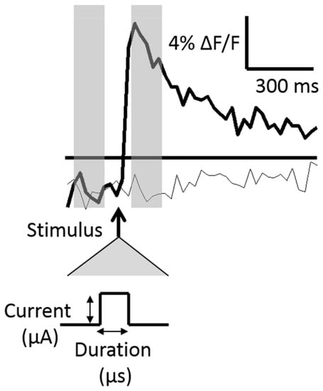
Figure 3.
Stimulus-evoked fluorescence traces. Two traces are shown in which an action potential was evoked in response to the stimulus (bold line) and no action potential was evoked (light line). The stimulus timing with respect to the evoked signal is denoted by the bold arrow and is expanded below to show the two stimulus pulse control variables, the current (μA) and the pulse width, or duration (μs). The fluorescence traces are generated by spatially averaging 16 pixels at a neuron soma. Action potentials were assumed to occur if the post-stimulus change in fluorescence (ΔF/F) was greater than three times pre-stimulus levels (threshold shown as a horizontal bar). The pre-and-post-stimulus fluorescence levels were calculated as a time-average of four frames (represented with transparent gray bars).
Figure 3 shows two traces, one in which an action potential was generated, and one in which no action potential was generated. The standard deviation of the baseline frames was calculated in initial stimulus iterations and used as a measure of the fluorescence noise level. An action potential was assumed to have occurred if the ΔF/F was greater than three times the noise level within a particular neuron.
The average decay time constant of a stimulus-evoked fluorescence curve was 1.5 s. Because of this relatively slow signal decay, the experiment loop time was chosen to be 4.5 s (three decay time constants) to allow the signal sufficient time to return to baseline. The progression of ΔF/F for one neuron over the course of 1140 open-loop stimulus iterations is plotted in Figure 4, which illustrates the evoked signal decay with increasing light exposure. Stimuli were randomly presented from a range of stimulus strengths and durations, such that the neuronal response is mixed throughout the experiment. For the first 200 stimuli, the change in fluorescence resulting from an evoked action potential is unchanging. The signal then subsequently decays with each light exposure.
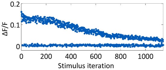
Figure 4.
Evoked fluorescence decays due to photobleaching. The progression of the relative fluorescence change, ΔF/F, is shown across an experiment. A set of 1140 stimuli were applied in random order that spanned the stimulus pulse parameter space. Some of the stimuli evoked action potentials and others did not. The measured ΔF/F, plotted at each stimulus iteration, decays with each light exposure.
2.5. Automated Location of Neuronal Somata
The automated process for locating activated cell bodies is outlined in Figure 5. A single raw image is shown from a series along with the evoked difference image, the processed image gradient and the cells overlaid on the gradient image. In order to first define the population of neurons an automated strategy was employed to locate all cell somata in which activity was evoked in response to a relatively large stimulus. The amplitude of this large current was chosen to evoke as much activity as possible without creating voltages at the electrode that would electrolyze water or creating current densities that could be harmful to those neurons located nearest to the electrode. The first step in the image-processing routine was to average the four post-stimulus peak frames and four pre-stimulus baseline frames, as was described above. The averaged baseline frame was subtracted from the averaged peak frame to create a difference image. A smoothing Gaussian filter (σ = 100 pixels) was applied to measure the general activity throughout the image, and this activity was subtracted from the difference image. This technique was used to eliminate the fluorescence signal originating from neurites. A sharper Gaussian filter (σ = 10 pixels) was then applied to smooth the image, and a gradient image was calculated to highlight soma boundaries. The gradient of the processed image was taken to illuminate the border between soma fluorescence and background. A circular Hough filter was applied to the gradient image, which looked for circle centroids (adapted from []). Pixels having a gradient larger than a predefined threshold “voted” on possible soma centers; each pixel located at a given radius from a gradient pixel was counted as a potential soma center for that particular radius, and the votes were weighted by the gradient. All of the votes were tallied in an array, to which a threshold was applied to find the most common votes, or circle centers. Five standard deviations of the image intensity was used as a measure of the noise and as a threshold for the voting accumulation array.
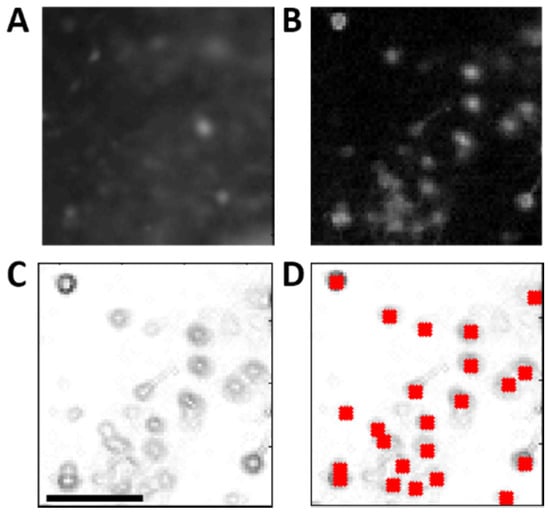
Figure 5.
Automated image processing for locating cell somata. (A) A raw single post-stimulus frame (512 × 512 pixels) is displayed from a series of frames (30 fps); (B) Image subtraction is performed to highlight the fluorescence difference post-stimulus from pre-stimulus; (C) The background is subtracted, and a gradient of the difference image is used to highlight the somata boundaries; (D) A circular Hough filter is applied to the gradient image to locate neuronal somata. Grid of 16 × 16 pixels (shown with red squares) mark the soma centers. Scale bar: 100 μm.
2.6. The Sigmoid Activation Model
A saturating nonlinearity, as was used in [], was chosen to fit to the neuronal probability of firing an action potential in response to a varying stimulus strength or duration. Specifically, a two-parameter sigmoid (Equation (1)) was used to describe this 1-D activation curve for cathodic square-pulse stimuli.
The sigmoid model provides an approximation for the stimulus needed to activate a particular neuron with any given probability. The input activation parameter, x, is either the stimulus current or pulse width, and the output is the probability, p, of a neuron to fire an action potential. The two parameters describing the sigmoid are b1, the midpoint of the sigmoid, which is the activation threshold and b2, the slope of the curve at the midpoint, which is the gain. Because the sigmoid describes a probability of activation, it spans from zero to one.
2.7. The Closed-Loop Search Algorithm
The closed-loop search procedure was divided into two halves: First, the collected stimulus-response data set was fit to the sigmoid model, and second, the sigmoid model was used to calculate the next stimulus to be delivered. The algorithm always first began with five open-loop stimuli that divided the stimulation space evenly before any curve fitting was performed. After the fifth iteration, the sigmoid model was analytically linearized, and a linear least-squares fit of the midpoint and slope parameters was performed to calculate a reasonable guess for the two sigmoid parameters—the sigmoid midpoint and the slope of the curve at the midpoint. All measured stimulus-evoked responses were equally weighted as zeros and ones. The output of the linear regression was used as an initial guess for a nonlinear least squares curve fit using the MATLAB Optimization Toolbox, which generated the best-fit sigmoid parameters. At this point, the sigmoid model has been fit to the dataset. The next stimulus value was then chosen in order to gain information about the sigmoid model midpoint and slope. To do this, the algorithm was designed to deliver the next stimulus along the slope of the sigmoid curve. A target neuronal activation probability goal was randomly chosen from the set of 0.25, 0.50 and 0.75, which spans the linear transition region of the sigmoid. The stimulus that was predicted to produce the firing probability goal was calculated using the sigmoid fit parameters and the activation probability goal. When a neuronal activation sigmoid had a nearly infinite slope, which was often the case when the dataset was still small early on in the experiment, the next stimulus chosen would be the same as the previously delivered stimulus. To ensure that the algorithm did not get stuck at one stimulus value, a random jitter was added to the stimulus up to 20% in either direction so that more data would be collected over the full range of the transition region of the activation curve. After every stimulus iteration, the linear and nonlinear curve-fits were run to update the model. The search algorithm is presented below in pseudo-code form.
- Collect data for five distinct stimulus levels.
- Fit the sigmoid model to all available data points (zeros and ones).
- Fit the linearly transformed sigmoid model to all zeros and ones in the dataset
- Use the linearly transformed sigmoid model, which derives from Equation (1), to solve for the fit parameters b1 and b2.x = −ln[(1/p − 1)/b2] + b1
- Use the linear fit parameters as an initial guess for a nonlinear curve fit of the model in Equation (1)
- Minimize the sum-squared error
- Use lsqcurvefit Matlab algorithm to calculate b1 and b2
- Select the stimulus parameter for the next step
- Select from the set of probabilities {0.25, 0.50, 0.75} using randperm Matlab function
- Calculate from the sigmoid model the corresponding stimulus value
- Solve the linearly transformed sigmoid model described above, which derives from Equation (1), for x—the next stimulus value.
- If stimulus value is same as previous step, add jitter up to 20% in stimulus value, according to a uniform random distribution.
- Apply the calculated stimulus value in the experiment
- Use calcium imaging and image processing determine if the stimulus-evoked change in measured fluorescence surpassed threshold.
- If convergence is not reached or if stimulus step count is not met, return to Step 2, else stop.
2.8. The Strength-Duration Activation Model
Neuronal activation in the 2-D strength-duration waveform space was modeled based on [] (Equation (2)).
The stimulus pulse width, PW, is the input; the stimulus current, I, is the output. The two model parameters are the rheobase, r, and the chronaxie, c. The rheobase describes the stimulus current below which a stimulus with infinite pulse width will not evoke an action potential, and the chronaxie describes the stimulus pulse width that corresponds to a stimulus current of twice the rheobase.
Once several sigmoids are constructed for a stimulus of e.g., strength, at multiple durations, a strength-duration model can be fit for a specific probability level by minimizing the sum squared error between the sigmoid-predicted probabilities at each duration, and the strength-duration model predicted probability.
2.9. Experimental Plan
The CL system for experimental examination of directly-evoked neuronal activity in response to a stimulus was used in four independent experiments. In the first experiment, an OL paradigm was used to explore the vast strength-duration waveform space. In the second experiment, the CL system was itself analyzed to assess convergence of the algorithm on the sigmoid model parameters used to describe a one-parameter activation curve. In the third experiment, the CL experimental system was used to investigate the strength-duration neuronal activation model with greater resolution in the stimulus waveform space. Finally, in the last experiment, the CL system was directly compared to an OL investigation.
3. Results
The automated system for optically measuring stimulus-evoked neuronal activation was used to characterize the response to a single extracellular stimulus pulse. In the 1-D stimulus pulse parameter space, neurons activate in a probabilistic manner that is well described by the sigmoid activation model (Equation (1)). We show that our closed-loop (CL) approach is effective and efficient at constructing the activation model. When compared to open-loop (OL) stimulation techniques, the CL approach quickly converges on the activation curve. The faster convergence rate of the CL approach is particularly important as the dimensionality of the parameter space increases. We analyze two particular stimulus parameters: the current (strength) and the pulse width (duration).
3.1. Open-Loop Characterization of the Strength-Duration Waveform Space
The stimulus-evoked neuronal response is a stochastic process. It can be defined by the probability of a given neuron firing with an action potential in response to an input stimulus. We characterized the stimulus-evoked activation of a single neuron using open-loop methodologies, using a sigmoidal activation model (Equation (1)) to define the probability of the neuron to fire an action potential when one of the stimulation parameters (strength or duration) is varied (Figure 6A). A randomized set of 1140 stimuli were delivered to the MEA spanning currents from 2 μA to 20 μA in 1 μA increments and pulse widths from 300 μs to 800 μs in 100 μs increments. One pulse was presented per stimulus iteration, and ten repetitions of each pulse were delivered in the experiment. Action potentials were extracted after each stimulus iteration using our fluorescence thresholding routine. We calculated stimulus-evoked neuronal response probabilities for the neuron of interest by averaging the ten responses delivered at each stimulus point. It was unknown, a priori, where the neuron’s activation curve would lie within the pulse parameter space. The activation curve generated from the 700 μs stimulus pulses spans the full range of stimulus currents from 2 μA to 20 μA (Figure 6A). The best-fit midpoint and slope parameters were 9.3 μA and 1.1, and the 0.25 to 0.75 probability range spans 2.0 μA. The sigmoid model, which was fit to the 700 μs data, was used to extract the predicted stimulus currents that would produce probability estimates ranging from 0.1 to 0.9 in steps of 0.2 (highlighted with a box, Figure 6B). Similar to the 700 μs data analysis, we generated 1-D sigmoidal curves for each of the other stimulus pulse widths (300, 400, 500, 600, and 800 μs).
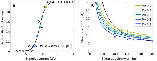
Figure 6.
Strength–duration curve fitting from neuronal activation data. A randomized set of 1140 stimuli were delivered to the MEA spanning 2–20 μA in 1 μA increments and pulse widths spanning 300–800 μs in 100 μs increments. Each stimulus was randomly repeated ten times to measure the activation probability with 0.1 resolution. (A) Average responses for each stimulus current with a 700 μs pulse width are plotted with open circles. Below 6 μA, no action potentials were detected, and above 11 μA action potentials were detected 10 out of 10 times. A non-linear least squares curve-fit of the sigmoid in Equation 1 was performed on the 700 μs data. The best fit is shown by the solid line. The sigmoid model was used to predict the stimuli that would produce activation probabilities ranging from 0.1 to 0.9 in 0.2 steps (closed circles, increasing probability from dark to light); (B) Model-predicted stimuli from (A), corresponding to activation probabilities ranging from 0.1 to 0.9, were plotted with solid circles and are outlined with a box. In the same manner as (A), sigmoid models were built for each of the sets of stimulus pulse-width data spanning 300–800 μs. These models were again used to predict a set of stimulus currents for the range of probability levels (vertical sets of solid circles). Strength-duration curves (solid lines) for each of the probability levels were created from a non-linear least squares curve-fit to the predicted points from the model in Equation (2). The shade of each curve corresponds to the equivalent probability level in (A). Probability steps of 0.2 were chosen for clarity. A constant-charge curve (6 nC) is shown as a reference (dotted line).
We generated a set of strength–duration probability isoclines in the 2-D stimulus-pulse parameter space from the 1-D sigmoids. These SD curves describe the probabilistic neuronal activation across this input parameter space (Figure 6B). As was described above, each sigmoid model was used to predict stimulus currents that would produce probability estimates from 0.1 to 0.9. These sets comprise a range of stimulus currents for each pulse width. A separate SD curve was calculated for each probability level by fitting Equation (2) to each set of model-predicted stimulus currents. It was necessary to use the model-predicted currents from the sigmoidal fits because it was unlikely that probability estimates were available at all probability levels of interest. The chronaxie and rheobase parameters for the 0.5 probability level were 535 μs and 5.2 μA.
3.2. Closed-Loop Analysis of Neuronal 1-D Activation Curves
We utilized the closed-loop routine to rapidly extract activation curves for a neuron in the search space of both the stimulus current and stimulus pulse width (Figure 7). We performed two sets of experiments, closing the loop around a single neuron, in which we held one of the stimulus parameters constant and varied the other parameter. The best-fit sigmoid (Equation (1)), defined for probabilities spanning from zero to one, was constructed for each of the stimulus current and pulse-width searches (Figure 7A,B). We calculated the averaged responses to each of the stimulus points. The 0.25 to 0.75 probability ranges span 2.2 μA (12.3–14.5 μA) for the constant-pulse-width search (fixed at 1000 μs), and 66 μs (366–432 μs), for the constant-current search (fixed at 30 μA). We calculated the best fit of each of the two sigmoid parameters, midpoint and slope, from the nonlinear least squares curve fit, after each stimulus iteration (Figure 7E–H). The shaded region marks the 95% confidence interval on those parameter fits. After the last iteration, the sigmoid midpoint and slope for the constant pulse-width search were 13.4 μA and 1.0 μA−1, and for the constant current search the parameter values were 399 μs and 0.03 μs−1. The convergence of the sigmoid midpoint and slope had three phases. In the first 20 stimulus iterations, the slopes are nearly infinite because stimulus repetitions were not likely to be present until the algorithm had converged on the sigmoid midpoint. In this phase, the midpoint is fluctuating and the slope is infinite. For the next 20 stimulus iterations, the midpoints are relatively constant, and as the search routine selected the stimulus values predicted to produce firing probabilities of 0.25, 0.50 and 0.75, repetitions began to emerge. After 40 stimulus iterations, the algorithm has produced a good estimate of the sigmoid midpoint and slope, and time is spent refining those parameters. It is important to note that even after 100 stimulus iterations, the confidence interval, while stable, does not converge to zero. It will always be non-zero because the data comprise a binomial set, in which the least squares fitting algorithm will always fit zeroes and ones to a smooth probability curve. The experimental measurements taken along the slope of the curve will therefore never overlay the actual curve, causing the confidence interval to remain non-zero [].
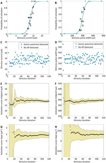
Figure 7.
Convergence of the closed-loop algorithm on the sigmoid model parameters. During an experiment, one stimulus parameter (current or pulse width) is fixed while the other is allowed to vary according to the closed-loop algorithm in order to find the neuronal activation curve. In one set of CL stimuli the pulse width was fixed at 1000 μs and the current was varied (A,C,E,G), and in another set of stimuli the current was fixed at 30 μA and the pulse width was varied (B,D,F,H); (A,B) The best-fit sigmoid from Equation (1) is plotted after the final stimulus iteration for each of the stimulus current and pulse-width searches. The activation curve is defined for probabilities spanning from zero to one. The averaged response to each of the stimulus values is depicted with open circles, which are proportional in size to the number of stimuli that were delivered at that value. The 10% to 90% probability regions span 4.3 μA and 130 μs. (C,D) The individual measured response to each stimulus is plotted as a dot to denote that an action potential was detected or an “X” to denote that no action potential was detected. The stimuli span the range of probabilities from the sigmoid activation curve. Two points were excluded in both plots from the extremes of the stimulus range, for clarity at the region of interest. The excluded stimuli at maximum intensity produced an action potential, and those at minimum intensity did not. (E–H) The convergence of the sigmoid midpoint and slope is shown with stimulus iteration. The black circles record the best fit of each of the two sigmoid parameters, midpoint and slope, from the nonlinear least squares curve fit of Equation (1), after each stimulus iteration. The shaded region marks the 95% confidence interval on the fit parameters.
3.3. Derivation of Probabilistic Strength-Duration Curves
The automated routine performed searches that were 1-D slices through the 2-D strength-duration waveform space in order to derive probabilistic strength-duration curves (Figure 8) for a single neuron in culture. We constructed these curves using two search directions in which one stimulus pulse parameter, the current or pulse width, was fixed while the other was allowed to vary. Each search yielded a sigmoid response curve in the horizontal, constant current, search direction or the vertical, constant pulse width, search direction. For each new search, the fixed parameter was then incremented, and the resulting sigmoid shifted.
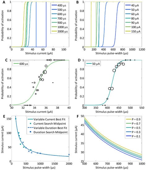
Figure 8.
Shifting sigmoids are used to generate the strength–duration curve. Closed-loop experiments were performed to generate two sets of sigmoid activation curves corresponding to various constant pulse width and constant current searches. (A,B) The pulse-width parameter was fixed in (A); and the current pulse parameter was fixed in (B); CL searches yielded sigmoid activation curves, which shifted to lower currents with increasing stimulus pulse width and shorter pulse widths with increasing stimulus pulse currents. The sigmoids appear to be extremely steep because the stimulus space is large; (C,D) Two sigmoid activation curves are highlighted by zooming in on the independent axis to demonstrate that the slopes span a significant stimulus range of 2.0 μA and 25 μs. The open circles overlaying the activation curves are a measure of the activation probability at a given stimulus level and are proportional in size to the number of stimuli that were applied at that stimulus; (E) The strength-duration curve, for a probability of 0.5, was built in two ways. Each of the sigmoid models were used to predict the stimulus that would produce an activation probability of 0.5 for the constant pulse-width (dots) and constant current (“X’s”) searches. The best fit of the strength-duration curve for both sets of searches (solid lines) was calculated using a nonlinear least squares curve fit of Equation (2); (F) Strength–duration curves were constructed using Equation (2) for probability levels spanning from 0.1 to 0.9 in 0.2 increments (increasing probability, from dark to light).
This produced two sets of shifting sigmoids where the activation threshold increased as the fixed parameter value decreased (Figure 8A,B). For the fixed-pulse-width searches ranging from 400 μs to 2000 μs, the sigmoids shift from 66.3 μA down to 23.0 μA, and for the fixed-current searches ranging from 40 μA to 150 μA, the sigmoids shift from 665 μs down to 140 μs. Although the curves appear to be nearly vertical, it is an artifact of the large stimulus range. When we zoom in on two of the sigmoids (Figure 8C,D), it becomes apparent that the slopes are finite. For the constant current search (Figure 8D), the midpoint and slope were 421 μs and 0.1 μs−1 and for the constant pulse-width search (Figure 8C), the midpoint and slope were 34.7 μA and 1.1 μA−1. The 0.25 to 0.75 probability ranges span 2.0 μA and 25 μs. Because the experiment was designed to estimate activation curves separately for fixed-current and fixed-duration stimulus pulses over very large stimulus parameter ranges, fewer data were collected along each slope, which resulted in a discrete measurements at various stimulus points that did not necessarily lie directly on the curve. The midpoints of each sigmoid (markers in Figure 8E), or 50% thresholds, were used as inputs into the SD non-linear curve-fitting routine using the model in Equation (2). These curves, which define the square pulse shapes that will produce a firing probability of 0.5 through SD space, were overlaid for the two data sets, and both search techniques produce similar output curves. The chronaxie and rheobase parameters for the constant current set of searches were 315 μs and 6.5 μA and were 360 μs and 5.9 μA for the constant pulse-width searches. The two sets of search data were combined, and the SD best-fit chronaxie and rheobase parameters were 316 μs and 6.5 μA for the 0.5 probability level. SD curves were calculated from the shifting sigmoids for the probability levels ranging from 0.1 to 0.9 in 0.2 steps (Figure 8F).
3.4. Comparison of Closed-Loop and Open-Loop Techniques
An experimental study was performed in order to compare closed-loop to open-loop stimulation methods (Figure 9) for another neuron in culture. A set of 250 stimuli were delivered using the CL approach and, subsequently, 250 stimuli were delivered using an OL approach. The OL stimuli were chosen in randomized order from a uniform distribution across the stimulus current space, and the pulse width was held constant. The stimulus current space spanned 0–40 μA with 0.2 μA steps. The OL study did not converge within the 250 trials, however, the CL study converged by the 100th stimulus iteration. The CL sigmoid slope was 2.8 μA−1 and the midpoint was 13.6 μA. Because the stimulator resolution was 0.2 μA, the maximum slope that could be estimated was about five. When the convergence of the fit parameters for the CL search was analyzed, we found that there were again three phases: In the first 20 stimulus iterations, the algorithm finds the sigmoid midpoint. It requires the next 80 iterations to find the slope. During these trials, the best-fit slope was near infinite (off of the chart in Figure 9E). In all subsequent stimulus iterations, the stimuli presented served to refine the fit parameters (Figure 9E). The best-fit sigmoid found after the final iteration (Figure 9A) has a probability range of 0.25 to 0.75 that spans 0.8 μA, and the stimulus values along the slope of the curve—13.0, 13.2, 13.4, 13.6, 13.8, and 14.0 μA—were measured 19, 27, 27, 35, 62, and 13 times, respectively. Whenever a stimulus to be delivered was equal in magnitude to the previous stimulus, a uniformly distributed jitter, up to 20% in either direction, was added to the stimulus. Because the sigmoid slope was steep, many of the stimuli that were delivered with jitter were beyond either knee of the curve and provided little additional information to the curve fit. Those stimuli can be seen in the clusters where the sigmoid curve saturates, either at probabilities of 0 or 1 (Figure 9A) and in the spread of the stimulus points in Figure 9C.
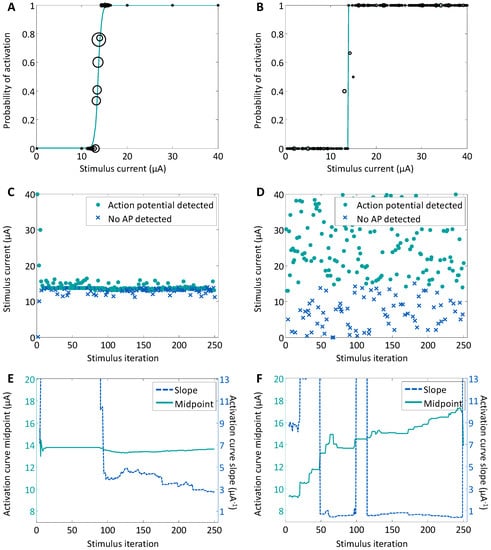
Figure 9.
Closed-loop versus open-loop experiments. Two sets of 250 stimuli were delivered to the culture via one electrode. In the closed-loop experiment, the model-based algorithm selected the stimuli in real-time (A,C,E); and in the open-loop experiment a random set of stimuli were chosen from the stimulus pulse parameter space (B,D,F); (A,B) The best fit of a sigmoid from Equation (1) is plotted after the 250th stimulus iteration. The averaged response to each of the stimulus currents is depicted with open circles, which are proportional in size to the number of stimuli that were delivered. (C,D) The individual measured response to each stimulus is plotted as a dot to denote that an action potential was detected or an “X” to denote that no action potential was detected. (E,F) The convergence of the sigmoid midpoint (solid line, left y-axis) and slope (dotted line, right y-axis) is shown with stimulus iteration. The sigmoid activation model was calculated in real-time after each stimulus iteration for the CL experiment and was calculated post-hoc for the OL experiment. The OL fit parameters did not converge.
In the OL experiment (Figure 9F), neither the sigmoid midpoint nor slope fit parameters converged within the 250 stimuli. While many other OL routines could have been employed, a uniform distribution of stimulus values throughout the stimulus parameter space was chosen because it is most general. Because most of the stimuli delivered were below the probability level of 0.1, or above 0.9, on the sigmoidal activation curve, they contributed little to improving the fit. This factor made the fit of the sigmoidal model highly sensitive to additional measurements lying within the 0.1–0.9 probability range. The model sensitivity is exemplified by the sudden drop in the midpoint parameter after the last stimulus and the multiple times that the slope parameter flips from under one to near infinite. The midpoint and slope were 16.9 μA and 0.4 μA−1 after iteration 249 and jumped to 13.9 μA and 114 μA−1 after the final iteration (Figure 9F).
4. Discussion
The application of closed-loop techniques offers significant potential to improve the efficacy of electrical stimulation in the characterization of stimulus-evoked neuronal responses []. Even a two-dimensional stimulus space—such as the aspect ratio of the stimulation pulse—can be sufficiently large to require optimized search approaches for characterization. Open-loop characterizations (parameter sweeps) are inefficient because of the probabilistic and sigmoidal natures of the neuronal activation functions. Because the activation is probabilistic, open-loop characterization requires multiple repetitions at a particular set of stimulus parameters to accurately measure that probability at that point in the parameter space. There is an inherent trade-off between probability resolution and stimulus resolution: Repeated measurements at each stimulus point increase probability resolution, at the expense of limiting the number of stimulus points that may be measured. The sigmoidal form of the activation function limits the useful range of stimulus parameters. Stimulating well below and above the knees of the sigmoidal activation curve provides no useful information given that the values in these regions are equal to 0 and 1, respectively. To best explore the stimulus parameter space, it is essential that experiment time is spent primarily in the stimulus regions that lie within the transition region, so that each additional measurement contributes significantly to improve the activation model. For example, Wallach et al. [] demonstrated that a neuronal response probability could be clamped over a long period of time using online feedback of the measured stimulus-evoked activity. Their approach emphasizes the strength of using a closed-loop system to evaluate any input-output relationship in neuronal systems. Closed-loop approaches are especially valuable for in vitro experimental model systems to capitalize on the advantage of a simplified preparation for higher throughput experimentation. For example, Newman et al. [] demonstrated applications ranging from neuronal population firing rate clamping to controlling network firing rates during epileptic events. Our closed-loop search routine, as shown in Figure 7, illustrates a powerful technique for rapidly characterizing neuronal activation by extensively probing the transition region of the sigmoid curve. Using our in vitro system, we were able to measure, with high confidence, the individual response of a specific neuron to electrical stimuli. Numerous approaches to scientific investigation benefit from the application of CL approaches to experimentation [], and our experimental system is designed to build on these achievements to further the development of high-throughput technologies.
4.1. Method Convergence
We evaluated the convergence of the sigmoidal fit parameters to determine the number of iterations at which the CL search routine could have exited. (In order to study this convergence, we delivered many more stimuli than were needed for optimal model parameterization.) In our experiments, the search routine only required approximately 20 stimulus iterations to converge on a relatively accurate measure of the activation threshold. Additional stimuli are required to determine an accurate estimate of the slope at the midpoint of sigmoidal transition region. For a relatively shallow slope, such as a slope of less than 1 μA−1 (Figure 7G), an additional 20 stimulus iterations were sufficient to estimate the slope accurately. For a steep slope, such as the slope of 3 μA−1 in Figure 9, 100 stimuli were required to estimate the slope accurately. We would argue that, for efficacy of stimulation, the difference between a slope of 3 μA−1 and infinity is negligible. If we make that assumption, an additional 20 stimulus iterations (after the midpoint convergence) were sufficient to determine that the slope was effectively infinite.
In the CL/OL study (Figure 9), the stimulus current range comprised 200 stimulus points (40 μA × 5 stimulus steps/μA). In a randomized OL study, this one-parameter sweep would require ~2000 stimuli to have ten repetitions at each stimulus value (200 stimulus points × 10 repetitions/stimulus point), or ~4000 stimuli to provide 20 repetitions at each stimulus value. In other words, the OL approach requires at least an order of magnitude more stimuli than the CL approach to develop the same level of confidence of the measured stimulus-evoked probability response.
Furthermore, the CL algorithm benefitted from the addition of adaptive jitter to the stimulus, depending on the estimate of the slope at the sigmoid midpoint. When the sigmoid slope was steep, the uniform distribution of jitter up to 20% in either direction produced stimuli that often fell beyond the transition region of the activation curve. These stimuli, therefore, were less useful than if they had been limited to a smaller range, such as a 5% jitter, around the sigmoid midpoint.
4.2. Limitations in the Presented Approach
We utilized an in vitro model neuronal system to specifically study only the direct activation of neurons. While other systems, including in vivo neuronal structures, may not have the simplicity of a synaptically silenced system like that which is presented here, we are interested in studying the way in which stimulus waveforms directly evoke activity in a given neuron. By eliminating down-stream synaptic communication in the model culture, we have essentially made a black box of the network. This then allows us to assume, for example, that in a scenario where neuronal communication is intact downstream, the expressed purpose of delivering stimuli through an array of micro-electrodes in only to activate an initial target neuron in a culture. In this study, the neurons were uncoupled from the surrounding network using synaptic blockers. While the CL system can estimate a neuronal activation threshold, the algorithm will require modification for application to tracking potentially non-stationary activation curves in a coupled network. In the studies presented herein, neuronal activation curves proved to be stable over the experiment, however, a particular neuron’s activation curve may not be stationary in the presence of synaptic network input.
There are limitations in the CL approach when it is applied to many neurons in the same experiment. The experiments conducted in this study were focused on a single neuron. While the system simultaneously collected activation data for all neurons within the imaging area, the CL optimized search routine was focused on one specific neuron. Therefore, the activation data collected for other neurons within the imaging area were not assured to lie in their sigmoidal transition regions. The OL approach has an advantage for measuring the activation of a large population of neurons within an experiment. Although the resolution along the slope of all curves will be low, neuronal activation curves for all measured neurons can be estimated simultaneously.
While the calcium-sensitive dye Fluo-5F was specifically chosen in this study for its high signal-to-noise ratio (SNR) and its low binding affinity (as to not hinder normal cell function), it has a slower response than dyes of other classes, such as voltage-sensitive dyes (VSDs). The use of Fluo-5F for this study is ideal, as neurons are synaptically blocked and only the evoked response is considered. For future studies where more physiologically relevant conditions are studied, it may be necessary to use high-speed video in conjunction with VSDs to image neuronal activity. The use of higher temporal-responsivity VSDs, to distinguish between events with fast subcomponents such as a burst of multiple action potentials, demands a video frame rate of at least a couple of hundred frames per second. A significantly faster frame rate carries with it an inherent reduction in the SNR of the dye signal due to the reduced time over which the measured signal is averaged, however, the continual improvements expected both in camera technology and molecular probes shall improve the overall efficacy of VSD indicators.
Optical imaging also limits the experimental approach. Irreversible photobleaching of the indicator fluorophore, which occurs with each light exposure, ultimately limits the number of stimulus trials that can be delivered during an experiment. The limited experimental time underscores the need to efficiently characterize the system. Additionally, there are limitations in the direct applicability to in vivo studies and clinical applications. Optical imaging is technically demanding in vivo, and many factors limit the ability to successfully implement such techniques in clinical applications. Both the tendency of light to scatter and the presence of native chromophores result in an effective limit to the depth that can be imaged in vivo, which significantly limits neuronal accessibility for imaging. It is possible to replace optical recording with electrical recording, but improvements would need to be made in spike sorting to causally match electrically recorded signals to the optical ground truth that is available using in vitro optical methods.
4.3. Improving Stimulus Selectivity and Waveform Shaping
Future approaches that incorporate optimized search strategies can improve the inefficiency of neuronal characterization applied to a large population of neurons. Different search directions can potentially be used for different regions of the SD parameter space because the activation of a neuron is sigmoidal for both vertical and horizontal slices through the space. For example, in Figure 8E, a 10 μA constant current, horizontal search would not have converged because 10 μA falls below the asymptotic rheobase of the curve. Instead, a constant pulse-width, vertical search will converge for long pulse widths. Conversely, a constant current search should be used for the high-current, short-pulse-width parameter region. For these reasons, the constant pulse-width searches are better fit to the right-hand portion of the strength-duration curve and the constant current searches are better fit to the left-hand portion of the curve. When mapping multiple neuronal activation curves in a single experiment, it may become more efficient to expand the search strategy to include many directions within the SD space (e.g., diagonally, at 45°). The activation models can help to inform these decisions in real time.
Future stimulation experiments can use this modular system to deliver stimuli of many different waveforms, including biphasic current pulses, voltage-controlled pulses, or less-discretized so-called noisy waveforms. High-throughput experimentation will also enable the direct comparison of SD parameters, including both the chronaxie and rheobase, across stimulus shapes and electrode types. The probabilistic nature of stimulus-evoked neuronal activation can be exploited to improve the selectivity of stimulation techniques. For example, two square pulses delivering the same charge, but with different aspect ratios, activate a neuron with differing probabilities. The product of the stimulus strength and duration is the charge delivered at the electrode, but the charge alone is insufficient to predict activation. The shape of the strength-duration curve does not follow a constant-charge curve in part because of the asymptotic feature, the rheobase. As an example, a constant charge curve is plotted in Figure 6B. Two square pulses of equal charge lie along this 6 nC line, one of 400 μs pulse width (15 μA) and one with 800 μs pulse width (7.5 μA). The 400 μs pulse has a high activation probability of 0.91, while the 800 μs pulse is only 0.17. This demonstrates that stimuli of the same total charge can activate a neuron with very different probabilities.
5. Conclusions
We used a model system to demonstrate our approach to showing that closed-loop electrical stimulation converges to a stimulus activation model in significantly fewer iterations than do open-loop techniques, while resulting in a higher-resolution model. Both the convergence rate and the model accuracy are requirements for measuring and controlling neuronal activation across a large parameter space. Our CL routine quickly identified the relevant activation-curve features so that they could be more thoroughly probed to increase our measurement confidence. We demonstrated that the stimulus-evoked neuronal response is probabilistic, and by using our CL imaging system and micro-stimulation technology, we were able to stimulate a neuron with various probabilities. By exploiting the shape of the strength-duration curve we could activate a neuron with different probabilities by varying the aspect ratio of a constant-charge stimulus pulse. We demonstrated the advantages of utilizing in vitro dissociated cortical neuronal cultures to study neuronal activation. This reduced biological preparation provided us both with an optical ground truth for measuring evoked neuronal activity and with fine-grained electrical access to individual neurons. In addition, our experimental system inherently enables long-duration experiments, which can be readily replicated in a high-throughput manner. All types of in vitro experimentation, which make use of these advantages, are becoming more and more important for developing new technologies and methods. Exploring complex parameter spaces around these evoked responses is the challenge, and an in vitro preparation readily provides access to measurements that may otherwise be unattainable.
Furthering the understanding of the way in which electrical stimuli directly affect neuronal activity is necessary in order to design stimuli that better activate neurons and neuronal populations. Closed-loop strategies are indispensable for developing techniques to precisely activate neurons, which is critical for the advancement of both in vitro and in vivo studies.
Acknowledgments
This work was partially funded by the National Institutes of Health (NIH) through grant EB006179 and NIH-NINDS 1R01NS079757 and was partially funded by the National Science Foundation (NSF) through the NSF-COPN grant 1238097, NSF-GRFP DGE-0802270 and NSF-IGERT DGE-0333411. It was also partially funded by Khalifa University of Science, Technology and Research (KU).
Author Contributions
M.L.K., M.A.G., S.M.P. and S.P.D. conceived and designed the experiments; M.L.K. and G.S.G. wrote the software for interfacing with hardware and performed the experiments; M.L.K., M.A.G., and S.P.D analyzed the data; S.M.P. and S.P.D. contributed reagents/materials; M.L.K. wrote the paper.
Conflicts of Interest
The authors declare no conflict of interest.
References
- Fritsch, G.; Hitzig, E. Electric excitability of the cerebrum (Über die elektrische Erregbarkeit des Grosshirns). Epilepsy Behav. 2009, 15, 123–130. [Google Scholar] [CrossRef] [PubMed]
- Cohen, M.R.; Newsome, W.T. What electrical microstimulation has revealed about the neural basis of cognition. Curr. Opin. Neurobiol. 2004, 14, 169–177. [Google Scholar] [CrossRef] [PubMed]
- Clark, K.L.; Armstrong, K.M.; Moore, T. Probing neural circuitry and function with electrical microstimulation. Proc. R. Soc. B Biol. Sci. 2011, 278, 1121–1130. [Google Scholar] [CrossRef] [PubMed]
- Borchers, S.; Himmelbach, M.; Logothetis, N.; Karnath, H.O. Direct electrical stimulation of human cortex—The gold standard for mapping brain functions? Nat. Rev. Neurosci. 2011, 13, 63–70. [Google Scholar] [CrossRef] [PubMed]
- Mandonnet, E.; Winkler, P.; Duffau, H. Direct electrical stimulation as an input gate into brain functional networks: Principles, advantages and limitations. Acta Neurochir. 2010, 152, 185–193. [Google Scholar] [CrossRef] [PubMed]
- Dulay, M.F.; Murphey, D.K.; Sun, P.; David, Y.B.; Maunsell, J.H.; Beauchamp, M.S.; Yoshor, D. Computer-controlled electrical stimulation for quantitative mapping of human cortical function: Technical note. J. Neurosurg. 2009, 110, 1300–1303. [Google Scholar] [CrossRef] [PubMed]
- Wallach, A.; Eytan, D.; Gal, A.; Zrenner, C.; Marom, S. Neuronal response clamp. Front. Neuroeng. 2011, 4, 3. [Google Scholar] [CrossRef] [PubMed]
- Keren, H.; Marom, S. Controlling neural network responsiveness: Tradeoffs and constraints. Front. Neuroeng. 2014, 7, 11. [Google Scholar] [CrossRef] [PubMed]
- Weiss, G. Sur la possibilite de rendre comparables entre eux les appareils servant a l’excitation electrique. Arch. Ital. Biol. 1901, 35, 413–446. [Google Scholar]
- Lapicque, L. Quantitative investigations of electrical nerve excitation treated as polarization. 1907. Biol. Cybern. 2007, 97, 341–349. [Google Scholar] [PubMed]
- Gustafsson, B.; Jankowska, E. Direct and indirect activation of nerve cells by electrical pulses applied extracellularly. J. Physiol. 1976, 258, 33–61. [Google Scholar] [CrossRef] [PubMed]
- Holsheimer, J.; Dijkstra, E.A.; Demeulemeester, H.; Nuttin, B. Chronaxie calculated from current-duration and voltage-duration data. J. Neurosci. Methods 2000, 97, 45–50. [Google Scholar] [CrossRef]
- Mogyoros, I.; Kiernan, M.C.; Burke, D. Strength-duration properties of human peripheral nerve. Brain J. Neurol. 1996, 119 Pt 2, 439–447. [Google Scholar] [CrossRef]
- Rattay, F.; Paredes, L.P.; Leao, R.N. Strength-duration relationship for intra-versus extracellular stimulation with microelectrodes. Neuroscience 2012, 214, 1–13. [Google Scholar] [CrossRef] [PubMed]
- Nowak, L.G.; Bullier, J. Axons, but not cell bodies, are activated by electrical stimulation in cortical gray matter. Exp. Brain Res. 1998, 118, 477–488. [Google Scholar] [CrossRef] [PubMed]
- Lee, S.W.; Eddington, D.K.; Fried, S.I. Responses to pulsatile subretinal electric stimulation: Effects of amplitude and duration. J. Neurophysiol. 2013, 109, 1954–1968. [Google Scholar] [CrossRef] [PubMed]
- Mahmud, M.; Vassanelli, S. Differential Modulation of Excitatory and Inhibitory Neurons during Periodic Stimulation. Front. Neurosci. 2016, 10. [Google Scholar] [CrossRef] [PubMed]
- Arsiero, M.; Luscher, H.-R.; Giugliano, M. Real-time closed-loop electrophysiology: Towards new frontiers in in vitro investigations in the neurosciences. Arch. Ital. Biol. 2007, 145, 193–209. [Google Scholar] [PubMed]
- Benda, J.; Gollisch, T.; Machens, C.K.; Herz, A.V. From response to stimulus: Adaptive sampling in sensory physiology. Curr. Opin. Neurobiol. 2007, 17, 430–436. [Google Scholar] [CrossRef] [PubMed]
- Zrenner, C.; Eytan, D.; Wallach, A.; Thier, P.; Marom, S. A generic framework for real-time multi-channel neuronal signal analysis, telemetry control, and sub-millisecond latency feedback generation. Front. Neurosci. 2010, 4, 173. [Google Scholar] [CrossRef] [PubMed]
- DiMattina, C.; Zhang, K. Active data collection for efficient estimation and comparison of nonlinear neural models. Neural Comput. 2011, 23, 2242–2288. [Google Scholar] [CrossRef] [PubMed]
- Newman, J.P.; Zeller-Townson, R.; Fong, M.F.; Desai, S.A.; Gross, R.E.; Potter, S.M. Closed-loop, multichannel experimentation using the open-source NeuroRighter electrophysiology platform. Front. Neural Circuits 2012, 6, 98. [Google Scholar] [CrossRef] [PubMed]
- Vassanelli, S.; Mahmud, M.; Girardi, S.; Maschietto, M. On the way to large-scale and high-resolution brain-chip interfacing. Cogn. Comput. 2012, 4, 71–81. [Google Scholar] [CrossRef]
- Krook-Magnuson, E.; Gelinas, J.N.; Soltesz, I.; Buzsáki, G. Neuroelectronics and Biooptics: Closed-Loop Technologies in Neurological Disorders. JAMA Neurol. 2015, 72, 823–829. [Google Scholar] [CrossRef] [PubMed]
- Rosin, B.; Slovik, M.; Mitelman, R.; Rivlin-Etzion, M.; Haber, S.N.; Israel, Z.; Vaadia, E.; Bergman, H. Closed-loop deep brain stimulation is superior in ameliorating parkinsonism. Neuron 2011, 72, 370–384. [Google Scholar] [CrossRef] [PubMed]
- Schiller, Y.; Bankirer, Y. Cellular mechanisms underlying antiepileptic effects of low-and high-frequency electrical stimulation in acute epilepsy in neocortical brain slices in vitro. J. Neurophysiol. 2007, 97, 1887–1902. [Google Scholar] [CrossRef] [PubMed]
- Weihberger, O.; Okujeni, S.; Mikkonen, J.E.; Egert, U. Quantitative examination of stimulus-response relations in cortical networks in vitro. J. Neurophysiol. 2013, 109, 1764–1774. [Google Scholar] [CrossRef] [PubMed]
- Smetters, D.; Majewska, A.; Yuste, R. Detecting action potentials in neuronal populations with calcium imaging. Methods 1999, 18, 215–221. [Google Scholar] [CrossRef] [PubMed]
- Edelstein, A.; Amodaj, N.; Hoover, K.; Vale, R.; Stuurman, N. Computer control of microscopes using μManager. Curr. Protoc. Mol. Biol. 2010, 14. [Google Scholar] [CrossRef]
- Potter, S.M.; DeMarse, T.B. A new approach to neural cell culture for long-term studies. J. Neurosci. Methods 2001, 110, 17–24. [Google Scholar] [CrossRef]
- Wagenaar, D.A.; Pine, J.; Potter, S.M. Effective parameters for stimulation of dissociated cultures using multi-electrode arrays. J. Neurosci. Methods 2004, 138, 27–37. [Google Scholar] [CrossRef] [PubMed]
- Bakkum, D.J.; Chao, Z.C.; Potter, S.M. Long-term activity-dependent plasticity of action potential propagation delay and amplitude in cortical networks. PLoS ONE 2008, 3, e2088. [Google Scholar] [CrossRef] [PubMed]
- Grewe, B.; Langer, D.; Kasper, H.; Kampa, B.; Helmchen, F. High-speed in vivo calcium imaging reveals neuronal network activity with near-millisecond precision. Nat. Methods 2010, 7, 399–405. [Google Scholar] [CrossRef] [PubMed]
- Ranganathan, G.; Koester, H. Optical Recording of Neuronal Spiking Activity From Unbiased Populations of Neurons With High Spike Detection Efficiency and High Temporal Precision. J. Neurophysiol. 2010, 104, 1812–1824. [Google Scholar] [CrossRef] [PubMed]
- Vogelstein, J.; Watson, B.; Packer, A.; Yuste, R.; Jedynak, B.; Paninski, L. Spike Inference from Calcium Imaging Using Sequential Monte Carlo Methods. Biophys. J. 2009, 97, 636–655. [Google Scholar] [CrossRef] [PubMed]
- Peng, T. Detect Circles with Various Radii in Grayscale Image via Hough Transform. 2005. Available online: http://www.mathworks.com/matlabcentral/fileexchange/9168 (accessed on 2 February 2012).
- Cox, D.R. The regression analysis of binary sequences. J. Royal Stat. Soc. Ser. B (Methodol.) 1958, 215–242. [Google Scholar]
- Kuykendal, M.L.; Potter, S.M.; Grover, M.A.; DeWeerth, S.P. Targeted Stimulation Using Differences in Activation Probability across the Strength–Duration Space. Processes 2017, 5, 14. [Google Scholar] [CrossRef]
© 2017 by the authors. Licensee MDPI, Basel, Switzerland. This article is an open access article distributed under the terms and conditions of the Creative Commons Attribution (CC BY) license (http://creativecommons.org/licenses/by/4.0/).