Model-Based Reactor Design in Free-Radical Polymerization with Simultaneous Long-Chain Branching and Scission

Abstract

Polymers are the products of processes and their microstructure can be changed significantly by the reactor systems employed, especially for nonlinear polymers. The Monte Carlo simulation technique, based on the random sampling technique, is used to explore the effect of reactor types on the branched polymer structure, formed through free-radical polymerization with simultaneous long-chain branching and scission, as in the case of low-density polyethylene synthesis. As a simplified model for a tower-type multi-zone reactor, a series of continuous stirred-tank reactors, consisting of one big tank and the same N-1 small tanks is considered theoretically. By simply changing the tank arrangement, various types of branched polymers, from star-like globular structure to a more randomly branched structure, can be obtained, while keeping the following properties of the final products, the monomer conversion to polymer, the average branching and scission densities, and the relationship between the mean-square radius of gyration and molecular weight.

1. Introduction

Nonlinear polymer formation under a kinetically controlled condition is, in general, history-dependent, and the history of every polymer molecule determines the properties of final product polymers. The molecular architecture can be very complex; however, the history-dependence opens up the opportunities to control the nonlinear structure through various types of reactor operation.

In this article, free-radical polymerization that involves chain transfer to polymer, leading to long-chain branching and scission, as in the case of high-pressure polymerization of ethylene to produce low-density polyethylene [1,2], is considered. As shown in Figure 1, the birth time of the chains, C₁ and C₂ must be some time after that of A or A’. There is a definite time order for the chain connection statistics.

Figure 1. Schematic representation of the process of chain transfer to polymer, leading to long-chain branching and scission.

Figure 1. Schematic representation of the process of chain transfer to polymer, leading to long-chain branching and scission.

When the scission reaction is involved together with long-chain branching, the time sequence of branching and scission must be properly accounted for. This kind of reaction system cannot be fully represented by a simple set of population balance differential equations [3,4,5,6,7]. On the other hand, by application of Monte Carlo (MC) method, based on the random sampling technique [8,9], history-dependence of branching and scission can be fully accounted for [7,10,11,12]. In this MC simulation method, the structure of each polymer molecule can be observed directly on the computer screen, and very detailed structural information can be obtained. On the basis of such detailed structural information, it is possible to determine the viscoelastic properties of branched polymers [13].

This simulation method can be used to investigate the effect of reactor type on the formed branched structure. Following the fundamentals of chemical reaction engineering [14], consider how the difference of an ideal plug flow reactor (PFR) and an ideal continuous stirred-tank reactor (CSTR) affects the present polymerization system. Note that a PFR is equivalent to a batch reactor, in which the length in a PFR can be converted to time in a batch reactor. Figure 2 shows the MC simulation results [12] of the weight fraction distribution for the polymers synthesized in a PFR and in a CSTR. In the simulation, the final average branching density ($\overline{\rho }=2.22\times {10}^{-3}$), as well as the final scission density ($\overline{\eta }=1.11\times {10}^{-4}$), is set to be the same for both types of reactors. The independent variable shown in the figure is the logarithm of degree of polymerization (DP), log₁₀P, as usually employed in the gel permeation chromatography (GPC) measurement. The high DP tail extends more significantly in a CSTR, and the weight-average DP is larger for the product in a CSTR, even though the average branching density level is set to be the same.

Figure 2. Weight fraction distribution of polymers formed in a PFR and in a CSTR, when the average branching density, as well as the average scission density, is set to be the same for both types of reactors [12]. The kinetic parameters used are the same as C1, shown later in Table 2 of this article.

Figure 2. Weight fraction distribution of polymers formed in a PFR and in a CSTR, when the average branching density, as well as the average scission density, is set to be the same for both types of reactors [12]. The kinetic parameters used are the same as C1, shown later in Table 2 of this article.

Figure 3 shows the MC simulation results [12] for the relationship between the branching density ρ and the degree of polymerization P. The branching density is defined as the fraction of units having a branch point. In Figure 3a,b, each dot represents ρ and P of each polymer molecule simulated, and the solid blue curve with circular symbols shows the average ρ within small ΔP intervals, which is the estimate of the average branching density of polymers having degree of polymerization P, $\overline{\rho }(P)$. The dashed black line shows the average branching density of the whole system, $\overline{\rho }$. The value of $\overline{\rho }(P)$ increases with P, but reaches a constant limiting value ${\rho }_{P\to \infty }$, and ${\rho }_{P\to \infty }$ is larger than the average branching density of the whole system, $\overline{\rho }$. This is a rather general characteristic of the branched polymer systems [9], including the hyperbranched polymers [15]. Figure 3c shows the comparison of $\overline{\rho }(P)$ for a PFR and for a CSTR. The limiting branching density is larger for the CSTR.

Figure 3. Relationship between branching density ρ and degree of polymerization P for the branched polymers formed in (a) a PFR and in (b) a CSTR, and (c) $\overline{\rho }(P)$ for both types of reactors. The calculation condition is the same as in Figure 2.

Figure 3. Relationship between branching density ρ and degree of polymerization P for the branched polymers formed in (a) a PFR and in (b) a CSTR, and (c) $\overline{\rho }(P)$ for both types of reactors. The calculation condition is the same as in Figure 2.

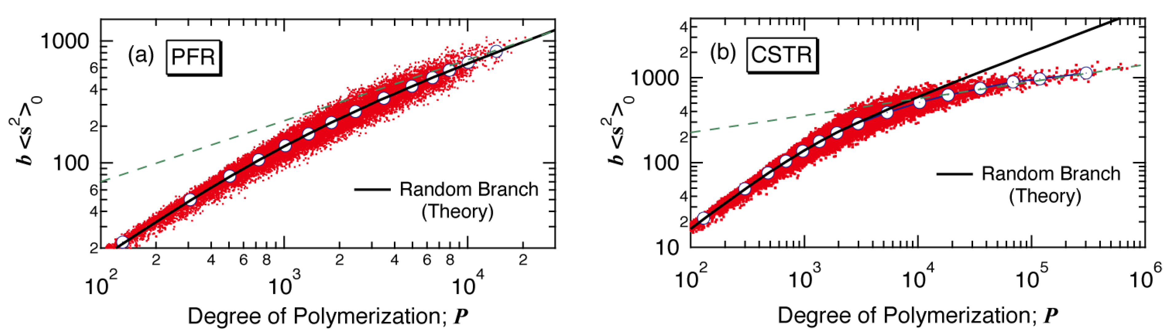
Figure 4 shows the relationship between the mean square radius of gyration for the unperturbed chains <s²>₀ and P. In the figure, b is a constant defined by b = u/l², where u is the number of monomeric units in a random walk segment, and l is the length of a random walk segment. Each dot in Figure 4 represents <s²>₀ and P-value of each polymer molecule simulated, and the circular symbols show the average values of <s²>₀ within small ΔP intervals, which are the estimates of the average <s²>₀ of polymers having DP, P. For randomly branched polymers, the radii of gyration is known to be given by the Zimm-Stockmayer equation [16], represented by:

$$b{\langle {\text{s}}^2\rangle }_{\text{0}}=\frac{P}{6}{\left[{\left(1+\frac{m_P}{7}\right)}^{0.5}+\frac{4m_P}{9\pi }\right]}^{-0.5}$$

(1)

where $m_P$ is the number of branch points with degree of polymerization P, and for the present case it can be estimated from:

$$m_P=P\overline{\rho }(P)$$

(2)

Figure 4. Relationship between the mean-square radius of gyration <s²>₀ and degree of polymerization P for the branched polymers formed in (a) a PFR and in (b) a CSTR [12]. In the figure, b is a constant defined by b = u/l², where u is the number of monomeric units in a random walk segment, and l is the length of a random walk segment. The black solid curve shows the relationship for random branched polymers. The slope of broken straight line (green) for (a) is 0.5, while that for (b) is 0.2.

Figure 4. Relationship between the mean-square radius of gyration <s²>₀ and degree of polymerization P for the branched polymers formed in (a) a PFR and in (b) a CSTR [12]. In the figure, b is a constant defined by b = u/l², where u is the number of monomeric units in a random walk segment, and l is the length of a random walk segment. The black solid curve shows the relationship for random branched polymers. The slope of broken straight line (green) for (a) is 0.5, while that for (b) is 0.2.

In Figure 4, the radii of gyration of randomly branched polymers having the branching density, $\overline{\rho }(P)$ is shown by a black curve. For a PFR, the radius of gyration is essentially the same as for the random branched polymers, as shown in Figure 4a. In a PFR or a batch reactor, <s²>₀ is close to that for the random branched polymers, at least for low conversion regions, while the <s²>₀-values tend to become slightly larger than those for the random branched polymers at higher conversions [17]. On the other hand, for a CSTR, the <s²>₀-values for large polymers are significantly smaller than the random branched polymers, as shown in Figure 4b.

Incidentally, because the $\overline{\rho }(P)$-value reaches a constant value at large P’s, the <s²>₀ curve for the random branched polymer, represented by Equation (1), follows the power law with <s²>₀ $\propto P^{0.5}$ for $P\to \infty$. In Figure 4a, the broken line shows the slope with 0.5. On the other hand, for a CSTR, it is not clear if the power law holds for large polymers, but the broken line drawn as a trial shows the slope with 0.2.

Table 1 summarizes the characteristics of PFR and CSTR for free-radical polymerization with chain transfer to polymer. Note that Table 1 applies for low scission frequency cases. Because the polymer transfer reaction is the reaction between a polymer and a polymer radical, larger polymer concentration promotes the chain transfer reaction. With a CSTR, the polymer concentration is high throughout the polymerization. If the final conversion is set to be the same for both types of reactors, the average branching density is larger for the polymers synthesized in a CSTR. In the present example, because the final average branching density is set to be the same, the final conversion must set to be larger for a PFR. It is interesting to note that the weight-average DP, ${\overline{P}}_{\text{w}}$ is larger for a CSTR, even though the average branching and scission densities are the same for both types of reactors. As shown in Figure 2, the molecular weight distribution of polymers formed in a CSTR is broader.

Table 1. Comparison of PFR and CSTR, under condition where the final average branching density is set to be the same for both types of reactors.

Property of product polymer	PFR (or Batch)	CSTR
Final conversion	>
Weight-average DP, ${\overline{P}}_{\text{w}}$	<
Branching density of large polymers, ${\rho }_{P\to \infty }$	<
<s2>0, compared with random branched polymers	Almost the same. (May become larger at higher conversions.)	Significantly smaller for large polymers.

Table 1. Comparison of PFR and CSTR, under condition where the final average branching density is set to be the same for both types of reactors.

Property of product polymer	PFR (or Batch)	CSTR
Final conversion	>
Weight-average DP, ${\overline{P}}_{\text{w}}$	<
Branching density of large polymers, ${\rho }_{P\to \infty }$	<
<s2>0, compared with random branched polymers	Almost the same. (May become larger at higher conversions.)	Significantly smaller for large polymers.

The branching density of large polymers, represented by ${\rho }_{P\to \infty }$ is larger for a CSTR, as shown in Figure 3. For the polymers synthesized in a PFR, the radius of gyration of polymers having the degree of polymerization P is essentially the same as that for the random branched polymers. It would be reasonable to consider that the branched structure formed in a PFR is close to randomly branched. On the other hand, as Figure 4b shows, the polymers formed in a CSTR possess much smaller radius of gyration compared with that for the random branched polymers with the same P-value.

As the textbook describes [14], when the multiple CSTRs are connected in series, the residence time distribution approaches to that of a PFR, as the number of tanks increases. The tanks-in-series model was applied to the present reaction system [18] to confirm that as the number of tanks increases the produced polymers approach to those formed in a PFR. Figure 5 shows how the relationship between <s²>₀ and P changes by increasing the total number of tanks.

The MC simulation method employed in refs. [7,12,18] can be used to investigate the effect of reaction environment change on the formed branched polymer structure, which may lead to a discovery of novel type of reactor systems. In this article, a series of continuous stirred-tank reactors, consisting of one big tank and the same N-1 small tanks is discussed by using the data reported in reference [7] and newly created MC simulation data. The possibility of model-based reactor design for the nonlinear polymerization system is explored.

Figure 5. Effect of the number of CSTRs in the tanks-in-series model on the relationship between the mean-square radius of gyration <s²>₀ and degree of polymerization P. The MC simulation data were taken from [18].

Figure 5. Effect of the number of CSTRs in the tanks-in-series model on the relationship between the mean-square radius of gyration <s²>₀ and degree of polymerization P. The MC simulation data were taken from [18].

2. Simulation Method

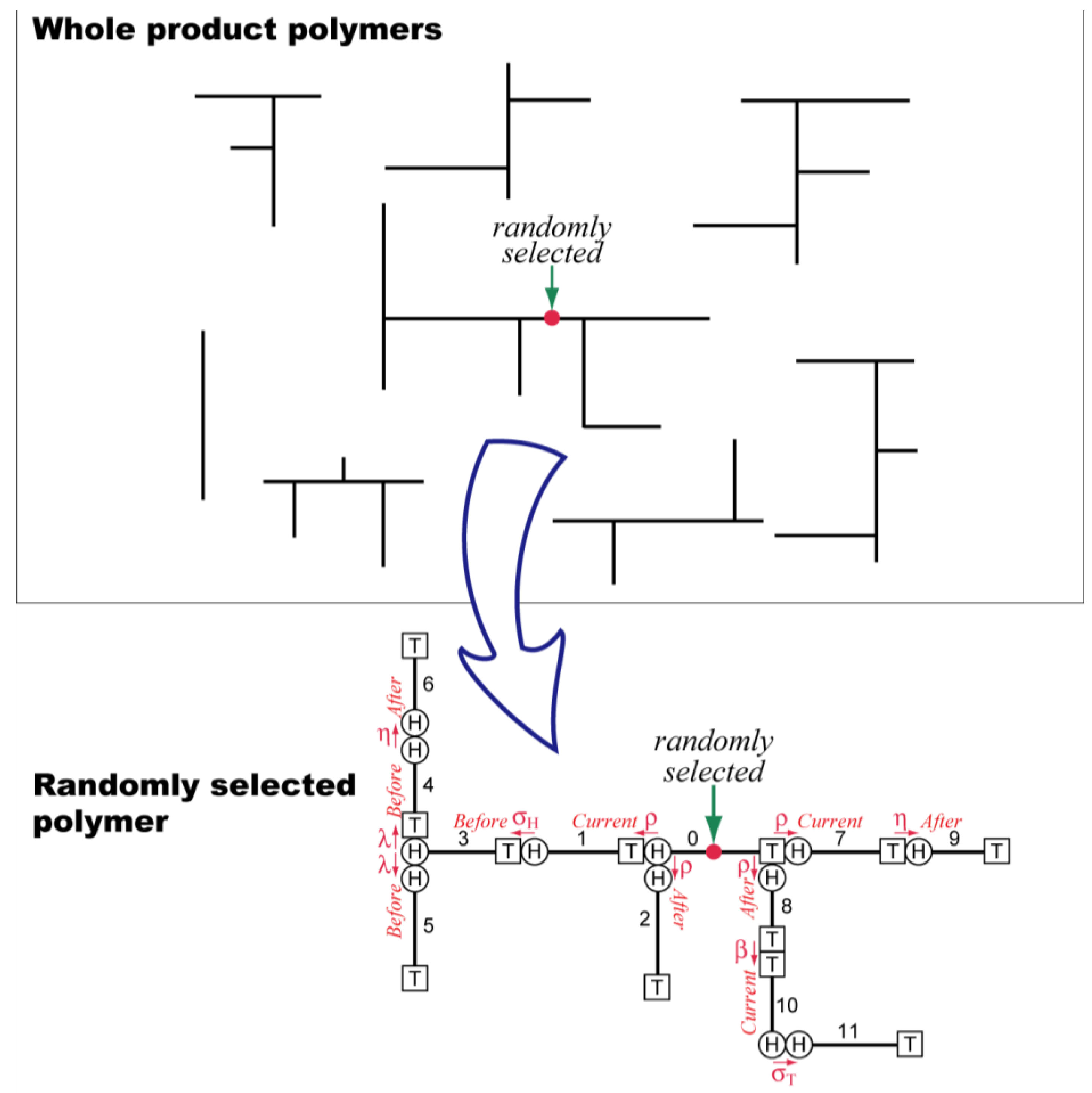
The random sampling technique [8,9] is used to estimate the properties of final product polymers. In this method, a polymer molecule is selected randomly from the product polymers, and the molecular structure is reconstructed by following the history of this particular polymer molecule, as schematically represented by Figure 6.

Figure 6. Schematic representation of the concept of random sampling technique.

Figure 6. Schematic representation of the concept of random sampling technique.

When the random sampling technique is applied to the Monte Carlo method, a large number of polymers are sampled, and the statistical properties of the whole system are determined effectively. In this method, the system size considered is infinitely large, and therefore, the system boundary problem does not occur. In addition, the amount of calculation required does not increase significantly by increasing the number of CSTRs in series. This MC simulation does not proceed in the order of reaction time, as in the most of other MC methods [19]. Looking from the given chain, the chains with different birth times are connected back and forth by following the reaction history that particular polymer molecule has experienced.

The selection of polymer molecules can be done both on the number and the weight basis [9]. In the case shown in Figure 6, a polymer molecule is chosen by selecting one monomeric unit randomly, which is the selection on the weight basis. For example, the weight-average degree of polymerization, ${\overline{P}}_{\text{w}}$ can be obtained by simply taking the arithmetic average of the sample. Incidentally, the analytic representation of ${\overline{P}}_{\text{w}}$ can always be obtained by using the random sampling technique [20,21,22,23,24].

The elementary reactions considered here are as follows. Initiation (rate represented by R_I), propagation (R_p), chain transfer to small molecules including monomer, solvent and chain transfer agents (R_f), bimolecular termination by disproportionation (R_td) and by combination (R_tc), and chain transfer to polymer (R_fp) leading to long-chain branching (R_b) and chain scission (R_s), with R_fp = R_b + R_s.

The backbiting reaction to form short-chain branching, typically consisting of several carbon atoms, is not considered explicitly, because it has negligible effects on the formed molecular weight distribution and the radii of gyration, which are the major topics of the present investigation. However, the hydrogen abstraction reaction is much more significant for the tertiary carbon atom, rather than the secondary carbon, and therefore, the polymer transfer reactions would be promoted by the backbiting reactions. Because the location of the tertiary carbon atoms along the chain could be considered random, the overall rate coefficients for the branching and the scission reactions k_b and k_s given below are employed [7,12,18].

$$R_{\text{b}}=k_{\text{b}}[{\text{R}}^{•}]Q_1$$

(3)

$$R_{\text{s}}=k_{\text{s}}[{\text{R}}^{•}]Q_1$$

(4)

where $[{\text{R}}^{•}]$ is the total radical concentration, and $Q_1$ is the first moment of the polymer distribution, representing the total number of monomeric units in polymer.

$$Q_1={\displaystyle \sum _{P=1}^{\infty }P[{\text{P}}_P]}$$

(5)

where $[{\text{P}}_P]$ is the concentration of polymer having degree of polymerization, P.

In a strict sense, the long-chain branching reaction shown in Figure 1 is a second order reaction between an internal radical and a monomer, while the scission reaction is the first order reaction of the internal radical, and relative contribution would change during polymerization. However, it was found earlier that such kinetic differences could be neglected [25] for the cases with the final conversion smaller than ca. 0.25, which is normally satisfied for the commercial low-density polyethylene production processes.

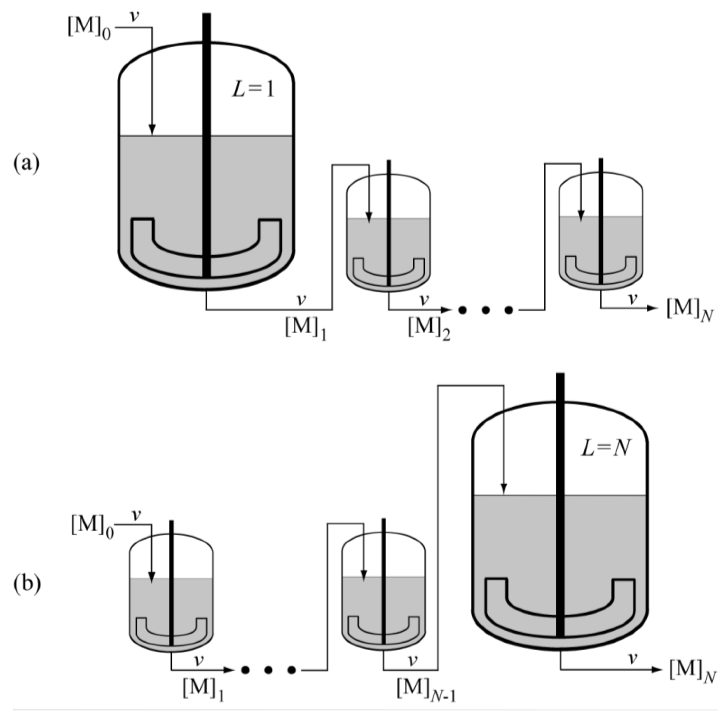
Actual MC simulation method for the tanks-in-series model is discussed in detail in references [7,18]. In this article, a series of N CSTRs, consisting of one big tank placed as the L-th tank and the same N-1 small tanks as shown in Figure 7 is considered. In the present reaction system, what is important is the magnitude of ξ, defined by the following equation, rather than the volume of reactor [7].

$${\mathsf{\xi }}_{\text{i}}=k_{\text{p},i}{[{\text{R}}^{•}]}_i{\overline{t}}_i$$

(6)

where $k_{\text{p},i}$ and ${[{\text{R}}^{•}]}_i$ are the propagation rate constant and the radical concentration both in the ith tank, and ${\overline{t}}_i$ is the mean residence time of the ith tank, i.e., ${\overline{t}}_i=V_i/v$. Here, $V_i$ is the volume of the ith tank, and v is the volumetric flow rate. By neglecting the density change, v can be considered as a constant.

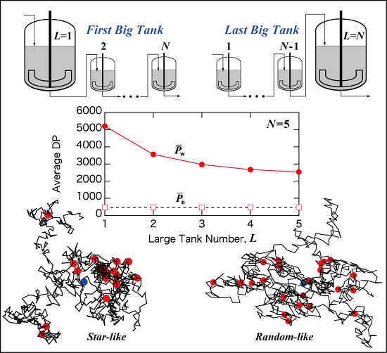
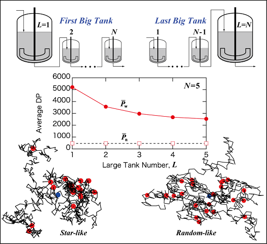
Figure 7. Illustrative representation of the N CSTRs in series, with the arrangement of (a) the first large tank L = 1; and (b) the last large tank L = N.

Figure 7. Illustrative representation of the N CSTRs in series, with the arrangement of (a) the first large tank L = 1; and (b) the last large tank L = N.

From the mathematical point of view, the cases where one large ξ-value, ξ_L with ξ_i = ξ for $i\ne L$ are discussed in this article. The value of ξ can be controlled by changing $k_{\text{p},i}$ and/or ${[{\text{R}}^{•}]}_i$, however by assuming constant values for $k_{\text{p},i}$ and ${[{\text{R}}^{•}]}_i$, the control factor is the volume of reactor V, as schematically represented by Figure 7.

Under the condition where only the L-th tank is large with the same volume for the other tanks, because every fluid element must flow through all the tanks, the residence time distribution is kept the same irrespective of the tank arrangement. In the present article, the case where the volume of one large tank is equal to the sum of other tanks, V_L = (N−1)V, is considered. 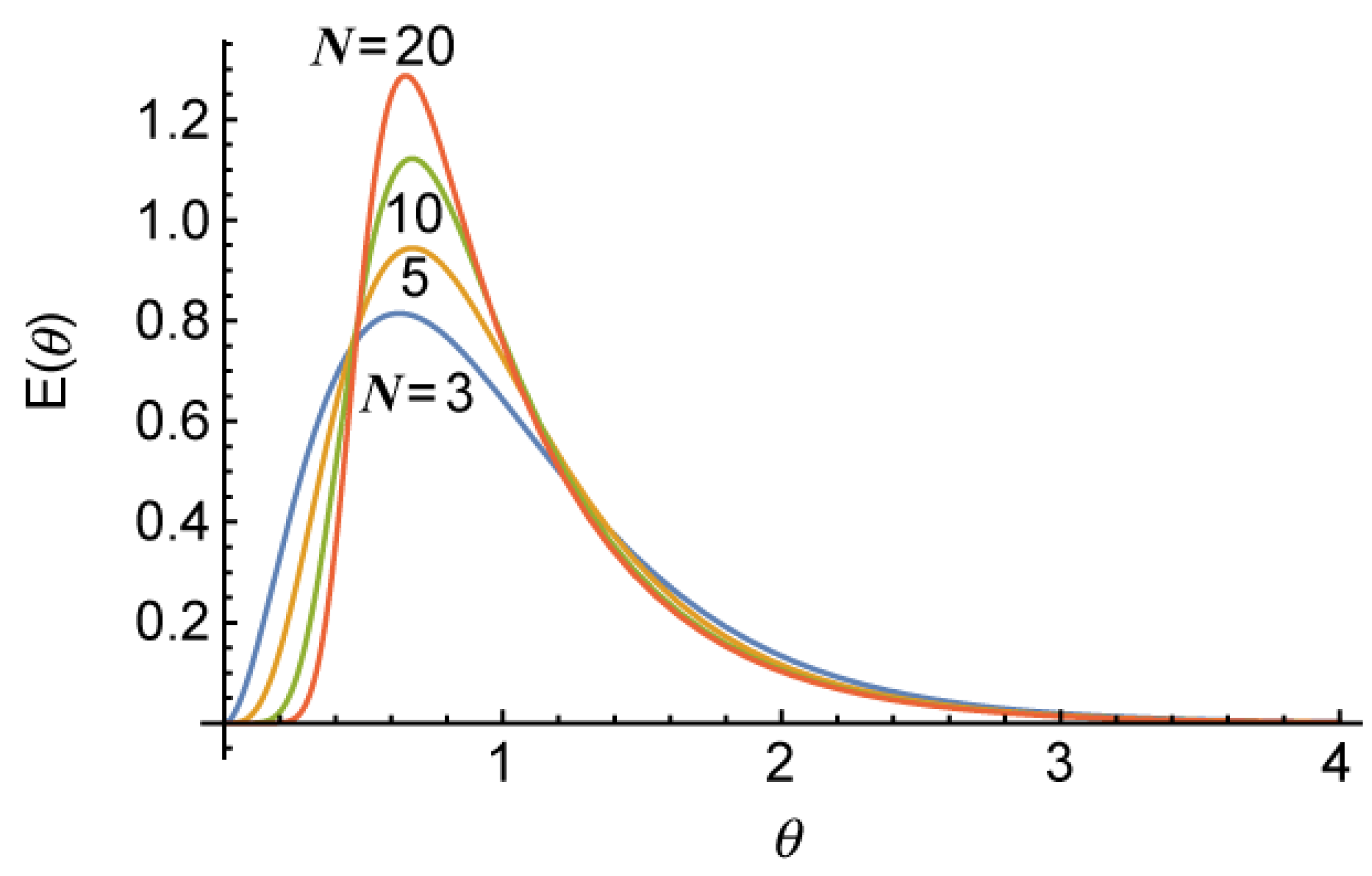In this case, the residence time distribution is shown in Figure 8 [7], where $\mathsf{\theta }=t/\overline{t}$, and $\overline{t}$ is the mean residence time of the whole reactor system. The long tail is formed due to a single large CSTR that takes up a half of total reactor volume.

Figure 8. Calculated residence time distribution for the cases with the total number of tanks, N = 3, 5, 10 and 20 [7].

Figure 8. Calculated residence time distribution for the cases with the total number of tanks, N = 3, 5, 10 and 20 [7].

In the present reactor system, the final conversion x_N, the average branching density of the product polymer ${\overline{\rho }}_N$, and the average scission density of the product polymer ${\overline{\eta }}_N$ are given, respectively, by [7]:

$$x_N=1-\frac{1}{\left(1-{\mathsf{\xi }}_L\right){\left(1-\mathsf{\xi }\right)}^{N-1}}$$

(7)

$${\overline{\rho }}_N=\frac{C_{\text{b}}}{x_N\left(1+{\mathsf{\xi }}_L\right)}\left[{\left({\mathsf{\xi }}_L\right)}^2+\mathsf{\xi }{\displaystyle \sum _{i=1}^{N-1}\left\{\left(1+{\mathsf{\xi }}_L\right)-{\left(\frac{1}{1+\mathsf{\xi }}\right)}^i\right\}}\right]$$

(8)

$${\overline{\eta }}_N=\frac{C_{\text{s}}}{x_N\left(1+{\mathsf{\xi }}_L\right)}\left[{\left({\mathsf{\xi }}_L\right)}^2+\mathsf{\xi }{\displaystyle \sum _{i=1}^{N-1}\left\{\left(1+{\mathsf{\xi }}_L\right)-{\left(\frac{1}{1+\mathsf{\xi }}\right)}^i\right\}}\right]$$

(9)

where C_b and C_s are defined respectively by C_b = k_b/k_p and C_s = k_s/k_p.

Equations (7)–(9) do not involve the large tank number L, which means that x_N, ${\overline{\rho }}_N$ and ${\overline{\eta }}_N$ do not change irrespective of the tank arrangement. The present system of CSTRs in series makes it possible to investigate the effect of tank arrangement, while keeping the following properties the same; the final conversion, the final average branching and scission densities, and the residence distribution of the whole reactor system.

3. Results and Discussion

The parameters used in the present article are shown in Table 2. The values of rate ratios, τ and β may be different depending on the tank number, however, they are assumed to be constant in the present investigation. The polymer transfer constant, C_fp = k_fp/k_p is equal to the sum of C_b and C_s, i.e., C_fp = C_b + C_s. For C3, combination termination is included. With combination termination, the crosslinks are formed, and possibility of gelation needs to be considered [24]. With C3, the value of C_s is increased to 0.005, in order to prevent gelation.

Table 2. Parameters used in the present investigation.

Parameter	C1	C3
τ = (Rtd + Rf)/Rp	0.002	0.002
β = Rtc/Rp	0	0.001
Cb = kb/kp	0.02	0.02
Cs = ks/kp	0.001	0.005

Table 2. Parameters used in the present investigation.

Parameter	C1	C3
τ = (Rtd + Rf)/Rp	0.002	0.002
β = Rtc/Rp	0	0.001
Cb = kb/kp	0.02	0.02
Cs = ks/kp	0.001	0.005

The MC simulations are conducted to generate 5 × 10⁵ polymer molecules to determine the statistical properties of the product polymers. The total number of tanks, N investigated in this study is N = 5 and 10.

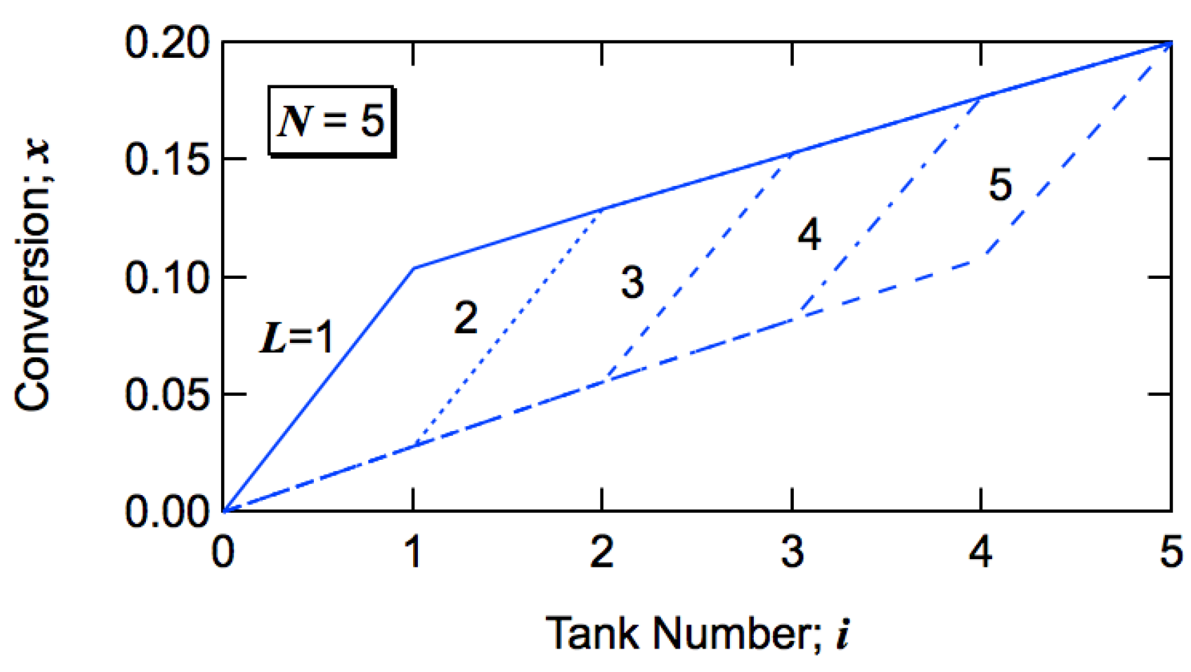
Figure 9 shows how the conversion increases with the progress of tank number for N = 5. The final conversion is set to be x_N = 0.2. For L = 1, the conversion goes up in the first tank to x₁ = 0.1035 and increases gradually to x₅ = 0.2. For L = 2, the conversion increases significantly in the second tank. Figure 10 shows the comparison with N = 10.

Figure 9. Development of monomer conversion to polymer x with the progress of tank number i for N = 5.

Figure 9. Development of monomer conversion to polymer x with the progress of tank number i for N = 5.

Figure 10. Development of monomer conversion to polymer x with the progress of tank number i for N = 5 (blue) and N = 10 (red).

Figure 10. Development of monomer conversion to polymer x with the progress of tank number i for N = 5 (blue) and N = 10 (red).

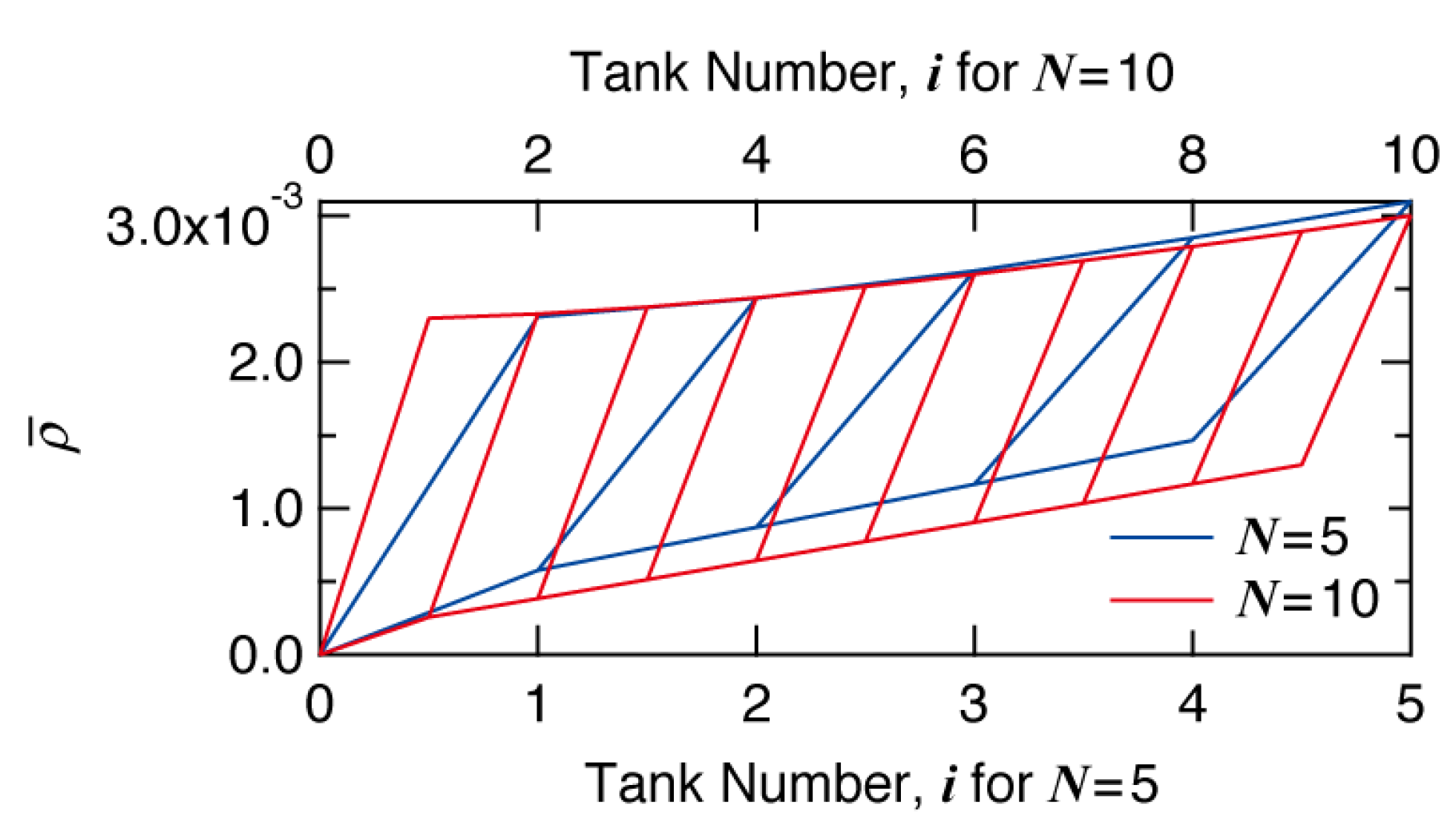
Figure 11 shows the development of average branching density $\overline{\rho }$, with the progress of tank number for N = 5 and 10. The final average branching density is slightly higher for N = 5, although the final conversion is the same. The small difference in ${\overline{\rho }}_N$ is caused by the series of small tanks part. With N = 5, there are only four small tanks, while there are nine small tanks for N = 10. Larger number of the same-sized tanks makes the behavior closer to a PFR. When the conversion level is set to be the same, a PFR leads to smaller average branching density than a series of CSTRs, as discussed in Introduction.

Figure 11. Development of average branching density $\overline{\rho }$ with the progress of tank number i for N = 5 (blue) and N = 10 (red).

Figure 11. Development of average branching density $\overline{\rho }$ with the progress of tank number i for N = 5 (blue) and N = 10 (red).

Bearing the developments of conversion and average branching density shown in Figure 10 and Figure 11 in mind, let us investigate the effect of tank arrangement on the formed branched structure.

3.1. Molecular Weight Distribution

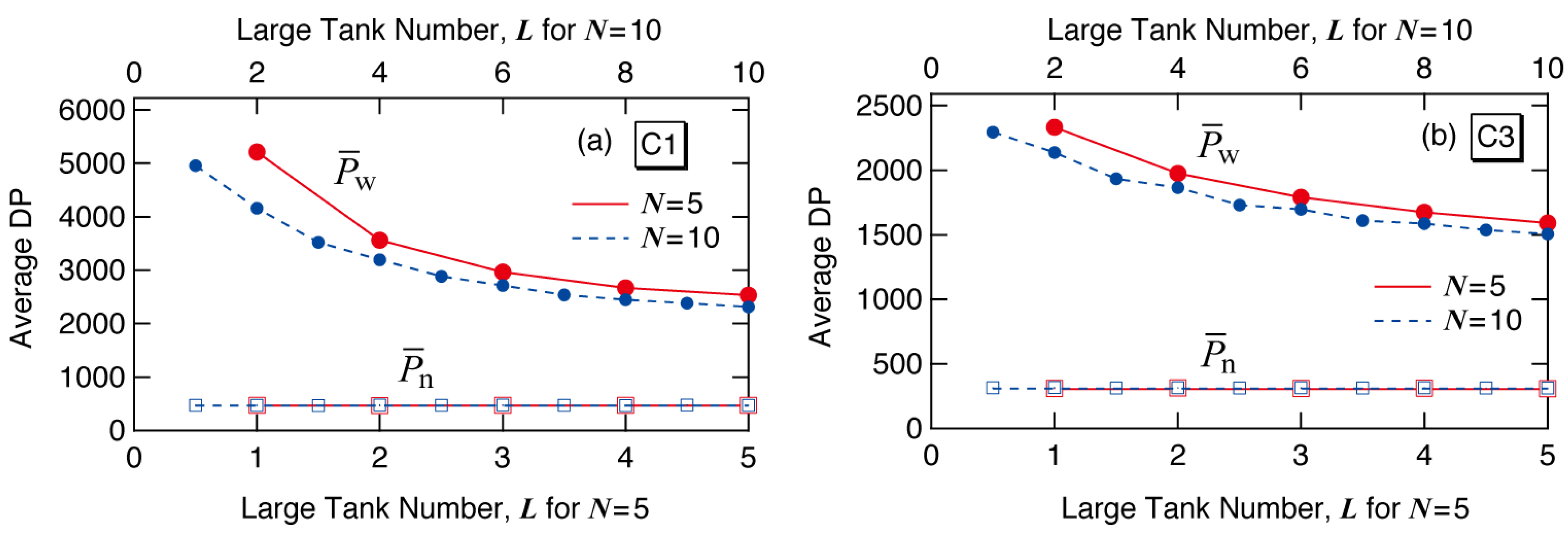
Figure 12 shows the final average degree of polymerization formed in each reactor system. The symbols are MC simulation results. The red lines and symbols are for N = 5, and the blue ones are for N = 10. The weight-average degree of polymerization, ${\overline{P}}_{\text{w}}$ is the largest for the first large tank case (L = 1), and decreases with larger L-values.

Figure 12. MC simulation results for the number (${\overline{P}}_{\text{n}}$) and weight-average (${\overline{P}}_{\text{w}}$) degree of polymerization of the polymers formed for conditions (a) C1 and (b) C3.

Figure 12. MC simulation results for the number (${\overline{P}}_{\text{n}}$) and weight-average (${\overline{P}}_{\text{w}}$) degree of polymerization of the polymers formed for conditions (a) C1 and (b) C3.

The number-average degree of polymerization, ${\overline{P}}_{\text{n}}$ is given theoretically by [18]:

$${\overline{P}}_{\text{n}}=\frac{1}{\mathsf{\tau }+\mathsf{\beta }/2+{\overline{\eta }}_N}$$

(10)

Because the final average scission density $\overline{\eta }$, as well as the values of τ and β, is the same irrespective of tank arrangement, ${\overline{P}}_{\text{n}}$ does not change with the large tank number L, as Equation (10) and the MC simulation results show.

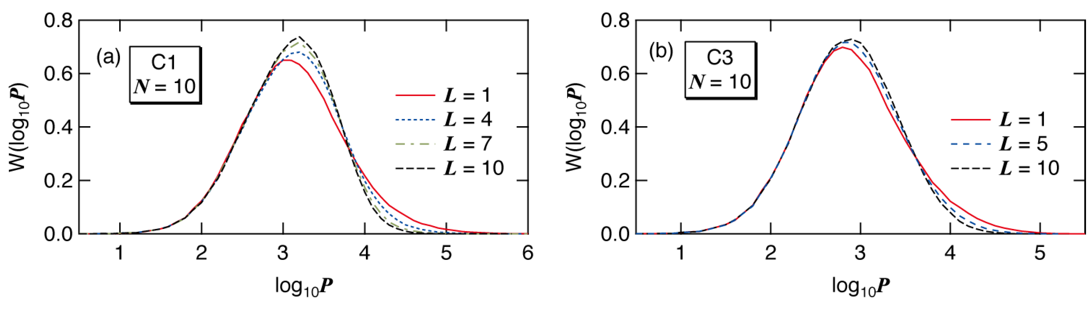
Figure 13 shows the full weight fraction distribution for N = 10. The cases with N = 5 can be found in ref. [7]. The high molecular weight tail prevails in L = 1.

Figure 13. MC simulation results for the weight fraction distribution, plotted as a function of log₁₀P, W(log₁₀P) of the polymers formed for conditions (a) C1 and (b) C3, with N = 10.

Figure 13. MC simulation results for the weight fraction distribution, plotted as a function of log₁₀P, W(log₁₀P) of the polymers formed for conditions (a) C1 and (b) C3, with N = 10.

Now, consider the qualitative explanation why the first big tank case gives the largest ${\overline{P}}_{\text{w}}$. Two important characteristics need to be reminded. The long-chain branches are formed through the polymer transfer reaction, and larger polymer molecules have a better chance of being attacked by a polymer radical. Therefore, (1) larger molecules grow faster than the smaller molecules in the present reaction system. Note that the frequency of long-chain branching is higher than that of chain scission, C_b > C_s in the present reaction system. (2) A CSTR produces broader molecular weight distribution (MWD) than that for a PFR, as shown in Figure 2. In a CSTR, the polymer molecules whose residence time is large tend to grow significantly.

Now, consider the case with L = 1. In this case, large polymer molecules are formed in the first big CSTR. After that all the polymers flow through a series of small CSTRs, which resembles a PFR. According to Item (1), larger polymer molecules grow faster in a PFR, and very large polymer molecules can be formed for the case with L = 1.

On the other hand, for the case with the last big tank, L = N, the first part is a PFR. With a PFR, the MWD surely becomes broader during polymerization, but not very much compared with a CSTR. In the final big CSTR, the MWD becomes broader, however, large polymer molecules formed before entering the last big CSTR do not necessarily stay long time in this CSTR and may not grow significantly. Therefore, the last CSTR is not very effective to make larger molecules even larger. As a result, ${\overline{P}}_{\text{w}}$ is small for the case with the last big tank, L = N.

3.2. Branching Density

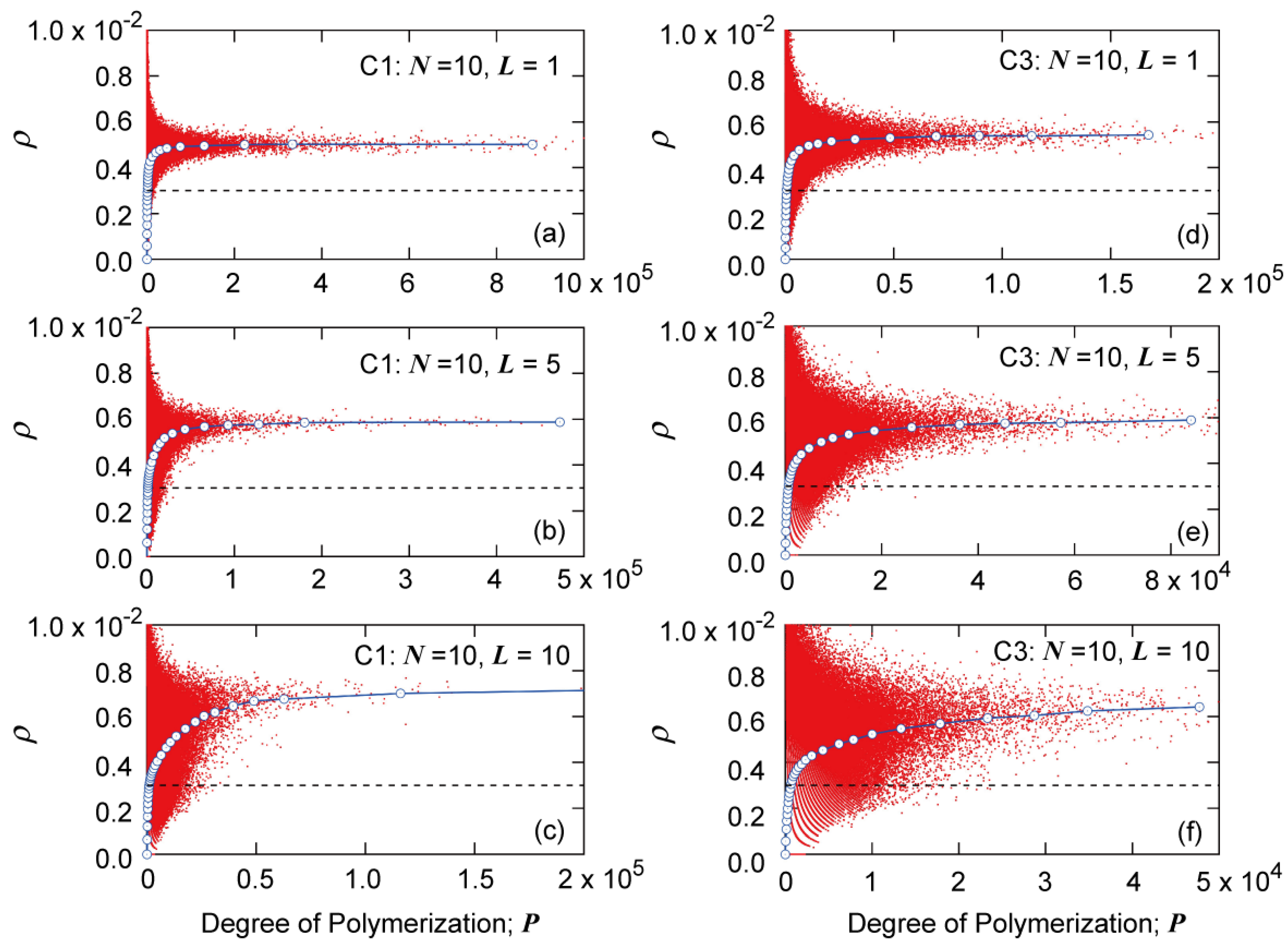
Figure 14 shows the MC simulation results for the relationship between the branching density ρ and the degree of polymerization P for N = 10. Figure 14a–c are for condition C1, and Figure 14d–f are for condition C3. The MC simulation results for N = 5 can be found in ref. [7], and the fundamental characteristics are the same as the present simulation results for N = 10. In Figure 14, each dot represents ρ and P of each polymer molecule simulated, and the solid blue curve with circular symbols shows the average branching density of polymers having degree of polymerization P, $\overline{\rho }(P)$. The dashed black line shows the average branching density of the whole system $\overline{\rho }$, which is $\overline{\rho }=0.003$ for all cases shown in Figure 14. As in the cases of other branched polymer systems, the value of $\overline{\rho }(P)$ increases with P but reaches a constant limiting value ${\rho }_{P\to \infty }$, and ${\rho }_{P\to \infty }$ is larger than the average branching density of the whole system, $\overline{\rho }$. Because the $\overline{\rho }$-value, shown by the broken line is the same, one notices that ${\rho }_{P\to \infty }$ becomes larger as the value of L increases, i.e., as the big tank moves backward.

Figure 14. Relationship between branching density ρ and degree of polymerization P, obtained from the MC simulation for N = 10: (a) C1, L = 1; (b) C1, L = 5; (c) C1, L = 10; (d) C3, L = 1; (e) C3, L = 5; and (f) C3, L = 10. The black broken line shows the average branching density of the whole reaction system, $\overline{\rho }=0.003$ for all cases.

Figure 14. Relationship between branching density ρ and degree of polymerization P, obtained from the MC simulation for N = 10: (a) C1, L = 1; (b) C1, L = 5; (c) C1, L = 10; (d) C3, L = 1; (e) C3, L = 5; and (f) C3, L = 10. The black broken line shows the average branching density of the whole reaction system, $\overline{\rho }=0.003$ for all cases.

As shown in Figure 12, the weight-average DP, ${\overline{P}}_{\text{w}}$ becomes smaller as the value of L increases. According to the present series of simulation results, ${\rho }_{P\to \infty }$ is larger for the cases that gives smaller ${\overline{P}}_{\text{w}}$. This is a completely opposite result, compared with the relationship between a PFR and a CSTR, as shown in Figure 2 and Figure 3. A CSTR gives larger ${\rho }_{P\to \infty }$ and larger ${\overline{P}}_{\text{w}}$, compared with a PFR. Now, think of the qualitative explanation for this seemingly strange conflict.

First, consider the $\overline{\rho }(P)$ curves of a CSTR and a PFR shown in Figure 3c. A larger branching density for a given degree of polymerization (P) simply means that the average chain length of the primary chains that make up a branch polymer molecule having P is smaller for a CSTR. In free-radical polymerization, each primary chain is formed within a very small time interval, and therefore, one can conveniently define the instantaneous chain length distribution [8,9]. The number-average chain length of a linear polymer radical formed through propagation starting from the time of radical generation until the dead chain formation is given by [9]:

$${\overline{P}}_{\text{n,linear}}^{•}=\frac{R_{\text{p}}}{R_{\text{td}}+R_{\text{f}}+R_{\text{tc}}+R_{\text{fp}}}=\frac{1}{\tau +\beta +R_{\text{fp}}/R_{\text{p}}}$$

(11)

In a PFR, the final term, R_fp/R_p is 0 at x = 0 because the polymer concentration is 0, and increases to the value at the final conversion, x_f. For a CSTR, R_fp/R_p is a constant, and is given by:

$$\frac{R_{\text{fp}}}{R_{\text{p}}}=C_{\text{fp}}\frac{x_{\text{f}}}{1-x_{\text{f}}}$$

(12)

where C_fp is the polymer transfer constant, and is equal to C_fp = C_b + C_s. Equation (12) represents the maximum value for a PFR reached at x_f.

The primary chain length is smaller for a CSTR. A larger number of branch points are required to form a branched polymer molecule having a given degree of polymerization, P. This is the reason for the larger $\overline{\rho }(P)$ curve of a CSTR, compared with a PFR, shown in Figure 3c.

Next, consider the CSTRs in series, with L = 1 and L = N. As shown in Figure 10, about one half of polymer by weight is formed in the large tank, and therefore, the L-th CSTR has the most important effect on the formed branched structure. The value of R_fp/R_p is C_fpx₁/(1-x₁) for L = 1, and is C_fpx_N/(1-x_N) for L = N. Because x_N > x₁, R_fp/R_p is larger for L = N, leading to give smaller primary chains for L = N. Therefore, a larger number of branch points are required to form branched polymers having a given P. The ${\rho }_{P\to \infty }$ is larger for L = N that gives smaller ${\overline{P}}_{\text{w}}$.

3.3. Radius of Gyration

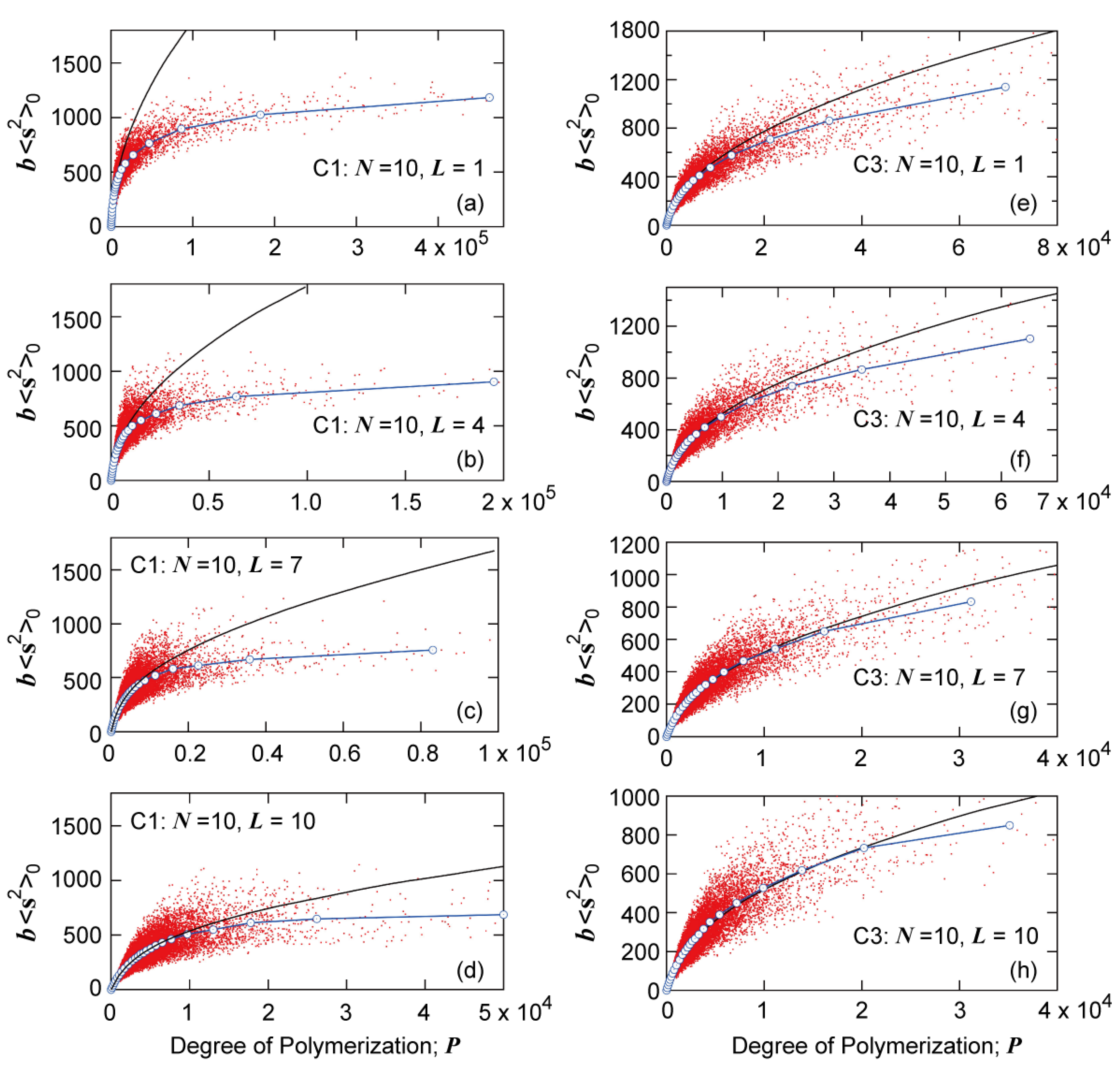
Figure 15 shows the MC simulation results for the relationship between the mean-square radius of gyration <s²>₀ and degree of polymerization P of the polymer molecules formed in various reactor placements with N = 10. Similar figures for N = 5 can be found in ref. [7]. Each dot in Figure 15 represents <s²>₀ and P-value of each polymer molecule simulated, and the blue curve with circular symbols shows the average <s²>₀ of polymers having DP, P. The black curve shows the radius of gyration of the random branched polymers given by the Zimm-Stockmayer equation [16], i.e., Equation (1). The radius of gyration is smaller than that for random branched polymers, but the degree of deviation becomes smaller as the value of L increases.

As was shown in Figure 4b, much more compact polymers are formed in a CSTR. In a CSTR, the primary polymer molecules whose residence time is large are expected to possess a larger number of branch points. These primary chains tend to form a core region of a star-like structure. This is the reason for forming compact branched polymers, especially for large polymers. On the other hand, Figure 4a shows that more randomly branched structure is tend to be formed in a PFR.

In the CSTRs in series with L = 1, compact star-like polymers are formed in the first big CSTR. After the first tank, branches are attached to the star-like polymers rather randomly, and the star-like structure is preserved, leading to form polymers with smaller <s²>₀, compared with that for random branched polymers.

Figure 15. Relationship between the mean-square radius of gyration <s²>₀ and degree of polymerization P of the polymer molecules formed in various reactor placements with N = 10: (a) C1, L = 1; (b) C1, L = 4; (c) C1, L = 7; (d) C1, L = 10; (e) C3, L = 1; (f) C3, L = 4; (g) C3, L = 7; and (h) C3, L = 10. The black curve shows the relationship for random branched polymers calculated from Equation (1).

Figure 15. Relationship between the mean-square radius of gyration <s²>₀ and degree of polymerization P of the polymer molecules formed in various reactor placements with N = 10: (a) C1, L = 1; (b) C1, L = 4; (c) C1, L = 7; (d) C1, L = 10; (e) C3, L = 1; (f) C3, L = 4; (g) C3, L = 7; and (h) C3, L = 10. The black curve shows the relationship for random branched polymers calculated from Equation (1).

Now, consider the case with the last big tank, L = N. In the first stage of N-1 small tanks, the reactor characteristics are more like a PFR, and polymers with relatively random branched structure are expected to be formed. In the final big tank, the branched polymer molecules whose residence time is large will connect many branch chains. However, looking from an entering branched polymer molecule, the branch points formed on the polymer molecule would be distributed rather randomly, and a core region will not be formed. This is the reason for obtaining polymers having relatively randomly branched polymers.

With L = 1, the branching density, ${\rho }_{P\to \infty }$ is small, as shown in Figure 14a, but much more compact polymers are formed, compared with the random branched polymers, as shown in Figure 15a. 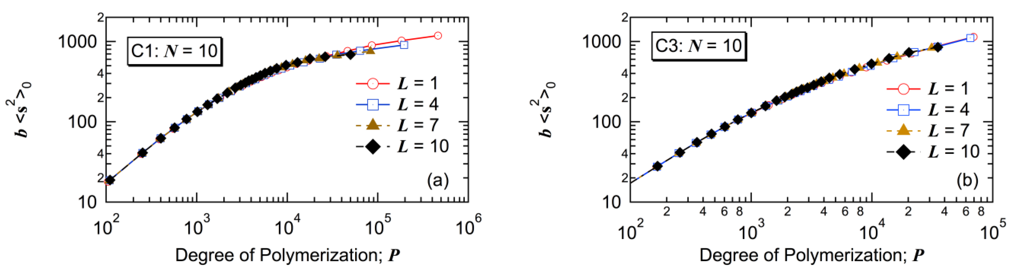On the other hand, with L = N, the branching density, ${\rho }_{P\to \infty }$ is large, as shown in Figure 14c, but the branched structure is more random and <s²>₀ is large for the given branching density level, as shown in Figure 15d. As a result, the <s²>₀-value for the given P becomes essentially the same, irrespective of the tank arrangement, as shown in Figure 16. Similarly as reported in reference [7], there seem to exist small differences for C1, but the differences are very small for C3.

Figure 16. Relationship between the mean-square radius of gyration <s²>₀ and degree of polymerization P of the polymer molecules formed with N = 10: (a) C1 and (b) C3.

Figure 16. Relationship between the mean-square radius of gyration <s²>₀ and degree of polymerization P of the polymer molecules formed with N = 10: (a) C1 and (b) C3.

4. Conclusions

In this article, a series of continuous stirred-tank reactors, consisting of one big tank and the same N-1 small tanks is investigated to design a new reactor system for free-radical polymerization with simultaneous long-chain branching and minor contribution of scission. Table 3 summarizes the results obtained in this study. When the final conversion is set to be the same, the present reactor configuration does not change the final average branching and scission densities, irrespective of the tank arrangement. The residence time distribution does not change with the tank arrangement, and therefore, the differences are not caused by the residence time distribution, but by the different history of branched polymer formation.

Table 3. N CSTRs in series with one large tank, when the final conversion, x_N, is set to be the same.

Large Tank Number, L = 1…N
Final average branching density	Unchanged
Final average scission density	Unchanged
Residence time distribution	Unchanged
Weight-average degree of polymerization, ${\overline{P}}_{\text{w}}$	>
Branching density for large polymers, ${\rho }_{P\to \infty }$	<
Branched structure	Star-like $\leftrightarrow$ Random
Relationship between <s2>0 and P	Essentially the same

Table 3. N CSTRs in series with one large tank, when the final conversion, x_N, is set to be the same.

Large Tank Number, L = 1…N
Final average branching density	Unchanged
Final average scission density	Unchanged
Residence time distribution	Unchanged
Weight-average degree of polymerization, ${\overline{P}}_{\text{w}}$	>
Branching density for large polymers, ${\rho }_{P\to \infty }$	<
Branched structure	Star-like $\leftrightarrow$ Random
Relationship between <s2>0 and P	Essentially the same

The weight-average DP, ${\overline{P}}_{\text{w}}$ is the largest for the first big tank case L = 1, and decreases as the big tank moves backward, i.e., as L increases. The branching density of large polymers, ${\rho }_{P\to \infty }$ is the smallest for L = 1, and becomes larger as L increases. With L = 1, polymers with star-like globular structure are formed. By increasing L, the polymer structure changes to a more randomly branched structure.

With L = 1, the branching density of large polymers (${\rho }_{P\to \infty }$) is small, while the structure is star-like and <s²>₀-value is small for the given branching density. On the other hand, with L = N, the branching density of large polymers (${\rho }_{P\to \infty }$) is large, while the structure is more like randomly branched and <s²>₀-value is large for the given branching density level. What is interesting is that the relationship between <s²>₀ and P is essentially unchanged by the tank arrangement.

The present investigation shows that by changing the tank arrangement, various types of branched polymers, from star-like globular structure to a more randomly branched structure, can be obtained, while keeping the followings are the same: (1) final conversion; (2) final average branching and scission densities; and (3) the relationship between <s²>₀ and P. In the case of a tower-type multi-zone reactor, the branched structure could be controlled by changing the location of division plates. On the basis of the present investigation, it is expected that the first big zone case will tend to produce polymers with star-like globular structure, while the case with the last big zone arrangement will tend to form more randomly branched polymers.

Conventionally, most mathematical models have been used to describe the behavior in the reactor that has been applied already in industry. The simulation has been used rather passively. The present type of positive use of simulation may lead to propose novel reactor systems. Table 4 highlights the characteristics of the positive model use adopted in this article.

Table 4. Positive model use proposed in this article.

Passive Model Use	Positive Model Use
Aiming at improving the process already used in industry	Aiming at creating a new process
Emphasizing the quantitative agreement with the experimental data	Emphasizing the novelty of the proposed processes
Straightforward cause-and-effect logic	Divergence through try-and-error and convergence through reasoning
Initiative by chemists	Initiative by process engineers

Table 4. Positive model use proposed in this article.

Passive Model Use	Positive Model Use
Aiming at improving the process already used in industry	Aiming at creating a new process
Emphasizing the quantitative agreement with the experimental data	Emphasizing the novelty of the proposed processes
Straightforward cause-and-effect logic	Divergence through try-and-error and convergence through reasoning
Initiative by chemists	Initiative by process engineers