Clarke-Domain Dyadic Wavelet Denoising for Three-Phase Induction Motor Current Signals

Abstract

Noise elimination in current signals of three-phase induction motors, considered as energy systems for electromechanical conversion, is a critical preprocessing step for reliable condition monitoring and fault diagnosis. However, conventional wavelet-based denoising approaches often treat noise suppression as a generic filtering task, which may distort diagnostically relevant spectral components and inter-phase relationships. To address this limitation, this paper presents a physically constrained denoising framework that integrates the Clarke transformation with dyadic wavelet analysis to enable diagnostic-safe noise attenuation. The proposed method explicitly preserves frequency bands associated with supply harmonics, mechanical phenomena, and fault-related sidebands, while enforcing inter-phase coherence and zero-sequence stability in the Clarke domain. Wavelet parameters are selected through a diagnostic-oriented multi-criteria framework that jointly balances disturbance attenuation, harmonic fidelity, coherence retention, zero-sequence stability, and time-domain waveform integrity. Experimental validation using real three-phase induction motor current measurements under steady-state conditions shows that the proposed framework achieves noise reduction ratios of approximately 8–10 dB, while preserving the amplitudes of the main harmonic components with deviations below ${10}^{-3}$ dB. These results demonstrate that the proposed method provides a robust and physically consistent preprocessing stage for current-based monitoring of three-phase AC machines.

1. Introduction

Three-phase induction motors are among the most widely used electrical machines in industrial applications due to their robustness, low cost, and high reliability [1,2]. Consequently, significant research efforts have been devoted to condition monitoring and fault diagnosis techniques [3,4,5]. Among these approaches, stator current-based methods—particularly Motor Current Signature Analysis (MCSA) have gained widespread acceptance due to their non-invasive nature, low cost, and ease of integration into existing systems [6,7,8,9,10].

Despite their widespread use, MCSA-based diagnostic methods are sensitive to measurement noise and external disturbances [11,12]. As highlighted by [13], effective fault detection depends on proper signal conditioning, since in industrial environments stator currents are often affected by high-frequency components from inverter switching, EMI, sensor limitations, grounding conditions, and acquisition systems. These disturbances reduce the detectability of fault signatures, particularly in short records or segmented signals [14]. However, signal conditioning is often treated as a secondary enhancement step rather than as a structured preprocessing framework explicitly designed for fault-oriented analysis.

Conventional noise mitigation techniques, such as fixed low-pass filtering, are often insufficient because diagnostically relevant information appears as low-amplitude sidebands and modulation components near the fundamental frequency and its harmonics [12,13]. This spectral overlap reduces the effectiveness of fixed filtering, especially under non-stationary conditions; although adaptive filtering can mitigate these limitations, it requires reference signals not always available in industrial environments [15]. Moreover, recent studies indicate that much of the undesired content in motor measurements is physically induced rather than purely stochastic, further limiting simple filtering approaches [16]. To address this, several strategies exploit the deterministic or quasi-deterministic nature of undesired components in stator currents. In particular, time-shifted and linear prediction-based approaches, including fractional-order models, have proven effective in suppressing dominant predictable components while preserving low-amplitude fault-related modulations with reduced computational complexity [17,18]. However, most reported studies treat noise attenuation as an auxiliary enhancement step rather than as a dedicated preprocessing framework with explicitly defined physical constraints. In many cases, the term “noise” is not rigorously characterized from a spectral or physical standpoint, which may lead to unintended attenuation of diagnostically relevant components [19,20,21].

In this context, multiresolution signal processing methods have gained attention for current-based diagnosis under nonstationary conditions [22,23]. The DWT enables a natural multiresolution decomposition of measured signals into approximation and detail components across dyadic scales [24,25,26], allowing selective attenuation of noise-dominated parts while preserving low-frequency content. This property has driven the adoption of wavelet-based denoising as a preprocessing stage in motor fault diagnosis [22,27,28], improving signal-to-noise ratio (SNR) and diagnostic robustness under noisy, nonstationary environments.

Noise elimination in three-phase electrical systems must attenuate high-frequency disturbances without affecting the fundamental component, low-order harmonics, or sidebands, since inadequate filtering can obscure critical diagnostic information or distort inter-phase coherence required for reliable fault detection [23]. To better meet these requirements, transforming measured currents from the phase domain into an orthogonal reference frame prior to denoising has been explored as a promising preprocessing strategy [12,29]. In particular, the Clarke Transformation (CT) maps three-phase currents into α–β–0 components [29,30,31], reducing phase redundancy, concentrating diagnostically relevant information into fewer channels, and enabling explicit handling of the zero-sequence component, often associated with common-mode disturbances and measurement artifacts. This representation has been shown to facilitate subsequent signal processing stages and improve the physical interpretability of current-based fault diagnosis [30], although its integration with systematic denoising strategies remains an open research challenge.

Although wavelet-based denoising techniques have been widely employed for noise reduction in electrical signals, most existing approaches treat denoising as a generic signal processing task, without explicitly considering the physical constraints and diagnostic relevance of three-phase electrical systems. In particular, conventional thresholding strategies may inadvertently distort harmonics, sidebands, and inter-phase relationships that are critical for condition monitoring and energy system analysis. To address this limitation, this work reformulates signal conditioning as a physically constrained preprocessing framework in the Clarke domain. By explicitly preserving frequency bands associated with electrical supply, mechanical phenomena, and fault-related components; while simultaneously enforcing inter-phase coherence and zero-sequence stability, the proposed framework ensures diagnostic-safe noise attenuation. Unlike standard denoising schemes, the method integrates physical knowledge of induction motor behavior into the wavelet-domain parameter selection, resulting in a denoising strategy that enhances signal clarity without compromising physically meaningful information.

Motivated by the need for physically consistent and diagnostically reliable preprocessing in motor current-based diagnostics, this paper proposes a noise elimination framework that integrates the Clarke transformation with band-preserving dyadic wavelet denoising to explicitly preserves diagnostically relevant spectral information prior to fault analysis.

Therefore, in this work, a diagnostic-safe, band-preserving wavelet denoising framework in the Clarke domain is introduced. In this framework, noise suppression is treated as a constrained operation that selectively attenuates high-frequency disturbances while preserving fault-related harmonics, modulation sidebands, and inter-phase consistency. Additionally, a multi-criteria wavelet parameter selection strategy is proposed. This strategy balances noise reduction with harmonic fidelity, coherence retention, zero-sequence stability, and time-domain accuracy, enabling robust preprocessing under both short-duration and long-term measurement conditions. As a result, the proposed framework provides a physically grounded and diagnostically robust preprocessing basis for subsequent fault detection and condition monitoring in three-phase induction motors and, more generally, in three-phase AC electrical machines.

The main contributions of this work are threefold: (i) the formulation of a Clarke-domain wavelet-based preprocessing framework as a physically constrained optimization problem, (ii) the explicit protection of diagnostically relevant spectral components, and (iii) the experimental validation on real three-phase induction motor current measurements. This work is organized as follows. This work is organized as follows. Section 2 presents the theoretical foundation of methodology. The Clarke-domain multiresolution wavelet denoising methodology is introduced in Section 3. In particular, the signal conditioning and Clarke-domain representation is described in Section 3.1 and the algorithms used for band-preserving wavelet denoising and for the wavelet parameter selection via multi-objective optimization are introduced in Section 3.2 and Section 3.3, respectively. The experimental setup and data acquisition are described in Section 4. Section 5 presents the results and discussion. Finally, the conclusions of this work are outlined in Section 6.

2. Theoretical Background

2.1. Clarke Transformation

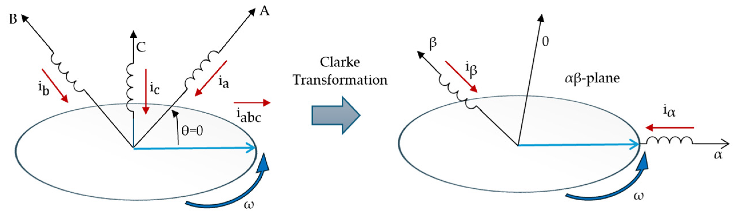
The Clarke transformation is a linear mapping that projects three-phase electrical quantities from the natural abc frame into the orthogonal stationary $\alpha \beta 0$ frame. Originally introduced by E. Clarke in the context of modified symmetrical components to simplify the analysis of unbalanced systems [32], this representation describes the spatial distribution of the three-phase system on a two-dimensional orthogonal plane through the $\alpha$ and $\beta$ components [29], while the zero-sequence component captures common-mode contributions associated with asymmetries or abnormal operating conditions. Figure 1 summarizes the coordinated transformations involved.

Figure 1. Geometric interpretation of the Clarke transformation applied to three-phase current signals.

The Clarke transformation can be derived [31] either from symmetrical component theory or from a geometric view of three-phase quantities as rotating vectors. For instantaneous phase currents ${\mathrm{i}}_{\mathrm{a}}\left(\mathrm{t}\right)$, ${\mathrm{i}}_{\mathrm{b}}\left(\mathrm{t}\right)$, and ${\mathrm{i}}_{\mathrm{c}}\left(\mathrm{t}\right)$, it is commonly expressed in matrix form as

$$\left[\begin{array}{c}{\mathrm{i}}_{\alpha }\\ {\mathrm{i}}_{\beta }\\ {\mathrm{i}}_0\end{array}\right]=\sqrt{{\displaystyle \frac{2}{3}}}\left[\begin{array}{ccc}1& -{\displaystyle \frac{1}{2}}& -{\displaystyle \frac{1}{2}}\\ 0& {\displaystyle \frac{\sqrt{3}}{2}}& -{\displaystyle \frac{\sqrt{3}}{2}}\\ {\displaystyle \frac{1}{\sqrt{2}}}& {\displaystyle \frac{1}{\sqrt{2}}}& {\displaystyle \frac{1}{\sqrt{2}}}\end{array}\right]\left[\begin{array}{c}{\mathrm{i}}_{\mathrm{a}}\\ {\mathrm{i}}_{\mathrm{b}}\\ {\mathrm{i}}_{\mathrm{c}}\end{array}\right].$$

(1)

This formulation corresponds to the power-invariant Clarke transformation [31], which preserves instantaneous power between the $\mathrm{abc}$ and $\alpha \beta 0$ frames [32]. The inverse Clarke transformation, enabling reconstruction of phase quantities from the $\alpha \beta 0$ components, is expressed as

$$\left[\begin{array}{c}{\mathrm{i}}_{\mathrm{a}}\\ {\mathrm{i}}_{\mathrm{b}}\\ {\mathrm{i}}_{\mathrm{c}}\end{array}\right]=\sqrt{{\displaystyle \frac{2}{3}}}\left[\begin{array}{ccc}1& 0& {\displaystyle \frac{1}{\sqrt{2}}}\\ -{\displaystyle \frac{1}{2}}& {\displaystyle \frac{\sqrt{3}}{2}}& {\displaystyle \frac{1}{\sqrt{2}}}\\ -{\displaystyle \frac{1}{2}}& -{\displaystyle \frac{\sqrt{3}}{2}}& {\displaystyle \frac{1}{\sqrt{2}}}\end{array}\right]\left[\begin{array}{c}{\mathrm{i}}_{\alpha }\\ {\mathrm{i}}_{\beta }\\ {\mathrm{i}}_0\end{array}\right].$$

(2)

2.2. Dyadic Wavelet Transform

The theoretical framework adopted in this work follows the wavelet frame formulation and dyadic filter bank representation previously introduced in [26]. The discrete wavelet transform (DWT) provides a multiresolution representation [24,25] of square-integrable signal $\mathrm{x}\left(\mathrm{t}\right)\in {\mathrm{L}}^2\left(\mathbb{R}\right)$ based on a wavelet family ${\left\{{\psi }_{\mathrm{j},\mathrm{k}}\left(\mathrm{t}\right)\right\}}_{\mathrm{j},\mathrm{k}\mathsf{ϵ}\mathrm{Z}},$ defined as ${\psi }_{\mathrm{j},\mathrm{k}}\left(\mathrm{t}\right)=2^{\mathrm{j}/2}\psi \left(2^{\mathrm{j}}\mathrm{t}-\mathrm{k}\right),$ where $\mathrm{j}$ and $\mathrm{k}$ denote the dyadic scale and translation parameters, respectively, and $\psi \left(\mathrm{t}\right)$ is the mother wavelet. This family forms a wavelet frame for ${\mathrm{L}}^2\left(\mathbb{R}\right)$ if there exist constants $\mathrm{A}\mathrm{and}\mathrm{B}$, known as frame bounds, such that

$$\mathrm{A}{‖\mathrm{x}‖}^2\le \sum _{\mathrm{j},\mathrm{k}}{\left|⟨\mathrm{x},{\psi }_{\mathrm{j},\mathrm{k}}⟩\right|}^2\le \mathrm{B}{‖\mathrm{x}‖}^2,0<\mathrm{A}\le \mathrm{B}<\infty$$

(3)

for all $\mathrm{x}\in {\mathrm{L}}^2\left(\mathbb{R}\right)$, where $⟨\cdot ,\cdot ⟩$ denotes the inner product in ${\mathrm{L}}^2\left(\mathbb{R}\right)$ and ${‖\mathrm{x}‖}^2$ represents the signal energy [33,34].

Multiresolution Analysis and Dyadic Decomposition

The DWT can equivalently be formulated within the multiresolution analysis (MRA) framework. In this formulation, the space ${\mathrm{L}}^2\left(\mathbb{R}\right)$ is decomposed into a nested sequence of closed subspaces ${\{\mathrm{V}}_{\mathrm{j}}{\}}_{\mathrm{j}\in \mathbb{Z}}$ satisfying [26]

$$\cdots \subset {\mathrm{V}}_{\mathrm{j}+1}\subset {\mathrm{V}}_{\mathrm{j}}\subset {\mathrm{V}}_{\mathrm{j}-1}\subset \cdots \subset {\mathrm{L}}^2(\mathbb{R}).$$

(4)

Each subspace ${\mathrm{V}}_{\mathrm{j}}$ is spanned by scaled and translated versions of a scaling function $\mathsf{\varphi }\left(\mathrm{t}\right)$. At resolution level $\mathrm{j}$, the signal $\mathrm{x}\left(\mathrm{t}\right)$ can be expressed as

$$\mathrm{x}\left(\mathrm{t}\right)=\sum _{\mathrm{k}}{\mathrm{a}}_{\mathrm{j},\mathrm{k}}{\mathsf{\varphi }}_{\mathrm{j},\mathrm{k}}\left(\mathrm{t}\right)+\sum _{\mathrm{k}}{\mathrm{d}}_{\mathrm{j},\mathrm{k}}{\psi }_{\mathrm{j},\mathrm{k}}\left(\mathrm{t}\right),$$

(5)

where ${\mathrm{a}}_{\mathrm{j},\mathrm{k}}$ and ${\mathrm{d}}_{\mathrm{j},\mathrm{k}}$ are the approximation and detail coefficients, respectively [25]. In the discrete-time domain, this dyadic decomposition admits an efficient implementation through a two-channel wavelet analysis filter bank, obtained via recursive filtering and dyadic downsampling, yielding [25,26]

$${\mathrm{a}}_{\mathrm{j}+1}\left[\mathrm{n}\right]=\sum _{\mathrm{k}}\mathrm{h}[\mathrm{k}-2\mathrm{n}]{\mathrm{a}}_{\mathrm{j}}\left[\mathrm{k}\right],{\mathrm{d}}_{\mathrm{j}+1}\left[\mathrm{n}\right]=\sum _{\mathrm{k}}\mathrm{g}[\mathrm{k}-2\mathrm{n}]{\mathrm{a}}_{\mathrm{j}}\left[\mathrm{k}\right],$$

(6)

where $\mathrm{h}[\cdot ]$ and $\mathrm{g}[\cdot ]$ are the impulse responses of the low-pass and high-pass analysis filters, respectively, and the factor of two reflects dyadic down sampling.

3. Clarke-Domain Multiresolution Wavelet Denoising Method

3.1. Signal Conditioning and Clarke-Domain Representation

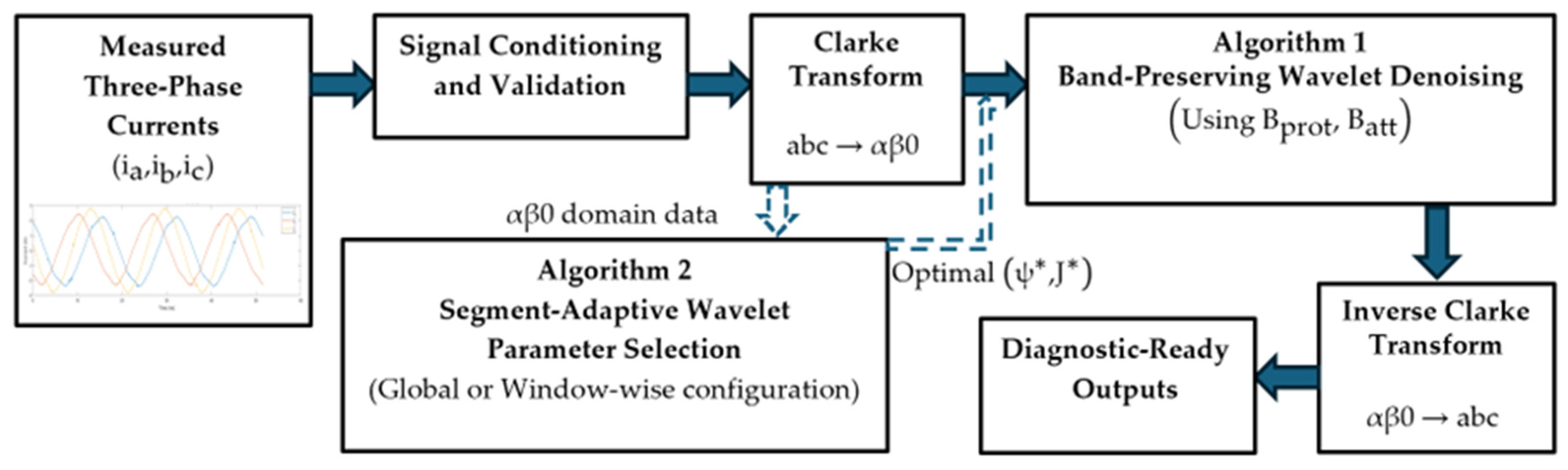
Figure 2 illustrates the block diagram of the proposed noise elimination framework. The input to the proposed framework consists of synchronously sampled three-phase stator currents ${\mathrm{i}}_{\mathrm{a}}\left(\mathrm{t}\right),{\mathrm{i}}_{\mathrm{b}}\left(\mathrm{t}\right),{\mathrm{i}}_{\mathrm{c}}\left(\mathrm{t}\right)\in {\mathrm{L}}^2(\mathbb{R})$, observed over a finite time interval $\mathrm{T}$.

Figure 2. Block diagram of the proposed Clarke-domain multiresolution wavelet denoising framework, see Algorithms 1 and 2.

Figure 2. Block diagram of the proposed Clarke-domain multiresolution wavelet denoising framework, see Algorithms 1 and 2.

Algorithm 1. Band-Preserving Wavelet Denoising

Input: Three-phase currents ${\mathrm{i}}_{\mathrm{a}},{\mathrm{i}}_{\mathrm{b}},{\mathrm{i}}_{\mathrm{c}}$; sampling frequency ${\mathrm{F}}_{\mathrm{s}}$; mother wavelet $\psi$; decomposition level J; attenuation band ${\mathrm{B}}_{\mathrm{att}}$; protected set ${\mathrm{B}}_{\mathrm{prot}}$; threshold rule (universal or SURE); shrinkage type; zero-sequence scaling ${\kappa }_0$

Output: denoised currents ${\stackrel{\mathrm{~}}{\mathrm{i}}}_{\mathrm{a}},{\stackrel{\mathrm{~}}{\mathrm{i}}}_{\mathrm{b}},{\stackrel{\mathrm{~}}{\mathrm{i}}}_{\mathrm{c}}$ and residuals ${\mathrm{r}}_{\mathrm{a}},{\mathrm{r}}_{\mathrm{b}},{\mathrm{r}}_{\mathrm{c}}$

1. Remove DC offset from ${\mathrm{i}}_{\mathrm{a}},{\mathrm{i}}_{\mathrm{b}},{\mathrm{i}}_{\mathrm{c}}$.

2. Apply Clarke transform to obtain$\left({\mathrm{i}}_{\alpha },{\mathrm{i}}_{\beta },{\mathrm{i}}_0\right)$.

3. For each component$\mathrm{x}\in \{{\mathrm{i}}_{\alpha },{\mathrm{i}}_{\beta },{\mathrm{i}}_0\}$:

1. Compute a $\mathrm{J}$-level DWT of $\mathrm{x}$.

2. Identify eligible levels${\mathrm{J}}_{\mathrm{x}}$ such that ${\mathrm{B}}_{\mathrm{j}}\subset {\mathrm{B}}_{\mathrm{att}}$ and ${\mathrm{B}}_{\mathrm{j}}\cap {\mathrm{B}}_{\mathrm{prot}}=\varnothing$.

3. For each$\mathrm{j}\in {\mathrm{J}}_{\mathrm{x}}$: estimate noise level (MAD); Compute threshold according to

selected rule; If $\mathrm{x}={\mathrm{i}}_0$, scale threshold by ${\kappa }_0$ and apply soft-thresholding.

4. Apply soft/hard shrinkage to detail coefficients at levels in${\mathrm{J}}_{\mathrm{x}}$.

5. Reconstruct$\stackrel{\mathrm{~}}{\mathrm{x}}$ via inverse DWT.

4. Apply inverse Clarke transform$\to {\stackrel{\mathrm{~}}{\mathrm{i}}}_{\mathrm{a}},{\stackrel{\mathrm{~}}{\mathrm{i}}}_{\mathrm{b}},{\stackrel{\mathrm{~}}{\mathrm{i}}}_{\mathrm{c}}$.

5. Compute residuals${\mathrm{r}}_{\mathrm{p}}={\mathrm{i}}_{\mathrm{p}}-{\stackrel{\mathrm{~}}{\mathrm{i}}}_{\mathrm{p}},\hspace{0.25em}\mathrm{p}\in \{\mathrm{a},\mathrm{b},\mathrm{c}\}$.

Algorithm 2. Segment-Adaptive Wavelet Parameter Selection

Input: ${\mathrm{i}}_{\mathrm{a}},{\mathrm{i}}_{\mathrm{b}},{\mathrm{i}}_{\mathrm{c}}$;${\mathrm{F}}_{\mathrm{s}}$; sampling frequency ${\mathrm{F}}_{\mathrm{s}}$; candidate wavelet set $\mathrm{W}$; candidate levels $\mathrm{J}$; weight vector $\mathrm{w}$; operating mode (global or window-wise).

Output: optimal parameters$\left({\psi }^{\star },{\mathrm{J}}^{\star }\right)$ (global) or $\left({\psi }_{\mathrm{s}}^{\star },{\mathrm{J}}_{\mathrm{s}}^{\star }\right)$ (window-wise)

Global mode (short record):

1. Define single segment$\mathrm{S}=1$.

2. For each$(\psi ,\mathrm{J})\in \mathrm{W}\times \mathrm{J}$:

1. Construct${\mathrm{B}}_{\mathrm{prot}}$ and ${\mathrm{B}}_{\mathrm{att}}$.

2. Apply Algorithm 1.

3. Compute metrics${\mathrm{m}}_1,\dots ,{\mathrm{m}}_5$.

4. Normalize metrics.

5. Compute score $\mathrm{S}(\psi ,\mathrm{J}).$

3. Select$\left({\psi }^{\star },{\mathrm{J}}^{\star })=\mathrm{argmax}\mathrm{S}(\psi ,\mathrm{J}\right)$.

4. Apply Algorithm 1 once using$\left({\psi }^{\star },{\mathrm{J}}^{\star }\right)$.

Window-wise mode (long record):

1. Partition signal into overlapping segments$\mathrm{s}=1,\dots ,\mathrm{S}$.

2. For each window$s$:

1. Construct${\mathrm{B}}_{\mathrm{prot}}^{\left(\mathrm{s}\right)}$$,{\mathrm{B}}_{\mathrm{att}}^{\left(\mathrm{s}\right)}$.

2. For each$(\psi ,\mathrm{J})\in {\mathrm{C}}_{\mathrm{s}}$: Apply Algorithm 1; Compute metrics${\mathrm{m}}_{\mathrm{q},\mathrm{s}}$;

Normalize metrics; Compute score${\mathrm{S}}_{\mathrm{s}}(\psi ,\mathrm{J})$.

3. Select$\left({\psi }_{\mathrm{s}}^{*},{\mathrm{J}}_{\mathrm{s}}^{*}\right)=\mathrm{argmax}{\mathrm{S}}_{\mathrm{s}}(\psi ,\mathrm{J})$.

4. Apply Algorithm 1 to segment$\mathrm{s}$.

3. Recombine denoised segments according to overlap scheme.

Prior to multiresolution processing, each phase current is conditioned by removing its DC component. In continuous time, this is defined as

$$\mathrm{a}{\stackrel{\mathrm{~}}{\mathrm{i}}}_{\mathrm{p}}\left(\mathrm{t}\right)={\mathrm{i}}_{\mathrm{p}}\left(\mathrm{t}\right)-{\displaystyle \frac{1}{\mathrm{T}}}{\int }_0^{\mathrm{T}}{\mathrm{i}}_{\mathrm{p}}\left(\tau \right)\mathrm{d}\tau ,\hspace{1em}\mathrm{p}\in \{\mathrm{a},\mathrm{b},\mathrm{c}\},$$

(7)

where $\mathrm{T}$ denotes the observation interval. For discretely sampled signals with $\mathrm{N}$ samples per phase, this operation reduces to subtracting the sample mean

$${\stackrel{\mathrm{~}}{\mathrm{i}}}_{\mathrm{p}}\left[\mathrm{n}\right]={\mathrm{i}}_{\mathrm{p}}\left[\mathrm{n}\right]-{\displaystyle \frac{1}{\mathrm{N}}}\sum _{\mathrm{m}=0}^{\mathrm{N}-1}{\mathrm{i}}_{\mathrm{p}}\left[\mathrm{m}\right],\mathrm{p}\in \{\mathrm{a},\mathrm{b},\mathrm{c}\}.$$

(8)

This conditioning avoids artificial energy concentration at very low frequencies, which is critical for spectral density estimation and wavelet analysis. The conditioned three-phase currents are then mapped to the stationary Clarke $\alpha \beta 0$ frame using the power-invariant Clarke transformation (Equation (1)), decoupling balanced components into orthogonal coordinates and enabling component-wise multiresolution processing.

3.2. Algorithm 1: Band-Preserving Wavelet Denoising

Algorithm 1 implements the physically constrained denoising stage of the proposed framework. Rather than applying wavelet thresholding indiscriminately across all resolution levels, noise suppression is formulated as a band-restricted operation in the Clarke domain. Let

$$\mathrm{x}\left(\mathrm{t}\right)\in \left\{{\mathrm{i}}_{\alpha }\left(\mathrm{t}\right),{\mathrm{i}}_{\beta }\left(\mathrm{t}\right),{\mathrm{i}}_0\left(\mathrm{t}\right)\right\}$$

(9)

denote each orthogonal Clarke-domain component obtained in Section 3.1. For a selected mother wavelet $\psi$ and decomposition level J, the discrete wavelet transform (DWT) produces approximation and detail coefficients associated with dyadic frequency bands.

Denoising is applied only to those resolution levels whose associated frequency bands do not intersect the automatically estimated set of physically meaningful spectral components. This restriction ensures that harmonic content, slip-induced sidebands, and modulation frequencies remain unaltered, while attenuation is confined to spectrally incoherent and statistically noise-dominated scales.

3.2.1. Automatic Frequency Estimation and Protected Corridor Construction

Although the proposed framework is designed for steady-state Motor Current Signature Analysis (MCSA), practical operating conditions still exhibit small deviations in the supply frequency and rotor speed due to grid fluctuations, load variations, and finite observation windows. Therefore, the methodology does not assume perfectly known harmonic, mechanical, or slip-related frequencies. Instead, these spectral landmarks are automatically estimated from the measured data within each analysis window and subsequently used to construct protected spectral corridors that enforce diagnostic-safe denoising.

Let ${\mathrm{i}}_{\mathrm{a}}\left(\mathrm{t}\right)$, ${\mathrm{i}}_{\mathrm{b}}\left(\mathrm{t}\right)$, and ${\mathrm{i}}_{\mathrm{c}}\left(\mathrm{t}\right)$ denote the measured three-phase stator currents over an analysis window. The average three-phase power spectral density (PSD) is computed using Welch’s method as [35,36]

$$\stackrel{\mathrm{-}}{\mathrm{S}}\left(\mathrm{f}\right)={\displaystyle \frac{1}{3}}\left({\mathrm{S}}_{\mathrm{a}}\left(\mathrm{f}\right)+{\mathrm{S}}_{\mathrm{b}}\left(\mathrm{f}\right)+{\mathrm{S}}_{\mathrm{c}}\left(\mathrm{f}\right)\right),$$

(10)

where ${\mathrm{S}}_{\mathrm{a}}\left(\mathrm{f}\right),{\mathrm{S}}_{\mathrm{b}}\left(\mathrm{f}\right),{\mathrm{S}}_{\mathrm{c}}\left(\mathrm{f}\right)$ are the PSDs of ${\mathrm{i}}_{\mathrm{a}}\left(\mathrm{t}\right),{\mathrm{i}}_{\mathrm{b}}\left(\mathrm{t}\right),{\mathrm{i}}_{\mathrm{c}}\left(\mathrm{t}\right)$, respectively, estimated with identical Welch parameters.

A.

Frequency-grid resolution and corridor tolerance.

Let $\Delta \mathrm{f}$denote the frequency spacing of the PSD grid, i.e.,

$$\Delta \mathrm{f}={\displaystyle \frac{{\mathrm{F}}_{\mathrm{s}}}{{\mathrm{N}}_{\mathrm{FFT}}}}\approx \mathrm{mean}(\Delta {\mathrm{f}}_{\mathrm{k}}),$$

(11)

where ${\mathrm{F}}_{\mathrm{s}}$ is the sampling frequency and ${\mathrm{N}}_{\mathrm{FFT}}$ is the FFT length used in Welch estimation. Since peak locations are subject to discretization and finite-length leakage, each protected frequency is expanded into a corridor with half-width

$$\text{∆}=2\Delta \mathrm{f}.$$

(12)

This choice ties the corridor width to the spectral resolution of the windowed PSD representation, yielding a consistent and window-adaptive tolerance without ad hoc manual tuning.

B.

Automatic estimation of ${\mathrm{f}}_{\mathrm{s}}$ and ${\mathrm{f}}_{\mathrm{r}}$ by peak tracking.

The estimated supply frequency ${\widehat{\mathrm{f}}}_{\mathrm{s}}$ is obtained by peak tracking around the nominal supply frequency ${\mathrm{f}}_{\mathrm{s},\mathrm{nom}}$ within a bounded search interval:

$${\widehat{\mathrm{f}}}_{\mathrm{s}}=\arg \underset{\mathrm{f}\in \left[{\mathrm{f}}_{\mathrm{s},\mathrm{nom}}-{\mathrm{B}}_{\mathrm{s}},{\mathrm{f}}_{\mathrm{s},\mathrm{nom}}+{\mathrm{B}}_{\mathrm{s}}\right]}{\max }\bar{\mathrm{S}}\left(\mathrm{f}\right),$$

(13)

where ${\mathrm{B}}_{\mathrm{s}}$ is a small tolerance band. Similarly, the estimated rotor mechanical frequency ${\widehat{\mathrm{f}}}_{\mathrm{r}}$ is obtained by peak tracking around the nominal mechanical frequency ${\mathrm{f}}_{\mathrm{r},\mathrm{nom}}$:

$${\widehat{\mathrm{f}}}_{\mathrm{r}}=\arg \underset{\mathrm{f}\in \left[{\mathrm{f}}_{\mathrm{r},\mathrm{nom}}-{\mathrm{B}}_{\mathrm{r}},{\mathrm{f}}_{\mathrm{r},\mathrm{nom}}+{\mathrm{B}}_{\mathrm{r}}\right]}{\max }\bar{\mathrm{S}}\left(\mathrm{f}\right),$$

(14)

with ${\mathrm{B}}_{\mathrm{r}}$ defined analogously. This window-wise estimation accommodates small speed variations while keeping the mechanical search region physically meaningful.

The search bandwidths ${\mathrm{B}}_{\mathrm{s}}$ and ${\mathrm{B}}_{\mathrm{r}}$ are chosen to exceed typical supply-frequency and speed fluctuations while remaining localized around their nominal values. In the present experiments, a tolerance of 5 Hz was adopted, which provides robust peak tracking without compromising physical interpretability.

C.

Slip estimation and protected corridor construction.

Given ${\widehat{\mathrm{f}}}_{\mathrm{s}}$, the synchronous speed is computed as

$${\widehat{\mathrm{n}}}_{\mathrm{syn}}={\displaystyle \frac{120{\widehat{\mathrm{f}}}_{\mathrm{s}}}{\mathrm{P}}},$$

(15)

where $\mathrm{P}$ denotes the number of poles. The constant 120 follows directly from the classical synchronous-speed relation of induction machines, ${\mathrm{n}}_{\mathrm{syn}}={\displaystyle \frac{120{\mathrm{f}}_{\mathrm{s}}}{\mathrm{P}}}$, expressed in revolutions per minute.

The slip estimate is then obtained from the nominal rotor speed ${\mathrm{n}}_{\mathrm{nom}}$(rpm) as

$$\widehat{\mathrm{s}}=\max \left({\displaystyle \frac{{\widehat{\mathrm{n}}}_{\mathrm{syn}}-{\mathrm{n}}_{\mathrm{nom}}}{\max \left({\widehat{\mathrm{n}}}_{\mathrm{syn}},\epsilon \right)}},0\right),$$

(16)

where $\epsilon$ prevents division by zero. The term $2\widehat{\mathrm{s}}{\widehat{\mathrm{f}}}_{\mathrm{s}}$ defines the expected slip sideband spacing around each harmonic.

Using ${\widehat{\mathrm{f}}}_{\mathrm{s}}$, ${\widehat{\mathrm{f}}}_{\mathrm{r}}$, and $\widehat{\mathrm{s}}$, the framework constructs a protected set ${\mathrm{B}}_{\mathrm{prot}}$ as a union of corridors centered at: (i) the fundamental and its harmonics, (ii) slip-related sidebands, and (iii) mechanical sidebands. For $\mathrm{k}=1,\dots ,{\mathrm{K}}_{\max }$, define the $\mathrm{k}$-th harmonic as ${\mathrm{h}}_{\mathrm{k}}=\mathrm{k}{\widehat{\mathrm{f}}}_{\mathrm{s}}$. The protected harmonic corridor is

$${\mathrm{B}}_{{\mathrm{h}}_{\mathrm{k}}}=\left[{\mathrm{h}}_{\mathrm{k}}-\text{∆},\hspace{0.25em}{\mathrm{h}}_{\mathrm{k}}+\text{∆}\right],$$

(17)

The slip-sideband corridors are

$${\mathrm{B}}_{\mathrm{sb},\mathrm{k}}=[\left({\mathrm{h}}_{\mathrm{k}}-2\widehat{\mathrm{s}}{\widehat{\mathrm{f}}}_{\mathrm{s}}\right)-\text{∆},\left({\mathrm{h}}_{\mathrm{k}}-2\widehat{\mathrm{s}}{\widehat{\mathrm{f}}}_{\mathrm{s}}\right)+\text{∆}]\cup [\left({\mathrm{h}}_{\mathrm{k}}+2\widehat{\mathrm{s}}{\widehat{\mathrm{f}}}_{\mathrm{s}}\right)-\text{∆},\left({\mathrm{h}}_{\mathrm{k}}+2\widehat{\mathrm{s}}{\widehat{\mathrm{f}}}_{\mathrm{s}}\right)+\text{∆}],$$

(18)

and the mechanical sideband corridors are

$${\mathrm{B}}_{\mathrm{mec},\mathrm{k}}=[\left({\mathrm{h}}_{\mathrm{k}}-{\widehat{\mathrm{f}}}_{\mathrm{r}}\right)-\text{∆},\left({\mathrm{h}}_{\mathrm{k}}-{\widehat{\mathrm{f}}}_{\mathrm{r}}\right)+∆]\hspace{0.25em}\cup [\left({\mathrm{h}}_{\mathrm{k}}+{\widehat{\mathrm{f}}}_{\mathrm{r}}\right)-\text{∆},\left({\mathrm{h}}_{\mathrm{k}}+{\widehat{\mathrm{f}}}_{\mathrm{r}}\right)+\text{∆}].$$

(19)

Finally, the overall protected set is defined as

$${\mathrm{B}}_{\mathrm{prot}}={\bigcup }_{\mathrm{k}=1}^{{\mathrm{k}}_{\max }}\left({\mathrm{B}}_{{\mathrm{h}}_{\mathrm{k}}}\cup {\mathrm{B}}_{\mathrm{sb},\mathrm{k}}\cup {\mathrm{B}}_{\mathrm{mec},\mathrm{k}}\right).$$

(20)

The set B defines a physics-driven spectral protection mask that preserves harmonics, slip-related sidebands, and mechanically induced modulation components. It does not assume where noise is located; rather, it constrains subsequent denoising operations to avoid distortion of diagnostically interpretable spectral structures. In this study, harmonics up to ${\mathrm{K}}_{\max }=13$ are considered, although the framework admits arbitrary ${\mathrm{K}}_{\max }$ depending on the spectral richness and diagnostic requirements of the target system.

3.2.2. Dyadic Frequency Localization and Data-Driven Attenuation Band

For a sampling frequency ${\mathrm{F}}_{\mathrm{s}}$, the discrete wavelet transform decomposes each Clarke-domain component into approximation and detail coefficients associated with dyadic frequency intervals. Under standard multiresolution analysis assumptions, the detail coefficients at level $\mathrm{j}$ are approximately associated with the frequency band [25,33].

$${\mathrm{B}}_{\mathrm{j}}\approx \left[{\displaystyle \frac{{\mathrm{F}}_{\mathrm{s}}}{2^{\mathrm{j}+1}}},{\displaystyle \frac{{\mathrm{F}}_{\mathrm{s}}}{2^{\mathrm{j}}}}\right],$$

(21)

which provides an approximate mapping between wavelet scales and spectral regions. Unlike conventional approaches that assume noise to be confined to a predetermined high-frequency range, the proposed framework identifies attenuation-eligible spectral regions in a data-driven manner.

Let $\bar{\mathrm{S}}\left(\mathrm{f}\right)$ denote the segment-wise average three-phase PSD defined in (10) and let $\mathrm{C}\left(\mathrm{f}\right)$ denote the average inter-phase magnitude-squared coherence. The attenuation candidate band ${\mathrm{B}}_{\mathrm{att}}\subset [0,{\mathrm{F}}_{\mathrm{s}}/2]$ is defined as a contiguous spectral interval satisfying:

$${\mathrm{B}}_{\mathrm{att}}=\left[{\mathrm{f}}_{\mathrm{att},1},{\mathrm{f}}_{\mathrm{att},2}\right],$$

(22)

subject to the following constraints:

• Non-intersection with the protected set:

$${\mathrm{B}}_{\mathrm{att}}\cap {\mathrm{B}}_{\mathrm{prot}}=\varnothing ,$$

2.

Reduced three-phase coherence:

$$\mathrm{C}\left(\mathrm{f}\right)<{\tau }_{\mathrm{c}},\text{∀}\mathrm{f}\in {\mathrm{B}}_{\mathrm{att}},$$

3.

Absence of dominant structured peaks in $\bar{\mathrm{S}}\left(\mathrm{f}\right)$.

The coherence threshold ${\tau }_{\mathrm{c}}$ and peak-dispersion criteria are selected to isolate broadband, weakly structured spectral content while excluding harmonically organized components.

This formulation ensures that attenuation is not imposed on a fixed frequency range, but rather on spectral regions that are (i) physically unprotected and (ii) spectrally incoherent.

Once ${\mathrm{B}}_{\mathrm{att}}$ is determined, the dyadic bands ${\mathrm{B}}_{\mathrm{j}}$ are evaluated against both ${\mathrm{B}}_{\mathrm{prot}}$ and ${\mathrm{B}}_{\mathrm{att}}$. The statistical validation of noise-dominated behavior for these candidate scales is introduced in the following subsection.

3.2.3. Statistical Noise Characterization in the Wavelet Domain

After identifying the attenuation-eligible spectral region ${\mathrm{B}}_{\mathrm{att}}$ and mapping dyadic bands ${\mathrm{B}}_{\mathrm{j}}$, noise-dominated behavior is defined operationally through statistical properties of the wavelet detail coefficients.

Let

$${\mathrm{D}}_{\mathrm{j}}=\{{\mathrm{d}}_{\mathrm{j},\mathrm{n}}{\}}_{\mathrm{n}=1}^{{\mathrm{N}}_{\mathrm{j}}}$$

denote the set of detail coefficients at level $\mathrm{j}$, where ${\mathrm{N}}_{\mathrm{j}}$ is the number of coefficients at that resolution.

A level $\mathrm{j}$ is considered statistically analyzable if

$${\mathrm{B}}_{\mathrm{j}}\cap {\mathrm{B}}_{\mathrm{att}}\ne \varnothing \wedge {\mathrm{B}}_{\mathrm{j}}\cap {\mathrm{B}}_{\mathrm{prot}}=\varnothing .$$

(23)

For such levels, a robust dispersion estimate is computed using the median absolute deviation (MAD):

$$\widehat{{\sigma }_{\mathrm{j}}}={\displaystyle \frac{\mathrm{median}\left(\left|{\mathrm{D}}_{\mathrm{j}}-\mathrm{median}\left({\mathrm{D}}_{\mathrm{j}}\right)\right|\right)}{0.6745}}.$$

(24)

The scaling factor 0.6745 corresponds to the inverse of the 75th percentile of the standard normal distribution and provides a robust scale estimate comparable to the standard deviation. Owing to its resistance to outliers and structured components, the estimator remains reliable under non-Gaussian conditions.

To assess distributional symmetry and tail behavior, higher-order statistics are computed:

$${\gamma }_{\mathrm{j}}=\mathrm{skew}\left({\mathrm{D}}_{\mathrm{j}}\right),{\kappa }_{\mathrm{j}}=\mathrm{kurt}\left({\mathrm{D}}_{\mathrm{j}}\right).$$

(25)

Under noise-dominated behavior, coefficients are expected to exhibit near symmetry and absence of structured heavy tails:

$$\left|{\gamma }_{\mathrm{j}}\right|\approx 0,{\kappa }_{\mathrm{j}}\approx 3.$$

(26)

Normality consistency is further assessed using the Jarque–Bera statistic:

$$\mathrm{J}{\mathrm{B}}_{\mathrm{j}}={\displaystyle \frac{{\mathrm{N}}_{\mathrm{j}}}{6}}\left({\gamma }_{\mathrm{j}}^2+{\displaystyle \frac{{\left({\kappa }_{\mathrm{j}}-3\right)}^2}{4}}\right),$$

(27)

which asymptotically follows a ${\chi }_2^2$ distribution under the null hypothesis of normality. A wavelet level is considered statistically consistent with noise-dominated behavior if

$$\mathrm{J}{\mathrm{B}}_{\mathrm{j}}\le {\chi }_{2,\alpha }^2.$$

(28)

Importantly, Gaussianity is not imposed as a strict requirement for attenuation. Instead, the statistical descriptors serve to verify the absence of structured deterministic signatures typically associated with harmonics, modulation components, or fault-induced spectral lines.

3.2.4. Constrained Thresholding Strategy

Once a resolution level $\mathrm{j}$ satisfies both the spectral admissibility condition (Section 3.2.2) and the statistical noise-consistency criteria (Section 3.2.3), attenuation is applied to the corresponding wavelet detail coefficients.

Let ${\mathrm{d}}_{\mathrm{j}}\left[\mathrm{n}\right]$, $\mathrm{n}=1,\dots ,{\mathrm{N}}_{\mathrm{j}}$, denote the detail coefficients at level $\mathrm{j}$, and let ${\widehat{\sigma }}_{\mathrm{j}}$ be the robust scale estimate defined in (24). Thresholding is restricted to resolution levels belonging to the set

$${\mathrm{J}}_{\mathrm{den}}=\{\mathrm{j}\in \{1,\dots ,\mathrm{J}\left\}:\left({\mathrm{B}}_{\mathrm{j}}\cap {\mathrm{B}}_{\mathrm{att}}\ne \varnothing \right)\wedge \left({\mathrm{B}}_{\mathrm{j}}\cap {\mathrm{B}}_{\mathrm{prot}}=\varnothing \right)\right\},$$

(29)

which coincides with the statistically validated admissible levels introduced in (23).

This formulation guarantees that attenuation is applied to dyadic levels whose bands intersect the data-driven attenuation region ${\mathrm{B}}_{\mathrm{att}}$ while remaining strictly outside the protected corridors ${\mathrm{B}}_{\mathrm{prot}}$.

A.

Threshold Selection Criteria.

Two complementary threshold selection strategies are considered to assess the stability of the proposed framework under conservative and data-adaptive shrinkage regimes.

(1) Universal (Donoho-Type) Threshold [37,38].

The universal threshold is defined as

$${\lambda }_{\mathrm{j}}^{\left(\mathrm{univ}\right)}={\widehat{\sigma }}_{\mathrm{j}}\sqrt{2\ln ({\mathrm{N}}_{\mathrm{j}})},$$

(30)

where ${\mathrm{N}}_{\mathrm{j}}$ is the number of coefficients at level $\mathrm{j}$.

The universal rule is asymptotically minimax optimal under independent noise assumptions and provides strong suppression of stochastic disturbances. However, it is known to be conservative and may induce over-smoothing when the signal-to-noise ratio is moderate.

(2) SURE-Based Threshold [37].

To mitigate the conservativeness of the universal rule, a Stein’s Unbiased Risk Estimator (SURE)-based threshold is also evaluated:

$${\lambda }_{\mathrm{j}}^{\left(\mathrm{SURE}\right)}=\arg \underset{\lambda \text{≥}0}{\min }{\mathrm{SURE}}_{\mathrm{j}}\left(\lambda \right),$$

(31)

where ${\mathrm{SURE}}_{\mathrm{j}}(\lambda )$ provides an unbiased estimate of the mean squared reconstruction error associated with soft-thresholding.

Unlike the universal threshold, the SURE rule adapts to the empirical distribution of the coefficients and may produce milder attenuation in the presence of low-energy structured content.

Although classical thresholding rules are derived under Gaussian assumptions, their application here is strictly confined to statistically validated noise-dominated levels.

• B. Component-Dependent Scaling.

To account for the distinct physical interpretation of Clarke-domain components, a component-dependent scaling factor ${\kappa }_{\mathrm{x}}$, with $\mathrm{x}\in \{\alpha ,\beta ,0\}$, is introduced:

$${\lambda }_{\mathrm{j},\mathrm{x}}={\kappa }_{\mathrm{x}}{\lambda }_{\mathrm{j}}.$$

(32)

For the orthogonal components,

$${\kappa }_{\alpha }={\kappa }_{\beta }=1,$$

(33)

while for the zero-sequence component,

$${\kappa }_0=1+{\alpha }_{\kappa }{\displaystyle \frac{\mathrm{RMS}\left({\mathrm{i}}_0\right)}{\max \left(\mathrm{RMS}\left({\mathrm{i}}_{\alpha },{\mathrm{i}}_{\beta }\right),\epsilon \right)}}.$$

(34)

This proportional scaling reflects the relative contribution of zero-sequence energy to segment-level asymmetry. Consequently, additional attenuation is applied only when the zero-sequence component exhibits significant energy outside the protected spectral corridors, reinforcing suppression of asymmetry-sensitive content without altering physically meaningful components.

• C. Soft-Threshold Operator.

For $\mathrm{j}\in {\mathrm{J}}_{\mathrm{den}}$, soft-thresholding is applied as

$${\stackrel{\mathrm{~}}{\mathrm{d}}}_{\mathrm{j}}\left[\mathrm{n}\right]=\mathrm{sign}\left(\mathrm{dj}\left[\mathrm{n}\right]\right)\max \left(\left|{\mathrm{d}}_{\mathrm{j}}\left[\mathrm{n}\right]\right|-{\lambda }_{\mathrm{j},\mathrm{x}},0\right),$$

(35)

which preserves continuity of the shrinkage function and reduces reconstruction artifacts compared to hard thresholding.

For $\mathrm{j}\notin {\mathrm{J}}_{\mathrm{den}}$,

$${\stackrel{\mathrm{~}}{\mathrm{d}}}_{\mathrm{j}}\left[\mathrm{n}\right]=\mathrm{dj}\left[\mathrm{n}\right].$$

(36)

• D. Inverse Reconstruction

The denoised Clarke-domain component is reconstructed via the inverse discrete wavelet transform:

$$\stackrel{\mathrm{~}}{\mathrm{x}}\left(\mathrm{t}\right)=\mathrm{iDWT}\left({\mathrm{x}}_{\mathrm{A}}^{\left(\mathrm{J}\right)}\left(\mathrm{t}\right),\{{\tilde{\mathrm{x}}}_{\mathrm{D}}^{\left(\mathrm{j}\right)}\left(\mathrm{t}\right){\}}_{\mathrm{j}=1}^{\mathrm{J}}\right).$$

(37)

Finally, the denoised three-phase currents are obtained through the inverse Clarke transformation.

3.3. Algorithm 2: Segment-Adaptive Wavelet Parameter Selection via Normalized Multi-Metric Optimization

The physically constrained denoising stage (Algorithm 1) requires two structural parameters: the mother wavelet $\psi$ and the decomposition level $\mathrm{J}$. While Algorithm 1 enforces diagnostic-safe thresholding by restricting attenuation to eligible dyadic bands, the resulting performance still depends on the chosen $\left(\psi ,\mathrm{J}\right)$, since the time–frequency localization, regularity, and phase response of the wavelet family directly affect the distribution of wavelet coefficients and the reconstruction behavior.

Operating modes. Algorithm 2 supports two operational configurations. For short-duration or quasi-stationary signals, the entire record constitutes a single segment ($\mathrm{S}=1$), and a global optimal pair $\left({\psi }^{*},{\mathrm{J}}^{*}\right)$ is selected and applied over the full observation interval. For long-duration or nonstationary signals, the measured current record is partitioned into overlapping analysis windows (segments) indexed by $\mathrm{s}\in \{1,\dots ,\mathrm{S}\}$. In this adaptive configuration, the optimal pair $\left({\psi }_{\mathrm{s}}^{*},{\mathrm{J}}_{\mathrm{s}}^{*}\right)$ is determined independently for each segment.

All spectral quantities, protected corridors, attenuation bands, and evaluation metrics are computed consistently within each segment. This segment dependency is explicitly denoted using the superscript $\left(\mathrm{s}\right)$, which is omitted when $\mathrm{S}=1$ without loss of generality.

3.3.1. Candidate Set Definition and Structural Feasibility

Let $\mathrm{W}$ denote the finite set of candidate mother wavelets (spanning different families and regularities) and let $\mathrm{J}$ denote the set of admissible decomposition levels. For a segment $s$ containing ${\mathrm{N}}_{\mathrm{s}}$ samples, the feasible candidate set is defined as

$${\mathrm{C}}_{\mathrm{s}}=\left\{\left(\psi ,\mathrm{J}\right):\psi \in \mathrm{W},\mathrm{J}\in \mathrm{J},2^{\mathrm{J}}\le {\displaystyle \frac{{\mathrm{N}}_{\mathrm{s}}}{8}}\right\}.$$

(38)

The feasibility constraint $2^{\mathrm{J}}\le {\mathrm{N}}_{\mathrm{s}}/8$ prevents unstable decompositions in which the coarsest scale would be supported by an insufficient number of samples. In practice, this avoids degenerate cases where the approximation coefficients at level $\mathrm{J}$ become too few to support reliable reconstruction and to preserve inter-phase structural information.

3.3.2. Segment-Wise Denoising and Performance Metrics

For each candidate pair $(\psi ,\mathrm{J})\in {\mathrm{C}}_{\mathrm{s}}$, Algorithm 1 is applied using the segment-specific protected corridors and attenuation band, i.e., ${\mathrm{B}}_{\mathrm{prot}}^{\left(\mathrm{s}\right)}$ (constructed in Section 3.2.1) and ${\mathrm{B}}_{\mathrm{att}}^{\left(\mathrm{s}\right)}$ (identified in Section 3.2.2):

$${\stackrel{\mathrm{~}}{\mathrm{i}}}_{\mathrm{abc}}^{\left(\mathrm{s}\right)}\left(\mathrm{t};\psi ,\mathrm{J}\right)=\mathrm{Alg}1\left({\mathrm{i}}_{\mathrm{abc}}^{\left(\mathrm{s}\right)}\left(\mathrm{t}\right);\psi ,\mathrm{J},{\mathrm{B}}_{\mathrm{att}}^{\left(\mathrm{s}\right)},{\mathrm{B}}_{\mathrm{prot}}^{\left(\mathrm{s}\right)}\right).$$

(39)

The denoised output is then evaluated using complementary metrics designed to quantify three competing objectives: (i) attenuation of disturbance-dominated content, (ii) preservation of protected spectral structures, and (iii) integrity of three-phase structure and waveform shape. All metrics below are computed within the same segment $\mathrm{s}$.

A.

Attenuation performance (broadband suppression).

Let ${\bar{\mathrm{S}}}_{\mathrm{raw}}^{\left(\mathrm{s}\right)}\left(\mathrm{f}\right)$ and ${\bar{\mathrm{S}}}_{\mathrm{den}}^{\left(\mathrm{s}\right)}\left(\mathrm{f}\right)$ denote the segment-wise average three-phase PSDs (computed as in (10) before and after denoising). The attenuation-band power is defined as

$${\mathrm{P}}_{\mathrm{att},*}^{\left(\mathrm{s}\right)}={\int }_{{\mathrm{B}}_{\mathrm{att}}^{\left(\mathrm{s}\right)}}{\bar{\mathrm{s}}}_{*}^{\left(\mathrm{s}\right)}\left(\mathrm{f}\right)\mathrm{df},*\in \{\mathrm{raw},\mathrm{den}\}.$$

(40)

The attenuation benefit metric (noise-reduction ratio in the attenuation band) is

$${\mathrm{m}}_{1,\mathrm{s}}\left(\psi ,\mathrm{J}\right)={\mathrm{NRR}}_{\mathrm{att}}^{\left(\mathrm{s}\right)}=10{\log }_{10}\left({\displaystyle \frac{{\mathrm{P}}_{\mathrm{att},\mathrm{raw}}^{\left(\mathrm{s}\right)}}{\max \left({\mathrm{P}}_{\mathrm{att},\mathrm{den}}^{\left(\mathrm{s}\right)},\epsilon \right)}}\right).$$

(41)

This metric quantifies broadband suppression inside ${\mathrm{B}}_{\mathrm{att}}^{\left(\mathrm{s}\right)}$ without assuming that “noise lives at high frequency”; instead, it measures how effectively the method reduces power in the data-driven attenuation region defined by coherence and peak-dispersion criteria (Section 3.2.2).

B.

Protected spectral fidelity (local distortion control).

Let the protected set be expressed as a union of corridors:

$${\mathrm{B}}_{\mathrm{prot}}^{\left(\mathrm{s}\right)}={\bigcup }_{\mathrm{k}=1}^{\mathrm{K}}{\mathrm{B}}_{\mathrm{k}}^{\left(\mathrm{s}\right)}.$$

For each corridor ${\mathrm{B}}_{\mathrm{k}}^{\left(\mathrm{s}\right)}$, the protected power before and after denoising is

$${\mathrm{P}}_{\mathrm{k},*}^{\left(\mathrm{s}\right)}={\int }_{{\mathrm{B}}_{\mathrm{k}}^{\left(\mathrm{s}\right)}}{\bar{\mathrm{s}}}_{*}^{\left(\mathrm{s}\right)}\left(\mathrm{f}\right)\mathrm{df},*\in \{\mathrm{raw},\mathrm{den}\}.$$

(42)

The relative corridor distortion is defined as

$${\epsilon }_{\mathrm{k}}^{\left(\mathrm{s}\right)}={\displaystyle \frac{\left|{\mathrm{P}}_{\mathrm{k},\mathrm{den}}^{\left(\mathrm{s}\right)}-{\mathrm{P}}_{\mathrm{k},\mathrm{raw}}^{\left(\mathrm{s}\right)}\right|}{\max \left({\mathrm{P}}_{\mathrm{k},\mathrm{raw}}^{\left(\mathrm{s}\right)},\epsilon \right)}}.$$

(43)

Two aggregated fidelity metrics are then used:

$${\mathrm{m}}_{2,\mathrm{s}}\left(\psi ,\mathrm{J}\right)={\displaystyle \frac{1}{\mathrm{K}}}\sum _{\mathrm{k}=1}^{\mathrm{K}}{\epsilon }_{\mathrm{k}}^{\left(\mathrm{s}\right)},{\mathrm{m}}_{3,\mathrm{s}}\left(\psi ,\mathrm{J}\right)=\underset{\mathrm{k}}{\max }{\epsilon }_{\mathrm{k}}^{\left(\mathrm{s}\right)}.$$

(44)

Here, ${\mathrm{m}}_{2,\mathrm{s}}$ captures average preservation across all protected corridors, while $m_{3,s}$ enforces a conservative bound that penalizes any local over-smoothing that may destroy a specific diagnostic feature (e.g., a weak sideband corridor).

C.

Inter-phase coherence consistency (structural coupling).

Let ${\gamma }_{\mathrm{raw}}^{2,\left(\mathrm{s}\right)}\left(\mathrm{f}\right)$ and ${\gamma }_{\mathrm{den}}^{2,\left(\mathrm{s}\right)}\left(\mathrm{f}\right)$ denote the segment-wise average magnitude-squared coherence (computed over phase pairs and averaged, as in the implementation). The coherence over the protected set is

$${\mathsf{\Gamma }}_{\mathrm{prot},*}^{\left(\mathrm{s}\right)}={\displaystyle \frac{1}{\left|{\mathrm{B}}_{\mathrm{prot}}^{\left(\mathrm{s}\right)}\right|}}{\int }_{{\mathrm{B}}_{\mathrm{prot}}^{\left(\mathrm{s}\right)}}{\gamma }_{*}^{2,\left(\mathrm{s}\right)}\left(\mathrm{f}\right)\mathrm{df},\mathrm{*}\in \{\mathrm{raw},\mathrm{den}\}.$$

(45)

The coherence deviation metric is

$${\mathrm{m}}_{4,\mathrm{s}}\left(\psi ,\mathrm{J}\right)=\left|{\mathsf{\Gamma }}_{\mathrm{prot},\mathrm{den}}^{\left(\mathrm{s}\right)}-{\mathsf{\Gamma }}_{\mathrm{prot},\mathrm{raw}}^{\left(\mathrm{s}\right)}\right|$$

(46)

This term prevents candidate solutions that reduce disturbances at the cost of breaking the intrinsic three-phase coupling and phase-to-phase consistency.

D.

Time-domain waveform integrity (distortion control).

For each phase $\mathrm{p}\in \{\mathrm{a},\mathrm{b},\mathrm{c}\}$, the segment-wise RMSE is

$${\mathrm{RMSE}}_{\mathrm{p}}^{\left(\mathrm{s}\right)}=\sqrt{{\displaystyle \frac{1}{{\mathrm{N}}_{\mathrm{s}}}}\sum _{\mathrm{n}=1}^{{\mathrm{N}}_{\mathrm{s}}}{\left({\stackrel{\mathrm{~}}{\mathrm{i}}}_{\mathrm{p}}^{\left(\mathrm{s}\right)}\left[\mathrm{n}\right]-{\mathrm{i}}_{\mathrm{p}}^{\left(\mathrm{s}\right)}\left[\mathrm{n}\right]\right)}^2}.$$

(47)

The average waveform distortion metric is

$${\mathrm{m}}_{5,\mathrm{s}}\left(\psi ,\mathrm{J}\right)={\displaystyle \frac{1}{3}}\sum _{\mathrm{p}\in \left\{\mathrm{a},\mathrm{b},\mathrm{c}\right\}}{\mathrm{RMSE}}_{\mathrm{p}}^{\left(\mathrm{s}\right)}.$$

(48)

This term penalizes excessive time-domain smoothing and protects the overall current waveform shape, complementing the purely spectral criteria.

3.3.3. Segment-Wise Min–Max Normalization (Scale-Free Ranking)

Because ${\{\mathrm{m}}_{\mathrm{q},\mathrm{s}}{\}}_{\mathrm{q}=1}^5$ have heterogeneous units and ranges, direct scalarization would be dominated by the metric with the largest numerical spread. Therefore, each metric is normalized within each segment $s$ over the candidate set ${\mathrm{C}}_{\mathrm{s}}$ using min–max normalization:

$${\overline{\mathrm{m}}}_{\mathrm{q},\mathrm{s}}\left(\psi ,\mathrm{J}\right)={\displaystyle \frac{{\mathrm{m}}_{\mathrm{q},\mathrm{s}}\left(\psi ,\mathrm{J}\right)-{\mathrm{m}}_{\mathrm{q},\mathrm{s}}^{\min }}{{\mathrm{m}}_{\mathrm{q},\mathrm{s}}^{\max }-{\mathrm{m}}_{\mathrm{q},\mathrm{s}}^{\min }+\epsilon }},\mathrm{q}=1,\dots ,5,$$

(49)

where

$${\mathrm{m}}_{\mathrm{q},\mathrm{s}}^{\min }=\underset{\left(\psi ,\mathrm{J}\right)\in {\mathrm{C}}_{\mathrm{s}}}{\min }{\mathrm{m}}_{\mathrm{q},\mathrm{s}}\left(\psi ,\mathrm{J}\right),{\mathrm{m}}_{\mathrm{q},\mathrm{s}}^{\max }=\underset{\left(\psi ,\mathrm{J}\right)\in {\mathrm{C}}_{\mathrm{s}}}{\max }{\mathrm{m}}_{\mathrm{q},\mathrm{s}}\left(\psi ,\mathrm{J}\right).$$

The small constant $\epsilon >0$ prevents division by zero when ${\mathrm{m}}_{\mathrm{q},\mathrm{s}}^{\max }={\mathrm{m}}_{\mathrm{q},\mathrm{s}}^{\min }$ (e.g., when a metric is constant across candidates in a specific segment). This segment-wise normalization yields a relative ranking that is comparable across metrics within the same segment and prevents scale dominance, while preserving the local decision structure of each window.

3.3.4. Scalarization and Optimal Selection Rule

The selection of $\left(\psi ,\mathrm{J}\right)$ is formulated as a scalarized multi-objective optimization. Since ${\mathrm{m}}_{1,\mathrm{s}}$ is beneficial (higher is better) while ${\mathrm{m}}_{2,\mathrm{s}}$–${\mathrm{m}}_{5,\mathrm{s}}$ are penalty-like (lower is better), the segment-wise score function is defined as

$${\mathrm{S}}_{\mathrm{s}}\left(\psi ,\mathrm{J}\right)={\mathrm{w}}_1{\overline{\mathrm{m}}}_{1,\mathrm{s}}\left(\psi ,\mathrm{J}\right)-\sum _{\mathrm{q}=2}^5{\mathrm{w}}_{\mathrm{q}}{\overline{\mathrm{m}}}_{\mathrm{q},\mathrm{s}}\left(\psi ,\mathrm{J}\right),$$

(50)

with nonnegative weights satisfying

$${\mathrm{w}}_{\mathrm{q}}\ge 0,\sum _{\mathrm{q}=1}^5{\mathrm{w}}_{\mathrm{q}}=1.$$

(51)

The optimal pair is selected as

$$\left({\psi }^{\star },{\mathrm{J}}^{\star }\right)=\arg \underset{(\psi ,\mathrm{J}),\in {\mathrm{C}}_{\mathrm{s}}}{\max }{\mathrm{S}}_{\mathrm{s}}\left(\psi ,\mathrm{J}\right).$$

(52)

Because all terms are normalized within $\left[0,1\right]$ (up to $\epsilon$), the score in (50) implements a balanced trade-off between attenuation strength and preservation constraints. Moreover, given a fixed candidate set ${\mathrm{C}}_{\mathrm{s}}$, fixed normalization rule (49), and fixed weights ${\mathrm{w}}_{\mathrm{q}}$, the selection (52) is fully deterministic and reproducible.

3.3.5. Weight Selection, Interpretability, and Robustness

The weights ${\mathrm{w}}_1,\dots ,{\mathrm{w}}_5$ in (50) encode the relative preference between suppression and preservation objectives. They do not modify the denoising operator in Algorithm 1; they only affect how candidate pairs $\left(\psi ,\mathrm{J}\right)$ are ranked.

A.

Origin and rationale of weights.

In this work, the weights are chosen to reflect the methodological goal of “diagnostic-safe preprocessing”: attenuation is desirable, but only insofar as protected spectral structures, three-phase coupling, and waveform integrity remain stable. This is implemented by assigning the largest weight to attenuation (${\mathrm{w}}_1$) while distributing the remaining weight among preservation penalties (${\mathrm{w}}_2$–${\mathrm{w}}_5$). The base configuration is

$${\mathrm{w}}^{\left(0\right)}=\left[{\mathrm{w}}_1,{\mathrm{w}}_2,{\mathrm{w}}_3,{\mathrm{w}}_4,{\mathrm{w}}_5\right]={\displaystyle \frac{\left[1.0,1.0,0.5,0.5,0.5\right]}{{\sum }_{\mathrm{q}=1}^5{\mathrm{w}}_{\mathrm{q}}}},$$

(53)

i.e., normalized to satisfy (51). This choice is consistent with a conservative diagnostic objective: ${\mathrm{m}}_{2,\mathrm{s}}$ and ${\mathrm{m}}_{3,\mathrm{s}}$ jointly protect spectral corridors, while ${\mathrm{m}}_{4,\mathrm{s}}$ and ${\mathrm{m}}_{5,\mathrm{s}}$ enforce structural and waveform constraints.

B.

Non-subjectivity via sensitivity analysis.

To address potential subjectivity in $\left({\psi }_{\mathrm{s}}^{*},{\mathrm{J}}_{\mathrm{s}}^{*}\right)$, the framework evaluates multiple weight configurations $\left\{{\mathrm{w}}^{\left(\mathrm{l}\right)}\right\}$ and quantifies the stability of the selected solution under preference perturbations. Specifically, the implementation tests four weight sets: (i) a base configuration, (ii) stronger attenuation emphasis, (iii) stronger preservation emphasis, and (iv) stronger time-domain integrity emphasis. Consistent selection across these sets indicates that $\left({\psi }_{\mathrm{s}}^{\star },{\mathrm{J}}_{\mathrm{s}}^{\star }\right)$ is not an artifact of a single subjective weight choice but a robust outcome driven by the candidate landscape and the normalized multi-metric structure.

C.

Practical interpretation.

The optimization in (52) should be interpreted as selecting the wavelet configuration that yields the best compromise between removing incoherent disturbance-dominated energy (as defined by ${\mathrm{B}}_{\mathrm{att}}^{\left(\mathrm{s}\right)}$) and preserving diagnostically interpretable spectral and structural features (as enforced by ${\mathrm{B}}_{\mathrm{prot}}^{\left(\mathrm{s}\right)}$, coherence stability, and RMSE).

For clarity and reproducibility, the procedures of Algorithms 1 and 2 are summarized below in pseudocode form.

3.4. Baseline Methods and Benchmark Protocol

To objectively assess the effectiveness of the proposed band-preserving wavelet framework, several baseline denoising strategies were implemented under controlled and comparable conditions. All baselines were executed on the same analysis segments and using the same automatically estimated supply frequency, rotor frequency, slip, protected corridors ${\mathrm{B}}_{\mathrm{prot}}^{\left(\mathrm{s}\right)}$, and attenuation band ${\mathrm{B}}_{\mathrm{att}}^{\left(\mathrm{s}\right)}$, whenever applicable, to ensure a fair comparison.

3.4.1. Butterworth Bandstop Filtering

A classical digital Butterworth band-stop filter was implemented as a linear filtering baseline. The stopband limits were defined using the automatically identified attenuation band ${\mathrm{B}}_{\mathrm{att}}^{\left(\mathrm{s}\right)}$ (see Equation (22)).

The normalized digital cutoff frequencies were computed as

$${\omega }_{1,2}^{\left(\mathrm{s}\right)}={\displaystyle \frac{2{\mathrm{f}}_{\mathrm{att},1,2}^{\left(\mathrm{s}\right)}}{{\mathrm{F}}_{\mathrm{s}}}}.$$

(54)

A fourth-order IIR Butterworth filter was designed using bilinear transformation, ensuring monotonic passband and stopband behavior without ripple [39,40]. Unlike the proposed framework, no explicit protected spectral corridors were enforced beyond the inherent frequency response of the filter.

Structural Limitation. Although Butterworth filtering constitutes a stable and widely validated linear framework, it inherently depends on the explicit specification of stop-band limits. In practical applications, the choice of cutoff frequencies often requires heuristic decisions or preliminary spectral inspection to identify disturbance-dominated regions [41]. Under nonstationary operating conditions, these fixed limits may cease to be optimal over time, leading to either insufficient attenuation or distortion of diagnostically relevant spectral components [41,42]. This dependence on predefined parameters represents a fundamental limitation of classical fixed-parameter filtering approaches.

3.4.2. Wavelet Shrinkage—Optimized (WS-Optimized)

A wavelet shrinkage method was implemented using the optimal parameter pair $\left({\psi }^{*},{\mathrm{J}}^{*}\right)$ obtained from Algorithm 2. However, unlike the proposed band-preserving framework, thresholding was applied uniformly across all dyadic levels [38] without enforcing the protected-set constraint ${\mathrm{B}}_{\mathrm{prot}}^{\left(\mathrm{s}\right)}$.

Noise level estimation was performed using the median absolute deviation (MAD) estimator, and thresholding was applied using the same shrinkage rule adopted in the proposed method.

This baseline isolates the benefit of the multi-metric parameter selection while removing the physics-driven band restriction.

3.4.3. Wavelet Shrinkage—Fixed (WS-Fixed)

A conventional wavelet denoising configuration was implemented using a fixed mother wavelet and decomposition level [25]:

$$\psi =\mathrm{db}8,\mathrm{J}=5.$$

Thresholding was applied to all detail levels using soft-thresholding with MAD-based noise estimation. No adaptive parameter selection or spectral band restriction was applied. This baseline represents a commonly adopted fixed-configuration wavelet denoising strategy.

3.4.4. Empirical Mode Decomposition (EMD)

An empirical mode decomposition (EMD) denoising strategy was implemented by reconstructing the signal after discarding the first $\tau =3$ intrinsic mode functions (IMFs), assumed to capture disturbance-dominated components [43,44].

No explicit spectral protection mechanism was enforced. The method operates purely in the time domain based on adaptive mode decomposition.

3.4.5. Benchmark Protocol

All methods were evaluated using the same performance metrics defined in Section 3.3:

• ${\mathrm{m}}_{1,\mathrm{s}}$: attenuation performance within ${\mathrm{B}}_{\mathrm{att}}^{\left(\mathrm{s}\right)}$;

• ${\mathrm{m}}_{2,\mathrm{s}}$, ${\mathrm{m}}_{3,\mathrm{s}}$: protected spectral fidelity;

• ${\mathrm{m}}_{4,\mathrm{s}}$: inter-phase coherence consistency;

• ${\mathrm{m}}_{5,\mathrm{s}}$: time-domain waveform integrity.

This unified evaluation protocol ensures that performance differences are attributed to methodological distinctions rather than discrepancies in parameter estimation, segmentation, or evaluation criteria.

4. Experimental Setup and Data Acquisition

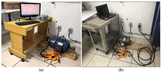
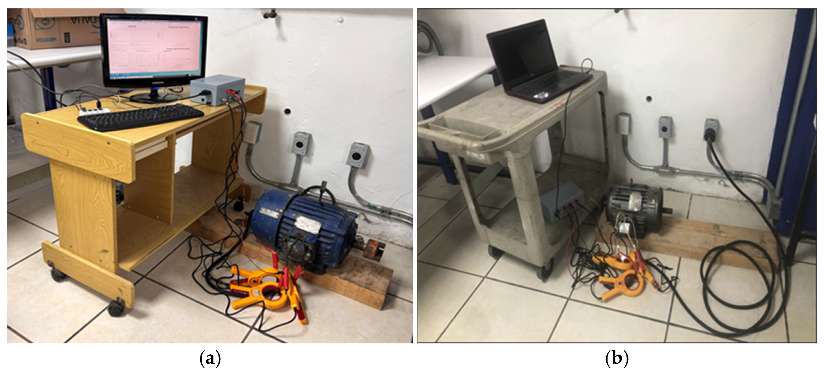
The experimental validation was conducted under controlled steady-state operating conditions using two independent three-phase squirrel-cage induction motors. The objective of the experimental design was to evaluate the proposed preprocessing framework under quasi-stationary current regimes typically encountered in industrial monitoring applications. Transient startup conditions and load oscillations were intentionally excluded, since the proposed methodology is specifically designed for steady-state Motor Current Signature Analysis (MCSA), where spectral fault-related components are spectrally stable and physically interpretable. Figure 3 illustrates the complete experimental arrangement used in this study, including the induction motors under test, non-intrusive current sensing devices, and the FPGA-based data acquisition platform.

Figure 3. Experimental setups for stator current acquisition under steady-state operation: (a) U.S. Electrical Motors 215T (3 HP, 1740 rpm) used for the long-duration dataset; (b) Baldor M3661T (3 HP, 1750 rpm) used for the short-duration dataset.

4.1. Induction Motors Under Test

Two induction motors were employed in the experimental validation, corresponding to the long-duration and short-duration acquisition scenarios.

The first motor, used for the long-duration dataset, is a three-phase squirrel-cage induction motor (U.S. Electrical Motors, Waukesha, WI, USA), frame 215T, rated at 3 HP, 60 Hz, and 1740 rpm under nominal load. The machine operates at a synchronous speed of 1800 rpm and exhibits typical industrial slip characteristics. It is designed for 230/460 V operation and insulation Class F.The second motor, used for the short-duration dataset, is a three-phase induction motor (Baldor Electric Company, Fort Smith, AR, USA), model M3661T, rated at 3 HP, 60 Hz, and 1750 rpm, with a NEMA 182TC frame. The nominal mechanical rotational frequency is approximately 29.17 Hz. In both cases, the motors were supplied directly from the electrical grid without inverter-based control or external drive electronics. This configuration ensures that the measured stator currents contain supply-related and electromechanical spectral components representative of industrial steady-state operation.

4.2. Data Acquisition Hardware and Signal Conditioning

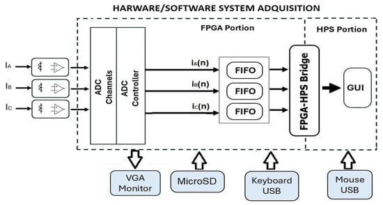
Figure 4 presents a simplified block diagram of the developed hardware–software acquisition platform.

Figure 4. Simplified block diagram of the developed hardware–software data acquisition system.

Three-phase stator currents ia(t), ib(t), and ic(t) were measured using split-core clamp-type current sensors (ETCR070A, ETCR, Guangzhou, China), providing galvanic isolation and enabling non-intrusive acquisition without interrupting the power circuit. The sensors deliver secondary outputs proportional to the primary current, with standardized 1 A or 5 A outputs over a nominal measurement range of 0–1000 A (AC). The operating frequency range spans from 40 Hz to 1 kHz. The motors were directly connected to the electrical grid and operated under steady-state conditions without inverter-based drives or external control electronics. Consequently, the measured currents represent grid-supplied industrial operation. The secondary current signals were conditioned using an INA114 instrumentation amplifier (Texas Instruments, Dallas, TX, USA) to match the input range of the acquisition system [45]. Signals were digitized by a multi-channel ADC and buffered in FIFO memories.

Data handling was implemented on a Terasic DE10-Nano platform (Terasic Technologies, Hsinchu, Taiwan) incorporating a Cyclone V SoC-FPGA (Intel Corporation, Santa Clara, CA, USA). The FPGA side performs synchronized sampling and buffering, while the Hard Processor System (HPS) manages data transfer and real-time visualization through a LabVIEW-based graphical interface (National Instruments, Austin, TX, USA). The FPGA clock was set to 50 MHz, ensuring stable and synchronized multi-channel acquisition.

The FPGA platform was exclusively used for synchronized multi-channel current acquisition and real-time visualization. It does not perform motor control functions.

4.3. Acquired Signals and Measurement Scenarios

Two stator current datasets were acquired for each motor to evaluate the proposed methodology under different signal-duration and sampling conditions. Experiments were performed independently on both induction machines under controlled steady-state operation.

For the short-duration scenario, 768 samples per phase were acquired at a sampling frequency of 14,880 Hz. This configuration captures approximately three electrical cycles and represents short observation windows typically encountered in embedded monitoring systems and early-stage diagnostic applications.

For the long-duration scenario, approximately 31,000 samples per phase were acquired at a sampling frequency of 3000 Hz. This dataset reflects quasi-stationary operating conditions and is used to assess the robustness and consistency of the proposed framework over extended observation intervals through window-based analysis.

In all cases, three-phase stator currents were synchronously acquired and processed using the proposed preprocessing framework.

5. Results and Discussion

5.1. Short-Signal Analysis

The first scenario used a short-duration current signal acquired from the Baldor induction motor under steady-state operating conditions. In healthy operation, the stator current spectrum is dominated by the supply fundamental, its harmonics, and modulation sidebands associated with rotor slip and mechanical interactions. These components constitute the diagnostic basis for fault detection; therefore, the preprocessing stage must attenuate broadband disturbances without compromising their spectral integrity. The performance of the proposed approach was compared with the reference techniques described in the previous sections.

5.1.1. Short-Signal Denoising Performance

Table 1 and Table 2 summarize the denoising performance obtained using the Universal and SURE threshold rules, respectively. Under the Universal configuration (Table 1), the method achieves an attenuation level of ${\mathrm{NRR}}_{\mathrm{att}}=8.948\pm 0.757\mathrm{d}$B, whereas the SURE configuration (Table 2) yields ${\mathrm{NRR}}_{\mathrm{att}}=4.570\pm 0.247\mathrm{d}$B. Although these values are lower than those obtained with the Butterworth band-stop filter ($17.713\pm 5.358$ dB), the difference reflects their distinct design philosophies. Butterworth maximizes attenuation by aggressively rejecting energy within a predefined stopband, whereas the proposed framework intentionally limits attenuation to avoid distortion of diagnostically relevant spectral components.

Table 1. Denoising performance using the Universal threshold rule.

Method	NRR_att (dB)	$\rho$_prot	errProt_max	ΔCoh_prot	RMSE_avg
Proposed	8.948 ± 0.757	1 ± 8.5866 × 10−7	2.8004 × 10−6 ± 8.5866 × 10−7	−0.003496 ± 0.0027039	0.12888 ± 0.15456
Butterworth-BS	17.713 ± 5.358	1 ± 1.7337 × 10−7	3.9739 × 10−6 ± 1.7337 × 10−7	0.00040821 ± 0.00032969	0.12017 ± 0.143
WS-Optimized	6.912 ± 1.476	0.99987 ± 2.8273 × 10−5	0.00013224 ± 2.8273 × 10−5	0.037418 ± 0.055438	0.31883 ± 0.41608
WS-Fixed	7.095 ± 1.499	0.999 ± 0.0002274	0.00099656 ± 0.0002274	−0.12556 ± 0.027276	0.79071 ± 1.0325
EMD	1.396 ± 1.220	1.0001 ± 0.00042887	0.00014717 ± 0.00014717	−0.030775 ± 0.027103	0.043733 ± 0.037122

Table 2. Denoising performance using the SURE threshold rule.

Method	NRR_att (dB)	$\rho$_prot	errProt_max	ΔCoh_prot	RMSE_avg
Proposed	4.570 ± 0.247	1 ± 1.1708 × 10−6	2.398 e−06 ± 1.1708 × 10−6	−0.0026072 ± 0.0045049	0.094845 ± 0.11437
Butterworth-BS	17.713 ± 5.358	1 ± 1.7337 × 10−7	3.9739 × 10−6± 1.7337 × 10−7	0.00040821 ± 0.00032969	0.12017 ± 0.143
WS-Optimized	6.912 ± 1.476	0.99987 ± 2.8273 × 10−5	0.00013224 ± 2.8273 × 10−5	0.037418 ± 0.055438	1.4332 ± 1.9911
WS-Fixed	7.095 ± 1.499	0.999 ± 0.0002274	0.00099656 ± 0.0002274	−0.12556 ± 0.027276	0.79071 ± 1.0325
EMD	1.396 ± 1.220	1.0001 ± 0.00042887	0.00030325 ± 0.00014717	−0.037577 ± 0.027103	0.047531 ± 0.031751

This behavior is reflected in preservation metrics. The protected energy ratio ${\rho }_{\mathrm{prot}}$ remains equal to unity for both configurations ($1\pm 8.6\times {10}^{-7}$ for Universal and $1\pm 1.17\times {10}^{-6}$ for SURE), indicating nearly perfect conservation of spectral energy within the protected corridors. Similarly, the maximum distortion in the protected region remains extremely small, with ${\mathrm{errProt}}_{\max }$ values of approximately $2.8\times {10}^{-6}$ and $2.39\times {10}^{-6}$ for the Universal and SURE rules, respectively. In contrast, the wavelet shrinkage baselines introduce distortions two to three orders of magnitude larger, reaching $1.3\times {10}^{-4}$ for WS-Optimized and nearly ${10}^{-3}$ for WS-Fixed.

The coherence preservation metric $\Delta {\mathrm{Coh}}_{\mathrm{prot}}$ further supports this behavior. The proposed method maintains coherence variations close to zero ($-0.0035$ and $-0.0026$ for Universal and SURE), indicating that the phase relationships between stator currents remain essentially unchanged after denoising. By contrast, WS-Fixed produces a much larger deviation (−$0.12556$), revealing significant perturbation of spectral coupling between phases.

A similar trend is observed in the waveform distortion metric ${\mathrm{RMSE}}_{\mathrm{avg}}$. The SURE configuration yields the lowest distortion among the wavelet-based approaches (0.094845), compared with 0.12888 for the Universal rule and substantially larger values for WS-Optimized (1.4332) and WS-Fixed (0.79071). These results indicate that the proposed method removes disturbance-dominated components while preserving the global waveform characteristics of the signal.

5.1.2. Optimal Parameter Configuration

The optimal parameter configurations selected by the proposed framework are summarized in Table 3. In the first run, both threshold rules converged to the same configuration, selecting the Symlet wavelet $\mathrm{sym}9$ with decomposition level $\mathrm{J}=4$. In the second run, the framework selected the Coiflet wavelet $\mathrm{coif}5$, while maintaining the same decomposition level.

Table 3. Parameter configuration of the proposed method for the analyzed runs.

Run	Threshold	$\mathrm{Wavelet}(\psi$)	Level (J)	${\mathbf{f}}_{\mathbf{s}}\left(\mathbf{Hz}\right)$	${\mathbf{f}}_{\mathbf{r}}\left(\mathbf{Hz}\right)$	Slip	${\mathbf{B}}_{\mathbf{att}}$(Hz)	${\mathbf{k}}_0$
1	UNIVERSAL	Sym9	4	60	29.33	0.0222	[1000, 7000]	3.078
1	SURE	Sym9	4	60	29.33	0.0222	[1000, 7000]	3.078
2	UNIVERSAL	coif5	4	60	29.33	0.0222	[1000, 7000]	1.787
2	SURE	coif5	4	60	29.33	0.0222	[1000, 7000]	1.787

Two key characteristics of the optimization strategy emerge. First, strong intra-run consistency is observed: within each run, the optimal wavelet and decomposition level remain identical for both threshold rules, indicating that the multiresolution structure is primarily determined by the spectral characteristics of the signal rather than by the thresholding rule. Second, inter-run adaptability appears, as the optimal wavelet changes from Symlet to Coiflet while the decomposition level remains fixed, confirming that the framework does not assume a single wavelet basis to be universally optimal.

The physical parameters estimated by the framework remain stable across runs. The supply frequency is consistently identified as ${\mathrm{f}}_{\mathrm{s}}=60$ Hz, the rotor mechanical frequency as ${\mathrm{f}}_{\mathrm{r}}=29.33\mathrm{Hz}$, and the slip as $\mathrm{s}=0.0222$, values consistent with the operating conditions of the Baldor motor. The automatically detected attenuation band ${\mathrm{B}}_{\mathrm{a}\mathrm{t}\mathrm{t}}=\left[\mathrm{1000,\; 7000}\right]\mathrm{H}\mathrm{z}$ lies well above the fundamental harmonic region.

5.1.3. Harmonic and Sideband Preservation

The preservation of harmonic and sideband components is analyzed in Table 4, which reports the spectral deviations after denoising for the main diagnostic frequencies. For the fundamental component ${\mathrm{H}}_1$ and its associated sidebands ${\mathrm{H}}_1\pm {\mathrm{f}}_{\mathrm{r}}$ and ${\mathrm{H}}_1\pm 2\mathrm{s}{\mathrm{f}}_{\mathrm{s}}$, the proposed framework produces essentially zero spectral deviation for both threshold rules, with variations remaining within numerical precision (≈0 dB). This confirms that the fundamental harmonic structure of the stator current is almost perfectly preserved after denoising, validating the effectiveness of the protected spectral corridors defined by the framework.

Table 4. Spectral deviation (Δ dB) of harmonic and sideband components after denoising relative to the original signal.

Spectral Component	${\mathbf{f}}_0\left(\mathbf{Hz}\right)$	$\mathbf{Raw}\text{\_}\mathbf{dB}$	$\Delta \mathbf{Proposed}$ $\mathbf{UNIVERSAL}$ (dB)	Δ Proposed SURE (dB)	Δ Butter (dB)	Δ WS-Opt (dB)	Δ WS-Fix (dB)	Δ EMD (dB)
${\mathrm{H}}_1$	60	−10.229	−0.000	0.000	−0.000	0.000	0.000	0.000
${\mathrm{H}}_1-{\mathrm{f}}_{\mathrm{r}}$	30.67	−10.135	0.000	0.000	0.000	0.000	0.000	0.001
${\mathrm{H}}_1+{\mathrm{f}}_{\mathrm{r}}$	89.33	−10.223	−0.000	0.000	−0.000	0.000	0.000	0.000
${\mathrm{H}}_1-{2\mathrm{sf}}_s$	57.33	−10.217	−0.000	0.000	−0.000	0.000	0.000	0.000
${\mathrm{H}}_1+{2\mathrm{sf}}_{\mathrm{s}}$	62.67	−10.223	−0.000	0.000	−0.000	0.000	0.000	0.000
${\mathrm{H}}_9$	540	−62.579	−0.011	−0.016	−0.053	9.973	−25.241	2.107
${\mathrm{H}}_9-{\mathrm{f}}_{\mathrm{r}}$	510.67	−62.510	−0.030	−0.035	−0.053	9.905	−25.308	2.039
${\mathrm{H}}_9+{\mathrm{f}}_{\mathrm{r}}$	569.33	−62.579	−0.011	−0.016	−0.053	9.462	−20.692	2.107
${\mathrm{H}}_9-{2\mathrm{sf}}_s$	537.33	−62.579	−0.011	−0.016	−0.053	9.973	−25.241	2.107
${\mathrm{H}}_9+{2\mathrm{sf}}_s$	542.67	−62.579	−0.011	−0.016	−0.053	9.973	−25.241	2.107
${\mathrm{H}}_{11}$	660	−63.672	−0.241	−0.212	−0.274	−0.660	−11.299	1.228
${\mathrm{H}}_{11}-{\mathrm{f}}_{\mathrm{r}}$	630.67	−63.672	−0.241	−0.212	−0.274	−0.660	−11.299	1.228
${\mathrm{H}}_{11}+{\mathrm{f}}_{\mathrm{r}}$	689.33	−63.672	−0.241	−0.212	−0.274	−1.031	−11.299	1.228
${\mathrm{H}}_{11}-{2\mathrm{sf}}_s$	657.33	−63.672	−0.241	−0.212	−0.274	−0.660	−11.299	1.228
${\mathrm{H}}_{11}+{2\mathrm{sf}}_s$	662.67	−63.672	−0.241	−0.212	−0.274	−0.660	−11.299	1.228
${\mathrm{H}}_{13}$	780	−59.427	−1.414	−1.260	−1.046	−36.131	−31.704	0.437
${\mathrm{H}}_{13}-{\mathrm{f}}_{\mathrm{r}}$	750.67	−59.427	−1.414	−1.260	−1.046	−36.131	−31.704	0.437
${\mathrm{H}}_{13}+{\mathrm{f}}_{\mathrm{r}}$	809.33	−59.427	−1.414	−1.260	−1.046	−37.140	−32.155	0.437
${\mathrm{H}}_{13}-{2\mathrm{sf}}_s$	777.33	−59.427	−1.414	−1.260	−1.046	−36.131	−31.704	0.437
${\mathrm{H}}_{13}+{2\mathrm{sf}}_s$	782.67	−59.427	−1.414	−1.260	−1.046	−36.131	−31.704	0.437

A similar behavior is observed for higher-order harmonics. For example, for ${\mathrm{H}}_9$, the proposed framework introduces deviations of only −0.011 dB (Universal) and −0.016 dB (SURE), whereas the Butterworth filter produces deviations of approximately −0.053 dB. Although small, this difference indicates that classical filtering modifies harmonic amplitudes more than the proposed method, which adaptively identifies attenuation regions while protecting physically meaningful spectral corridors.

The advantage of this adaptive strategy becomes more evident when compared with conventional wavelet shrinkage approaches. For the harmonic ${\mathrm{H}}_{13}$, WS-Optimized introduces an attenuation of −36.131 dB and WS-Fixed approximately −31.704 dB, effectively suppressing these components. In contrast, the proposed framework maintains deviations of only −1.414 dB (Universal) and −1.260 dB (SURE), preserving the spectral structure while attenuating disturbance-dominated components. A similar trend appears for intermediate harmonics such as ${\mathrm{H}}_{11}$, where the proposed framework introduces deviations −0.241 dB (Universal) and −0.212 dB (SURE), whereas wavelet shrinkage methods produce substantially larger distortions. Even the EMD method introduces deviations of approximately 0.437 dB in the ${\mathrm{H}}_{13}$ sideband region.

Overall, the results highlight a limitation of conventional denoising strategies: fixed filtering assumptions or unconstrained shrinkage operations may suppress diagnostically relevant spectral components. In contrast, the proposed framework incorporates spectral protection constraints into the optimization, distinguishing disturbance-dominated regions from meaningful harmonic structures without requiring a priori assumptions about noise location.

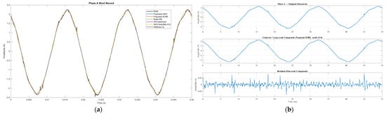
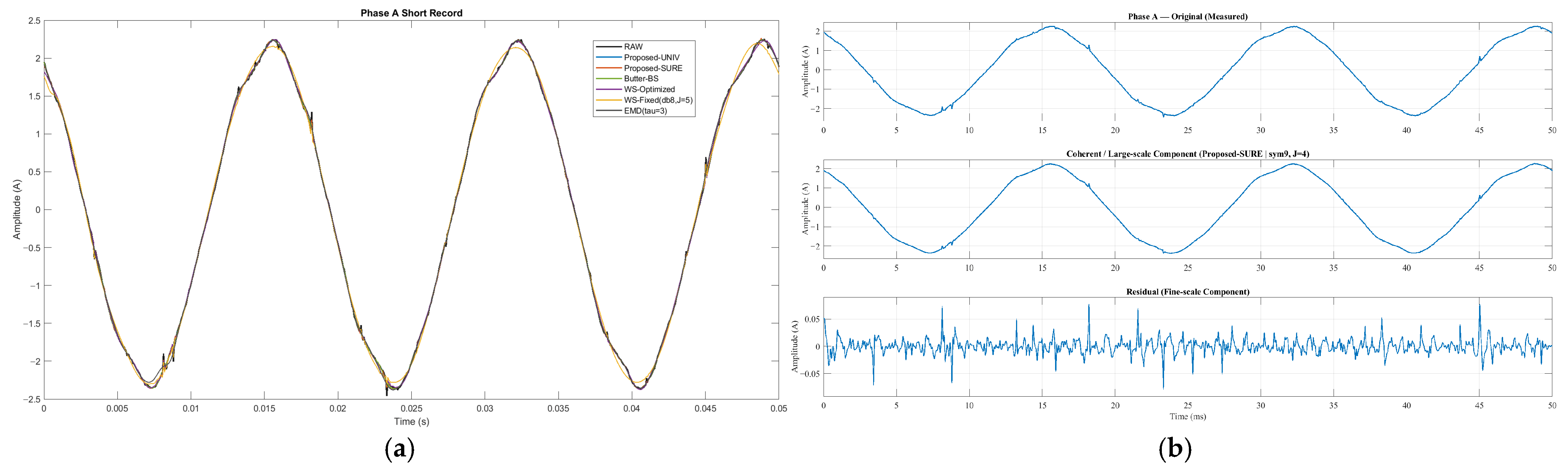
The time-domain comparison (Figure 5a) shows near-perfect overlap of the RAW, Proposed-UNIV, and Proposed-SURE waveforms across three cycles of Phase-A current, consistent with the expected sinusoidal response of a healthy motor under steady-state conditions. Figure 5b further illustrates the framework’s decomposition: the coherent component closely matches the measured signal, while the residual captures stochastic fluctuations removed during denoising. Its low broadband amplitude confirms suppression of random variations without altering harmonic structures, consistent with the steady operating condition of the Baldor motor.

Figure 5. Time-domain behavior of the proposed denoising framework for the short-signal record. (a) Comparison of the Phase-A current waveform under different denoising methods. (b) Multiresolution decomposition illustrating the original signal, the coherent large-scale component, and the residual disturbance-dominated component removed during denoising.

5.2. Long-Signal Analysis

To further evaluate the robustness of the proposed framework, a second experimental scenario was conducted using a long-duration current signal acquired from a U.S. Electrical Motors 215T induction motor operating under steady-state conditions. While the short-signal experiment provides a localized view of the denoising process, the extended scenario enables assessment of the temporal consistency of the method over prolonged observation intervals.

5.2.1. Optimal Wavelet Selection Across Windows

The optimal wavelet parameters for each analysis window are summarized in Table 5. The optimization consistently selects the Coiflet wavelet ($\mathrm{coif}2,\mathrm{J}=1$) with the same decomposition level, yielding scores close to unity across all windows.

Table 5. Optimal wavelet selection per analysis window.

Window	Samples	$\mathbf{Wavelet}(\psi$)	$\mathbf{J}$	Selection Score
1	1–6000	coif2	1	0.99991
2	6001–12,000	coif2	1	0.99990
3	12,001–18,000	coif2	1	0.99990
4	18,001–24,000	coif2	1	0.99990
5	24,001–30,000	coif2	1	0.99991

This stable selection indicates that the spectral characteristics of the stator current remain consistent throughout the long-duration signal and confirms that the proposed optimization strategy reliably identifies an appropriate multiresolution configuration.

5.2.2. Long-Signal Denoising Performance

The quantitative attenuation and spectral preservation metrics for representative analysis windows are reported in Table 6 and Table 7, revealing different attenuation–distortion trade-offs among the evaluated methods.

Table 6. Quantitative attenuation and spectral preservation metrics for the long-duration current signal (Window 1).

Method	NRR_att (dB)	$\mathbf{Energy}\mathbf{Attenuation}\mathbf{in}{\mathbf{B}}_{\mathbf{att}}$ (%)	$\mathbf{Mean}\mid \Delta \mid$ (dB)	$\mathbf{Max}\mid \Delta \mid$ (dB)	${\mathbf{RMSE}}_{\mathbf{PSD}}$ (dB)
Proposed-UNI	9.9251 × 10−11	2.2853 × 10−9	8.6673 × 10−11	1.2403 × 10−10	9.4809 × 10−11
Proposed-SURE	9.9251 × 10−11	2.2853 × 10−9	8.6673 × 10−11	1.2403 × 10−10	9.4809 × 10−11
Butterworth-BS	17.663	98.287	0.05693	0.97678	0.17627
WS-Optimized	2.4009	42.467	0.33035	3.283	0.64531
WS-Fixed	2.551	44.422	11.578	27.759	11.303
EMD	7.4495 × 10−11	1.7153 × 10−9	1.0486 × 10−7	4.8113 × 10−6	4.54 × 10−6

Table 7. Quantitative attenuation and spectral preservation metrics for the long-duration current signal (Window 3).

Method	NRR_att (dB)	$\mathbf{Energy}\mathbf{Attenuation}\mathbf{in}{\mathbf{B}}_{\mathbf{att}}$ (%)	$\mathbf{Mean}\mid \Delta \mid$ (dB)	$\mathbf{Max}\mid \Delta \mid$ (dB)	${\mathbf{RMSE}}_{\mathbf{PSD}}$ (dB)
Proposed-UNI	9.889 × 10−11	2.277 × 10−9	8.6778 × 10−11	1.2402 × 10−10	9.4808 × 10−11
Proposed-SURE	9.889 × 10−11	2.277 × 10−9	8.6778 × 10−11	1.2402 × 10−10	9.4808 × 10−11
Butterworth-BS	17.225	98.105	0.056487	0.91429	0.17616
WS-Optimized	2.4382	42.96	0.41555	3.8718	0.85816
WS-Fixed	3.0631	50.605	12.881	33.132	12.849
EMD	−5.9375 × 10−11	−1.3672 × 10−9	6.4146 × 10−8	3.7391 × 10−6	1.933 × 10−6

The Butterworth band-stop filter produces the largest energy reduction within the attenuation band ${\mathrm{B}}_{\mathrm{att}}$, with ${\mathrm{NRR}}_{\mathrm{att}}=17.663$ dB and $17.225\mathrm{d}$B for Windows 1 and 3, corresponding to energy attenuation percentages of 98.287% and 98.105%, respectively. However, this strong suppression is accompanied by measurable spectral distortion, with mean $\mid \Delta \mid$ values of 0.05693 dB and 0.056487 dB, maximum deviations approaching 0.98 dB, and ${\mathrm{RMSE}}_{\mathrm{PSD}}$ values around 0.176 dB, indicating modification of the spectral profile of the current signal.

In contrast, the proposed framework preserves the spectral structure with extremely high fidelity. For both threshold rules, mean $\mid \Delta \mid$ values remain on the order of ${10}^{-11}$ dB, the maximum deviations are approximately $1.24\times {10}^{-10}$ dB, and ${\mathrm{RMSE}}_{\mathrm{PSD}}$ is about $9.48\times {10}^{-11}$ dB in both windows. These values fall within numerical precision, indicating that the denoising process introduces no measurable spectral distortion. At the same time, attenuation indicators within ${\mathrm{B}}_{\mathrm{att}}$ remain close to zero, showing that under steady-state conditions, the framework operates conservatively and avoids modifying spectral components.

The wavelet shrinkage baselines exhibit substantially larger distortions. WS-Optimized produces mean $\mid \Delta \mid$ values between 0.33 dB and 0.42 dB, with maximum deviations exceeding 3.8 dB, whereas WS-Fixed introduces severe spectral alterations, with mean deviations above 11 dB and maximum deviations reaching 27–33 dB.

The EMD method preserves the spectral structure with very small deviations, with mean $\mid \Delta \mid$ values on the order of ${10}^{-7}$–${10}^{-8}$ dB and ${\mathrm{RMSE}}_{\mathrm{PSD}}$ around ${10}^{-6}$ dB. However, attenuation indicators within ${\mathrm{B}}_{\mathrm{att}}$ remain essentially null, indicating that the method does not produce measurable energy reduction in the evaluated band.

Overall, the results highlight distinct attenuation–distortion trade-offs: Butterworth achieves strong attenuation at the cost of spectral distortion; wavelet shrinkage produces increasingly large alterations; EMD preserves the spectrum but provides negligible attenuation; and the proposed framework maintains spectral structure within numerical precision while avoiding unnecessary modification of diagnostically relevant components.

5.2.3. Time-Frequency Behavior

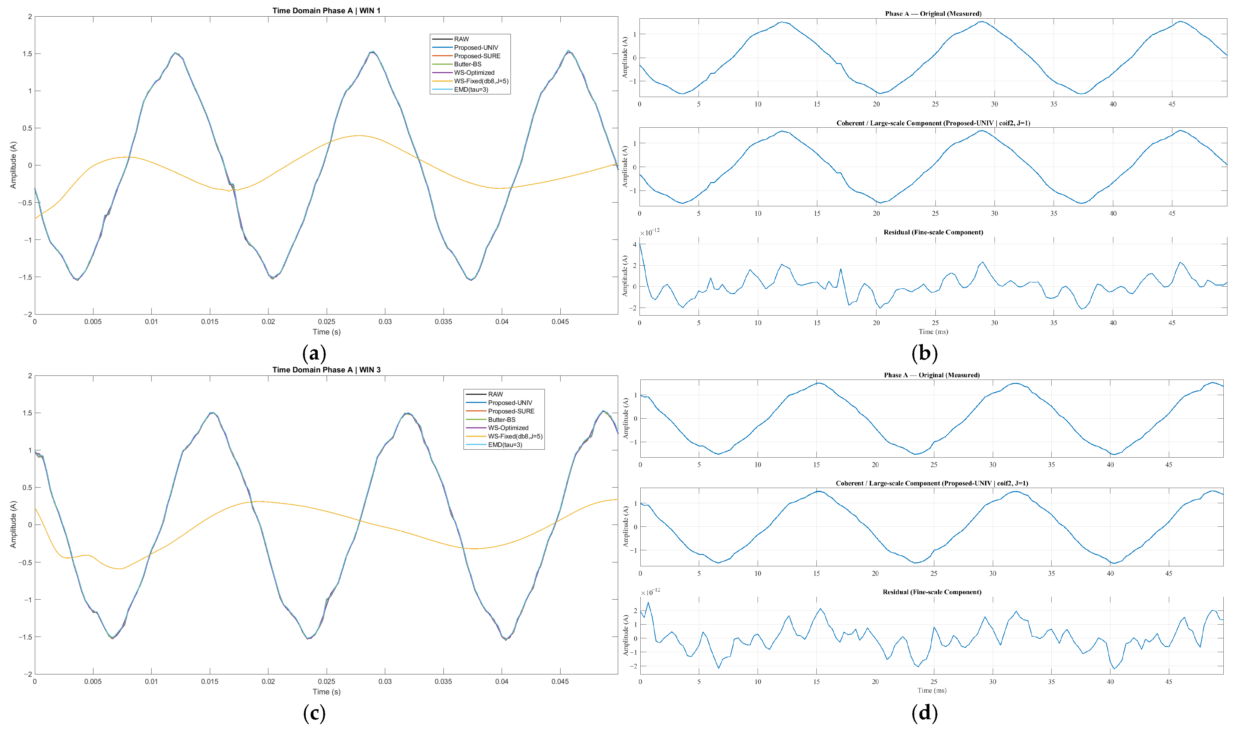
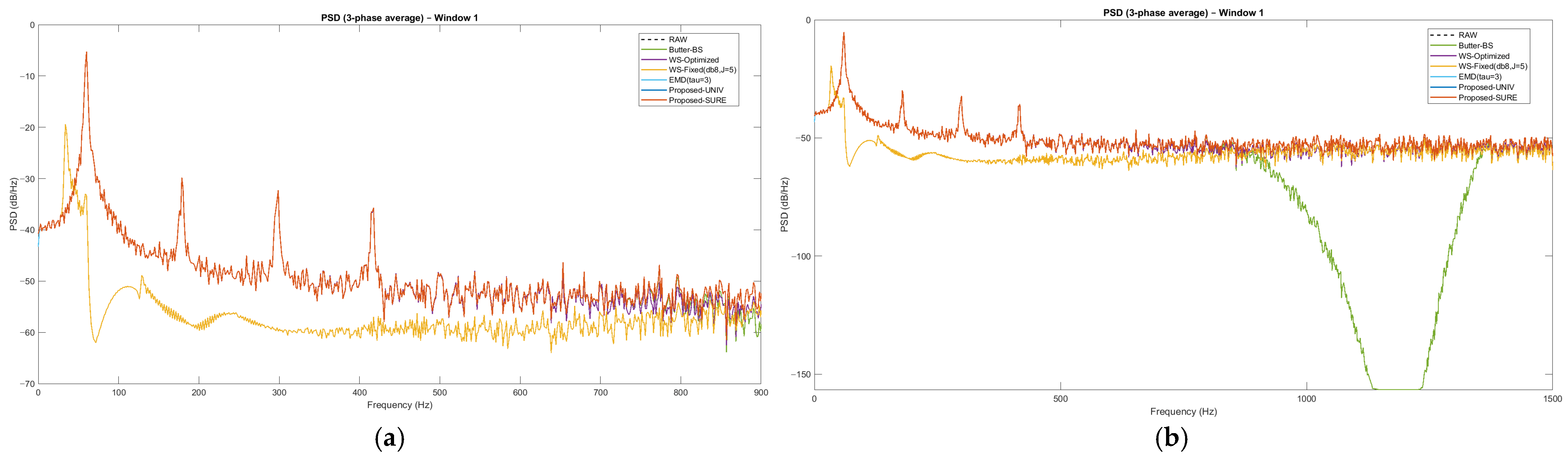
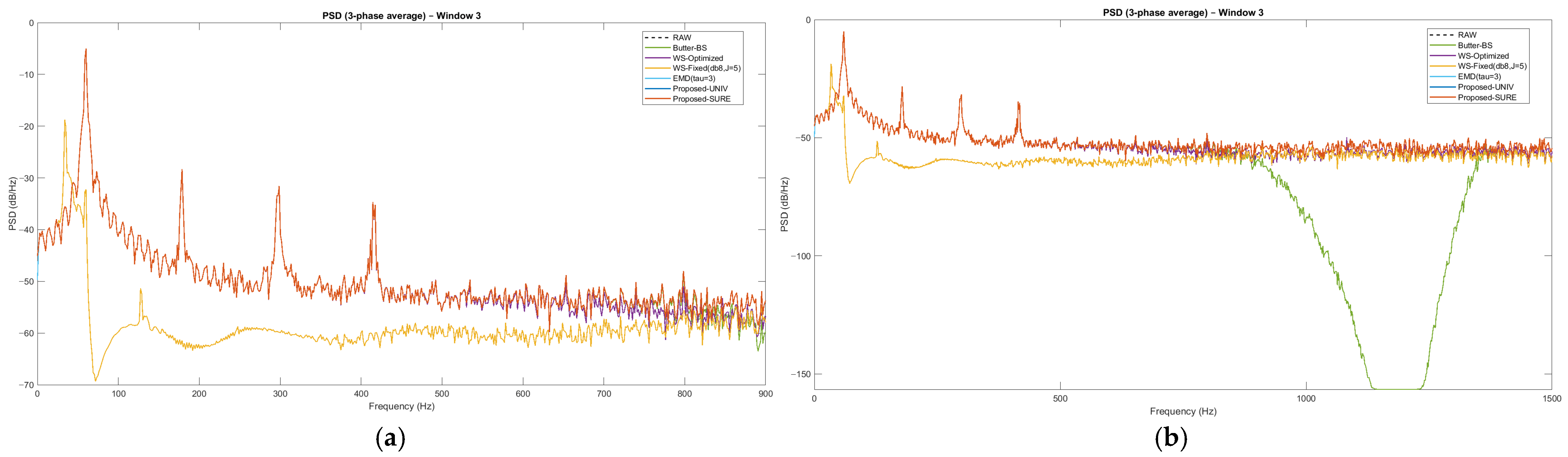
The temporal and spectral behavior of the proposed framework for representative analysis windows is illustrated in Figure 6, Figure 7 and Figure 8. In the time domain (Figure 6), the denoised signals obtained with the proposed framework remain practically indistinguishable from the RAW waveform for both analysis windows, confirming preservation of the stator current morphology. The multiresolution decomposition further clarifies this behavior: the coherent large-scale component closely reproduces the measured signal, while the residual isolates small-amplitude broadband fluctuations associated with disturbance-dominated fine-scale variations removed during denoising.

Figure 6. Time-domain behavior of the proposed denoising framework for representative analysis windows. (a) Phase-A current waveform comparison for Window 1 under different denoising methods. (b) Multiresolution decomposition for Window 1, showing the original signal, the coherent large-scale component, and the residual disturbance-dominated component removed during denoising. (c) Phase-A current waveform comparison for Window 3. (d) Multiresolution decomposition for Window 3.

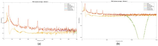
Figure 7. Power spectral density (PSD) analysis of the three-phase averaged stator current for Window 1. (a) Zoomed PSD in the protected harmonic region showing preservation of the fundamental component and higher-order harmonics after denoising. (b) Full-spectrum PSD highlighting the attenuation band and the notch introduced in the rejection region.

Figure 8. Power spectral density (PSD) analysis of the three-phase averaged stator current for Window 3. (a) Zoomed PSD in the protected harmonic region showing preservation of the fundamental component and higher-order harmonics after denoising. (b) Full-spectrum PSD highlighting the attenuation band and the notch introduced in the rejection region.

The spectral behavior is analyzed through the PSD representations shown in Figure 7 and Figure 8 for Windows 1 and 3, respectively. Each figure includes two complementary views: a zoomed PSD of the protected harmonic region (subfigure a) and the full-spectrum PSD (subfigure b).

For Window 1 (Figure 7a), the zoomed PSD shows that the proposed framework closely reproduces the RAW spectrum, preserving the fundamental component and higher-order harmonics with negligible deviation. This observation is consistent with the minimal spectral errors reported in Table 6 and Table 7. In contrast, the wavelet shrinkage baselines introduce visible distortions: WS-Optimized partially suppresses harmonic peaks, while WS-Fixed significantly alters the spectral envelope. The EMD method preserves the harmonic structure more faithfully but produces no noticeable attenuation in the evaluated band. The full-spectrum view (Figure 7b) highlights the strong attenuation notch introduced by the Butterworth band-stop filter within the predefined stopband, where spectral energy is almost completely removed.

A similar pattern is observed for Window 3 (Figure 8). The zoomed PSD (Figure 8a) again confirms that the proposed framework preserves the harmonic structure, maintaining a spectral envelope nearly identical to the RAW signal. In contrast, the wavelet shrinkage methods introduce broader distortions, particularly for WS-Fixed, while EMD maintains spectral shape but without measurable attenuation. The full-range PSD (Figure 8b) further emphasizes the pronounced attenuation notch produced by the Butterworth filter in the rejection band.

These results highlight a limitation of fixed filtering approaches: defining a cutoff frequency ${\mathrm{f}}_{\mathrm{c}}$ without prior knowledge of disturbance characteristics may remove diagnostically relevant spectral components. In motor condition monitoring, higher-order harmonics and modulation sidebands often contain information related to mechanical faults such as bearing defects or rotor asymmetries. If these components fall within the stopband, the filter suppresses them entirely. In contrast, the proposed framework preserves the harmonic structure of the stator current while isolating disturbance-driven fluctuations through multiresolution analysis, ensuring that the spectral information remains fully available for diagnostic interpretation.

5.2.4. Harmonic Component Preservation

To further assess spectral integrity, the deviations of the principal harmonic components and their associated sidebands were evaluated. Table 8 and Table 9 report the spectral deviations for ${\mathrm{H}}_1$, ${\mathrm{H}}_9$, ${\mathrm{H}}_{11}$, and ${\mathrm{H}}_{13}$ and their slip-related sidebands for analysis windows 1 and 3. The proposed framework preserves all evaluated components with negligible deviations, typically below ${10}^{-3}$ dB. In both windows, Proposed-UNIVERSAL and Proposed-SURE maintain deviations essentially equal to zero for the fundamental component and higher-order harmonics, including their associated sidebands.

Table 8. Spectral deviations of harmonic and sideband components after denoising (Window 1).

Spectral Component	${\mathbf{f}}_0\left(\mathbf{Hz}\right)$	$\mathbf{Raw}\text{\_}\mathbf{dB}$	$\Delta \mathbf{Proposed}$ $\mathbf{UNIVERSAL}$ (dB)	Δ Proposed SURE (dB)	Δ Butter (dB)	Δ WS-Opt (dB)	Δ WS-Fix (dB)	Δ EMD (dB)
${\mathrm{H}}_1$	60.06	−5.229	−0.000	0.000	−0.000	−0.000	−27.759	−0.000
${\mathrm{H}}_1-{\mathrm{f}}_{\mathrm{r}}$	26.37	−36.590	−0.000	0.000	−0.000	−0.000	10.051	0.005
${\mathrm{H}}_1+{\mathrm{f}}_{\mathrm{r}}$	93.75	−34.811	−0.000	0.000	−0.001	0.018	−17.001	−0.000
${\mathrm{H}}_1-{2\mathrm{sf}}_s$	55.94	−5.229	−0.000	0.000	−0.000	−0.000	−27.759	−0.000
${\mathrm{H}}_1+{2\mathrm{sf}}_{\mathrm{s}}$	64.18	−5.229	−0.000	0.000	−0.000	−0.000	−27.759	−0.000
${\mathrm{H}}_9$	540.53	−48.139	−0.000	−0.000	−0.004	0.151	−8.723	0.000
${\mathrm{H}}_9-{\mathrm{f}}_{\mathrm{r}}$	506.84	−48.532	−0.000	−0.000	−0.002	−0.186	−8.821	−0.000
${\mathrm{H}}_9+{\mathrm{f}}_{\mathrm{r}}$	574.22	−50.684	−0.000	−0.000	−0.008	0.217	−6.623	−0.000
${\mathrm{H}}_9-{2\mathrm{sf}}_s$	536.41	−50.032	−0.000	−0.000	−0.003	0.057	−7.932	0.000
${\mathrm{H}}_9+{2\mathrm{sf}}_s$	544.64	−48.139	−0.000	−0.000	−0.004	0.151	−8.723	0.000
${\mathrm{H}}_{11}$	660.64	−51.477	−0.000	−0.000	−0.045	−0.260	−6.334	−0.000
${\mathrm{H}}_{11}-{\mathrm{f}}_{\mathrm{r}}$	626.95	−49.486	−0.000	−0.000	−0.021	−0.385	−6.229	−0.000
${\mathrm{H}}_{11}+{\mathrm{f}}_{\mathrm{r}}$	694.34	−49.989	−0.000	−0.000	−0.087	−0.509	−5.967	0.000
${\mathrm{H}}_{11}-{2\mathrm{sf}}_s$	656.53	−46.331	−0.000	−0.000	−0.035	−2.631	−11.480	−0.000
${\mathrm{H}}_{11}+{2\mathrm{sf}}_s$	664.76	−51.477	−0.000	−0.000	−0.045	0.039	−3.368	−0.000
${\mathrm{H}}_{13}$	780.76	−49.344	−0.000	−0.000	−0.428	−1.345	−6.285	−0.000
${\mathrm{H}}_{13}-{\mathrm{f}}_{\mathrm{r}}$	747.07	−50.343	−0.000	−0.000	−0.232	−1.325	−5.668	0.000
${\mathrm{H}}_{13}+{\mathrm{f}}_{\mathrm{r}}$	814.45	−51.407	−0.000	−0.000	−0.977	−1.147	−4.372	0.003
${\mathrm{H}}_{13}-{2\mathrm{sf}}_s$	776.64	−46.840	−0.000	−0.000	−0.402	−3.283	−8.271	−0.000
${\mathrm{H}}_{13}+{2\mathrm{sf}}_s$	784.88	−51.448	−0.000	−0.000	−0.570	−2.354	−5.410	0.006

Table 9. Spectral deviations of harmonic and sideband components after denoising (Window 3).

Spectral Component	${\mathbf{f}}_0\left(\mathbf{Hz}\right)$	$\mathbf{Raw}\text{\_}\mathbf{dB}$	$\Delta \mathbf{Proposed}$ $\mathbf{UNIVERSAL}$ (dB)	Δ Proposed SURE (dB)	Δ Butter (dB)	Δ WS-Opt (dB)	Δ WS-Fix (dB)	Δ EMD (dB)
${\mathrm{H}}_1$	60.06	−4.995	−0.000	0.000	0.000	0.000	−27.194	−0.000
${\mathrm{H}}_1-{\mathrm{f}}_{\mathrm{r}}$	26.37	−36.600	−0.000	0.000	0.001	−0.000	6.987	−0.004
${\mathrm{H}}_1+{\mathrm{f}}_{\mathrm{r}}$	93.75	−36.366	−0.000	0.000	0.001	0.000	−23.477	−0.000
${\mathrm{H}}_1-{2\mathrm{sf}}_s$	55.94	−4.995	−0.000	0.000	0.000	0.000	−27.194	−0.000
${\mathrm{H}}_1+{2\mathrm{sf}}_{\mathrm{s}}$	64.18	−4.995	−0.000	0.000	0.000	0.000	−27.194	−0.000
${\mathrm{H}}_9$	540.53	−49.683	−0.000	−0.000	−0.003	−1.021	−9.126	0.000
${\mathrm{H}}_9-{\mathrm{f}}_{\mathrm{r}}$	506.84	−51.940	−0.000	−0.000	−0.002	0.001	−6.205	−0.000
${\mathrm{H}}_9+{\mathrm{f}}_{\mathrm{r}}$	574.22	−51.289	−0.000	−0.000	−0.008	−0.010	−6.737	0.000
${\mathrm{H}}_9-{2\mathrm{sf}}_s$	536.41	−49.683	−0.000	−0.000	−0.003	−1.021	−9.126	0.000
${\mathrm{H}}_9+{2\mathrm{sf}}_s$	544.64	−52.856	−0.000	−0.000	−0.004	−0.128	−5.952	−0.000
${\mathrm{H}}_{11}$	660.64	−52.829	−0.000	−0.000	−0.036	−1.021	−5.754	0.000
${\mathrm{H}}_{11}-{\mathrm{f}}_{\mathrm{r}}$	626.95	−50.900	−0.000	−0.000	−0.018	0.001	−7.786	0.000
${\mathrm{H}}_{11}+{\mathrm{f}}_{\mathrm{r}}$	694.34	−51.028	−0.000	−0.000	−0.079	−0.010	−6.183	0.000
${\mathrm{H}}_{11}-{2\mathrm{sf}}_s$	656.53	−48.804	−0.000	−0.000	−0.035	−1.021	−9.779	−0.000
${\mathrm{H}}_{11}+{2\mathrm{sf}}_s$	664.76	−51.591	−0.000	−0.000	−0.048	−0.128	−6.612	0.000
${\mathrm{H}}_{13}$	780.76	−52.843	−0.000	−0.000	−0.518	−1.406	−4.720	0.000
${\mathrm{H}}_{13}-{\mathrm{f}}_{\mathrm{r}}$	747.07	−53.177	−0.000	−0.000	−0.247	−0.382	−4.271	−0.000
${\mathrm{H}}_{13}+{\mathrm{f}}_{\mathrm{r}}$	814.45	−51.580	−0.000	−0.000	−0.914	−2.832	−4.063	−0.000
${\mathrm{H}}_{13}-{2\mathrm{sf}}_s$	776.64	−50.377	−0.000	−0.000	−0.394	−3.872	−7.186	−0.000
${\mathrm{H}}_{13}+{2\mathrm{sf}}_s$	784.88	−52.843	−0.000	−0.000	−0.518	−2.560	−4.720	0.000

In contrast, the baseline methods introduce larger spectral alterations. The Butterworth band-stop filter produces moderate distortions, reaching deviations of about −0.98 dB for ${\mathrm{H}}_{13}+{\mathrm{f}}_{\mathrm{r}}$ component. The wavelet shrinkage baselines show stronger effects: WS-Optimized introduces deviations up to −3.87 dB; while WS-Fixed yields the largest distortions, reaching −27.7 dB for components around the fundamental and −23.5 dB for sidebands in Window 3. The EMD method also preserves harmonic amplitudes with small deviations; however, as shown in Table 6 and Table 7, this occurs with almost no disturbance attenuation.

Overall, the proposed framework preserves the harmonic structure—including the fundamental, higher-order harmonics, and their sidebands—with negligible deviations, while baseline methods introduce progressively larger distortions. This capability ensures spectral fidelity and supports reliable motor condition monitoring.

6. Conclusions

This paper presented a physically constrained wavelet-based denoising framework for three-phase induction motor current signals, designed to suppress disturbance-dominated components while preserving diagnostically meaningful spectral information. Experimental results obtained from real three-phase stator current measurements under steady-state operating conditions show that the proposed method achieves noise reduction ratios on the order of 8–10 dB while maintaining spectral deviations of the main harmonic components below ${10}^{-3}$ dB, effectively within numerical precision. These results indicate that the denoising process removes disturbance-dominated fluctuations without altering the deterministic spectral structure of the current signal.

A key contribution of this work is the formulation of denoising as a physically constrained optimization problem, where wavelet parameters are selected through a multi-criteria objective function that jointly maximizes disturbance attenuation while preserving harmonic amplitudes, sideband structures, inter-phase coherence, and time-domain waveform integrity. This formulation enables both global optimization for short-duration signals and adaptive window-wise optimization for long-duration recordings, allowing the framework to operate consistently across segmented analysis intervals.

Comparative analysis with conventional baselines further highlights the advantages of the proposed approach. While the Butterworth band-stop filter achieves strong attenuation within predefined rejection bands, it introduces spectral distortions that propagate to neighboring components. The wavelet shrinkage baselines exhibit even larger alterations: WS-Optimized produces deviations of several decibels, while WS-Fixed introduces distortions exceeding 20–30 dB in several harmonic components, effectively suppressing parts of the harmonic structure. The EMD approach preserves harmonic amplitudes more faithfully but provides almost no disturbance attenuation, leaving disturbance energy essentially unchanged. In contrast, the proposed framework consistently preserves the harmonic components ${\mathrm{H}}_1$, ${\mathrm{H}}_9$, ${\mathrm{H}}_{11}$, and ${\mathrm{H}}_{13}$, together with their slip-related sidebands, across different analysis windows.

It is important to emphasize that the present study focuses exclusively on steady-state operating conditions and, therefore, does not include experiments under varying load conditions or mechanical fault scenarios. Such operating regimes introduce additional spectral dynamics that require dedicated investigation and will be addressed in future work. Consequently, the objective of this study is not to perform fault diagnosis directly, but to establish a physically consistent preprocessing framework capable of preserving diagnostically relevant spectral information prior to advanced condition monitoring algorithms.

Overall, the results indicate that the proposed approach provides a robust and physically grounded preprocessing stage for stator current analysis, particularly suitable for segmented analysis, short-duration measurements, and long-duration recordings requiring adaptive processing. Thus, the framework establishes a reliable foundation for current-based diagnostics in electrical machines and paves the way for future wavelet-based fault diagnosis methodologies.

References

- Sengamalai, U.; Anbazhagan, G.; Thamizh Thentral, T.M.; Vishnuram, P.; Khurshaid, T.; Kamel, S. Three Phase Induction Motor Drive: A Systematic Review on Dynamic Modeling, Parameter Estimation, and Control Schemes. Energies 2022, 15, 8260. [Google Scholar] [CrossRef] [Scilit]
- Abdo, A.; Siam, J.; Abdou, A.; Shehadeh, H.; Mustafa, R. Practical Test on the Operation of the Three-Phase Induction Motor under Single-Phasing Fault. Appl. Sci. 2024, 14, 4690. [Google Scholar] [CrossRef] [Scilit]
- AlShorman, O.; Irfan, M.; Abdelrahman, R.B.; Masadeh, M.; Alshorman, A.; Sheikh, M.A.; Saad, N.; Rahman, S. Advancements in Condition Monitoring and Fault Diagnosis of Rotating Machinery: A Comprehensive Review of Image-Based Intelligent Techniques for Induction Motors. Eng. Appl. Artif. Intell. 2024, 130, 107724. [Google Scholar] [CrossRef] [Scilit]
- Hamani, K.; Kuchar, M.; Kubatko, M.; Kirschner, S. Advancements in Induction Motor Fault Diagnosis and Condition Monitoring: A Comprehensive Review. Sensors 2025, 25, 5942. [Google Scholar] [CrossRef] [Scilit]
- Sobhi, S.; Reshadi, M.H.; Zarft, N.; Terheide, A.; Dick, S. Condition Monitoring and Fault Detection in Small Induction Motors Using Machine Learning Algorithms. Information 2023, 14, 329. [Google Scholar] [CrossRef] [Scilit]
- Nandi, S.; Toliyat, H.A. Condition Monitoring and Fault Diagnosis of Electrical Machines—A Review. In Conference Record—IAS Annual Meeting; IEEE Industry Applications Society: Piscataway, NJ, USA, 1999; Volume 1, pp. 197–204. [Google Scholar] [CrossRef] [Scilit]
- Li, Y.; Li, B.; Noman, K.; Wang, T.; Diversi, R.; Lenzi, A.; Speciale, N.; Barbieri, M. An Autoregressive-Based Motor Current Signature Analysis Approach for Fault Diagnosis of Electric Motor-Driven Mechanisms. Sensors 2025, 25, 1130. [Google Scholar] [CrossRef] [Scilit]
- Areias, I.A.D.S.; Da Silva, L.E.B.; Bonaldi, E.L.; De Oliveira, L.E.D.L.; Lambert-Torres, G.; Bernardes, V.A. Evaluation of Current Signature in Bearing Defects by Envelope Analysis of the Vibration in Induction Motors. Energies 2019, 12, 4029. [Google Scholar] [CrossRef] [Scilit]
- Bhole, N.; Ghodke, S.S. Motor Current Signature Analysis for Fault Detection of Induction Machine—A Review. In Proceedings of the 2021 International Conference on Nascent Technologies in Engineering, ICNET 2021, Virtual, 15–16 January 2021. [Google Scholar] [CrossRef] [Scilit]
- Liu, D.; Inoue, H.; Kanemaru, M. Robust Motor Current Signature Analysis (MCSA)-Based Fault Detection under Varying Operating Conditions. In Proceedings of the 2022 International Conference on Electrical Machines and Systems, ICEMS 2022, Chiang Mai, Thailand, 29 November–2 December 2022. [Google Scholar] [CrossRef] [Scilit]
- Thomson, W.T.; Culbert, I. Current Signature Analysis for Condition Monitoring of Cage Induction Motors: Industrial Application and Case Histories; Wiley: Hoboken, NJ, USA, 2016; pp. 1–397. [Google Scholar] [CrossRef] [Scilit]
- Benbouzid, M.E.H. A Review of Induction Motors Signature Analysis as a Medium for Faults Detection. IEEE Trans. Ind. Electron. 2000, 47, 984–993. [Google Scholar] [CrossRef] [Scilit]
- Bellini, A.; Filippetti, F.; Tassoni, C.; Capolino, G.A. Advances in Diagnostic Techniques for Induction Machines. IEEE Trans. Ind. Electron. 2008, 55, 4109–4126. [Google Scholar] [CrossRef] [Scilit]
- Henao, H.; Capolino, G.A.; Fernandez-Cabanas, M.; Filippetti, F.; Bruzzese, C.; Strangas, E.; Pusca, R.; Estima, J.; Riera-Guasp, M.; Hedayati-Kia, S. Trends in Fault Diagnosis for Electrical Machines: A Review of Diagnostic Techniques. IEEE Ind. Electron. Mag. 2014, 8, 31–42. [Google Scholar] [CrossRef] [Scilit]
- Gonzalez, P.; Buigues, G.; Mazon, A.J. Noise in Electric Motors: A Comprehensive Review. Energies 2023, 16, 5311. [Google Scholar] [CrossRef] [Scilit]
- Wang, Z.; Gu, Y.; Chen, C.; Wang, L.; Sun, X. Induction Motor Noise Source Separation and Identification Based on Adaptive Scale-Space Mode Extraction. Machines 2023, 11, 449. [Google Scholar] [CrossRef] [Scilit]
- Xu, K.; Song, X. A Current Noise Cancellation Method Based on Fractional Linear Prediction for Bearing Fault Detection. Sensors 2023, 24, 52. [Google Scholar] [CrossRef] [Scilit] [PubMed]
- Jaros, R.; Byrtus, R.; Dohnal, J.; Danys, L.; Baros, J.; Koziorek, J.; Zmij, P.; Martinek, R. Advanced Signal Processing Methods for Condition Monitoring. Arch. Comput. Methods Eng. 2022, 30, 1553–1577. [Google Scholar] [CrossRef] [Scilit]
- Jarosz, J.J.; Skowron, M.; Frankiewicz, O.; Wolkiewicz, M.; Weisse, S.; Valire, J.; Szabat, K. Diagnostic Signal Acquisition Time Reduction Technique in the Induction Motor Fault Detection and Localization Based on SOM-CNN. Electronics 2025, 14, 2373. [Google Scholar] [CrossRef] [Scilit]
- Thomas, K.; Rahman, A.; Rohouma, W.; Ahamed, M.F.; Shafi, F.B.; Nahiduzzaman, M.; Khandakar, A. Comprehensive Fault Diagnosis of Three-Phase Induction Motors Using Synchronized Multi-Sensor Data Collection. Sci. Data 2025, 12, 1468. [Google Scholar] [CrossRef] [Scilit]
- Yang, T.; Chen, X.; Liu, Y.; Luo, L.; Wang, Y.; Miao, Y.; Bin, S. Research on Electromagnetic Noise Suppression Methods for Vehicle-Mounted Induction Motors. Energies 2025, 18, 5430. [Google Scholar] [CrossRef] [Scilit]
- Giaouris, D.; Finch, J.W. Denoising Using Wavelets on Electric Drive Applications. Electr. Power Syst. Res. 2008, 78, 559–565. [Google Scholar] [CrossRef] [Scilit]
- Antoni, J. Fast Computation of the Kurtogram for the Detection of Transient Faults. Mech. Syst. Signal Process. 2007, 21, 108–124. [Google Scholar] [CrossRef] [Scilit]
- Mallat, S.G. A Theory for Multiresolution Signal Decomposition: The Wavelet Representation. IEEE Trans. Pattern Anal. Mach. Intell. 1989, 11, 674–693. [Google Scholar] [CrossRef] [Scilit]
- Mallat, S. A Wavelet Tour of Signal Processing: The Sparse Way; Academic Press: Cambridge, MA, USA, 2008; pp. 1–805. [Google Scholar] [CrossRef] [Scilit]
- Carrera-Avendaño, E.; Urquiza-Beltrán, G.; Trutié-Carrero, E.; Nieto-Jalil, J.M.; Carrillo-Pereyra, C.; Seuret-Jiménez, D. Detection of Crankshaft Faults by Means of a Modified Welch-Bartlett Periodogram. Eng. Fail. Anal. 2022, 132, 105938. [Google Scholar] [CrossRef] [Scilit]
- Yang, L.; Feng, F. Wavelet-Based Denoising Strategies for Non-Stationary Signals in Electrical Power Systems: An Optimization Perspective. Electronics 2025, 14, 3190. [Google Scholar] [CrossRef] [Scilit]
- Yan, Y.; Liu, Q.; Gao, X.Q. Motor Fault Diagnosis Algorithm Based on Wavelet and Attention Mechanism. J. Sens. 2021, 2021, 3782446. [Google Scholar] [CrossRef] [Scilit]
- Goh, Y.J.; Kim, K.M. Clarke-Park Transformation-Based Input Configuration for CNN Diagnosis of Stator Faults in Three Phase Induction Motors Using Motor Current Signature Analysis. IEEE Access 2025, 13, 150505–150516. [Google Scholar] [CrossRef] [Scilit]
- Krause, P.; Wasynczuk, O.; Sudhoff, S.; Pekarek, S. Analysis of Electric Machinery and Drive Systems; Wiley: Hoboken, NJ, USA, 2013. [Google Scholar] [CrossRef] [Scilit]
- O’Rourke, C.J.; Qasim, M.M.; Overlin, M.R.; Kirtley, J.L. A Geometric Interpretation of Reference Frames and Transformations: Dq0, Clarke, and Park. IEEE Trans. Energy Convers. 2019, 34, 2070–2083. [Google Scholar] [CrossRef] [Scilit]
- Clarke, E. Circuit Analysis of A-C Power Systems; Wiley: Hoboken, NJ, USA, 1943. [Google Scholar]
- Daubechies, I. Ten Lectures on Wavelets; Society for Industrial and Applied Mathematics (SIAM): Philadelphia, PA, USA, 1992. [Google Scholar] [CrossRef] [Scilit]
- Christensen, O. An Introduction to Frames and Riesz Bases; Springer Nature: Durham, NC, USA, 2016. [Google Scholar] [CrossRef] [Scilit]
- Welch, P.D. The Use of Fast Fourier Transform for the Estimation of Power Spectra: A Method Based on Time Averaging Over Short, Modified Periodograms. IEEE Trans. Audio Electroacoust. 1967, 15, 70–73. [Google Scholar] [CrossRef] [Scilit]
- Kunjir, R.; Bhanuse, V.; Kulkarni, J.; Patankar, S. Determination of Deformation of Steel Plate Using Welch’s Periodogram Estimate. In Proceedings of the 2nd International Conference on Intelligent Computing and Control Systems, ICICCS 2018; IEEE: New York, NY, USA, 2019; pp. 1169–1174. [Google Scholar]
- Donoho, D.L. De-Noising by Soft-Thresholding. IEEE Trans. Inf. Theory 1995, 41, 613–627. [Google Scholar] [CrossRef] [Scilit]
- Donoho, D.L.; Johnstone, J.M. Ideal Spatial Adaptation by Wavelet Shrinkage. Biometrika 1994, 81, 425–455. [Google Scholar] [CrossRef]
- Antoniou, A. DIGITAL FILTERS: ANALYSIS AND DESIGN; McGraw-Hill: Columbus, UH, USA, 1993. [Google Scholar]
- Zhang, X.; Iwakura, H. Design of IIR Digital Filters Based on Eigenvalue Problem. IEEE Transactions on Signal Processing 1996, 44, 1325–1333. [Google Scholar] [CrossRef] [Scilit]
- Davis, D.J.; Challis, J.H. Automatic Segment Filtering Procedure for Processing Non-Stationary Signals. J. Biomech. 2020, 101, 109619. [Google Scholar] [CrossRef] [Scilit] [PubMed]
- Minoshima, S.; Maruno, H.; Yui, N.; Togawa, T.; Kinoshita, F.; Kubota, M.; Berger, K.L.; Uchida, Y.; Uno, K.; Arimizu, N. Optimization of Butterworth Filter for Brain SPECT Imaging. Ann. Nucl. Med. 1993, 7, 71–77. [Google Scholar] [CrossRef] [Scilit] [PubMed]
- Huang, N.E.; Shen, Z.; Long, S.R.; Wu, M.C.; Snin, H.H.; Zheng, Q.; Yen, N.C.; Tung, C.C.; Liu, H.H. The Empirical Mode Decomposition and the Hilbert Spectrum for Nonlinear and Non-Stationary Time Series Analysis. Proc. R. Soc. A Math. Phys. Eng. Sci. 1998, 454, 903–995. [Google Scholar] [CrossRef] [Scilit]
- Mohguen, W.; Bekka, R.E.H. EMD-Based Denoising by Customized Thresholding. In Proceedings of the 2017 International Conference on Control, Automation and Diagnosis, ICCAD 2017, Hammamet, Tunisia, 19–21 January 2017; pp. 19–23. [Google Scholar] [CrossRef] [Scilit]
- INA114 Data Sheet, Product Information and Support|TI.Com. Available online: https://www.ti.com/product/INA114 (accessed on 1 February 2026).
Disclaimer/Publisher’s Note: The statements, opinions and data contained in all publications are solely those of the individual author(s) and contributor(s) and not of MDPI and/or the editor(s). MDPI and/or the editor(s) disclaim responsibility for any injury to people or property resulting from any ideas, methods, instructions or products referred to in the content. |
© 2026 by the authors. Licensee MDPI, Basel, Switzerland. This article is an open access article distributed under the terms and conditions of the Creative Commons Attribution (CC BY) license.