Investment Deficit Measurement of Flexible Generation for Consuming Renewables

Abstract

Integrating renewable energy into power grids is critical for advancing low-carbon transitions. However, the inherent variability of renewables requires flexible generation resources—predominantly thermal power units—to maintain real-time grid balancing. Although these flexible generators earn revenue from electricity production, they often incur significant deficits in recovering their upfront investment and retrofitting costs. While existing research has largely focused on short-term balancing expenses, this persistent investment gap remains underexplored. This article analyzes the causes of the investment deficit in the flexible generation assets needed to support renewable integration. To more comprehensively assess system integration costs, we propose a modeling framework that quantifies the investment and construction costs incurred due to renewable volatility. Through simulation, we estimate the required flexible capacity, associated costs, and operational revenues, thereby calculating the investment gap directly attributable to renewable integration. The model feasibility is further verified via sensitivity analysis. Additionally, the study outlines a conceptual cost allocation mechanism and demonstrates how the proposed method can be extended to assess other types of grid-supporting resources. These insights contribute to improved electricity market design, support evidence-based energy policymaking, and facilitate the market-oriented reform of the power sector.

1. Introduction

In order to solve the energy shortage and greenhouse effect, more and more countries are encouraged to reduce the share of fossil fuels in their energy systems, and strengthen the development and utilization of renewable energy such as wind energy, photovoltaics, and tidal energy [1,2,3]. Today’s world is committed to accelerating the development of renewable energy to achieve carbon emission standards [4,5]. Currently, wind power accounts for approximately 37% of Ireland’s electricity supply [5]. By 2050, Ireland’s installed onshore wind power capacity is expected to expand from 4.3 GW to 11–16 GW, and offshore wind power is expected to reach 30 GW [6]. Since the carbon peak and carbon neutrality goals were proposed in 2020, China’s renewable energy has also developed rapidly. As of the end of 2021, China’s cumulative non-fossil energy installed capacity reached 1120 GW, accounting for 47% of the total installed capacity, exceeding the coal power installed capacity for the first time. The installed capacity of wind power and photovoltaics both exceeds 300 GW, and the proportion of related power generation in total power generation exceeds 10% for the first time [7,8]. It is expected that China’s renewable energy will maintain its rapid growth by 2030 [9]. However, due to the high uncertainty and unpredictability of renewable energy, the volatility and prediction error of renewable energy power generation are relatively large, and it cannot be directly connected to the grid. Therefore, the power system needs to be renovated to match these characteristics, so that it can be safely, stably, and efficiently utilized. This is the consumption of renewables. During the process of consumption, additional costs are inevitably incurred, including the balancing cost of providing balanced services for renewable energy and the investment and construction cost of power grid construction and transformation. The construction of supporting power sources is one of the projects of power grid transformation. Traditional thermal power units have the characteristics of stable output and large inertia, which can effectively cope with the fluctuations of renewables and facilitate their smooth grid connection [10]. Its construction will inevitably incur certain costs. Therefore, this paper mainly studies the construction costs of supporting power sources during the process of renewables grid connection.

Currently, there are many studies on the cost of renewables’ consumption. Envelope et al. conducted a systematic analysis of the driving factors of balance cost, proposed a modeling method of balance cost, and looked forward to the potential development trend of balance cost [11]. Liu et al. scientifically calculated the balance cost and promoted the reasonable distribution of benefits between renewables and conventional energy [12]. Singh et al. conducted a balance cost analysis on a hybrid system containing wind power, photovoltaic, energy storage, and traditional power sources. The core goal was to optimize the total power generation cost by minimizing the balance cost of the wind energy hybrid system [13]. Liu et al. built a mathematical prediction model, combined with a load credible capacity and an adjustable potential prediction model based on response reliability indicators and confidence intervals, to quantitatively calculate the power balance gap. At the same time, the priority method was used to evaluate the system balance cost scale [12]. Dai et al. evaluated the power purchase cost and grid connection costs of developing grid-connected renewable energy in China, and analyzed its sharing mechanism among different stakeholders, aiming to quantify the additional system costs caused by the frequent adjustments of traditional power plants forced by fluctuations in wind power output [14]. Envelope et al. studied and quantified the indirect costs of coal power unit operation caused by integrating renewable energy into the grid [10]. Gianfreda et al. explored the impact of market design on balancing costs and emphasized the importance of improving market mechanisms and strengthening supervision [15]. G et al. explored the impact of flexible resources such as conventional power generation, energy storage, and demand-side response on balance costs [16]. Existing research has made certain progress in exploring the influencing factors of the balance cost of renewables, establishing models for the balance cost of renewables, and optimizing related models. And, on this basis, some scholars have conducted research on the cost-sharing mechanism for balancing renewables. However, most of the existing studies are about balancing costs, and there are few studies on the investment and construction costs generated by power grid renovations. The calculation of the investment and construction costs of renewables is conducive to a more scientific and comprehensive assessment of the consumption costs of renewables, which serves as the foundation for the subsequent allocation work and the formulation of the power market mechanism. To fill the gap in this field, to calculate the consumption cost of renewables more comprehensively, and, at the same time, to lay the foundation for subsequent allocation, this paper presents a brand-new approach to quantifying the investment and construction costs of supporting power sources in the cost of renewables’ consumption. The main function of the flexible generation for renewables is to balance the volatility of renewables’ power generation. During its construction process, construction and renovation costs will be incurred. During operation, the newly added units will also generate electricity and bring certain profits. We believe that this part of the revenue can compensate for certain speculative construction costs. Therefore, the difference between the investment and construction cost of the supporting power source and the power generation revenue of the newly added units is regarded as the consumption cost of the supporting power source that the renewables should bear during the power generation process. To reflect the volatility of renewables and ensure the reliability of the system, we obtained the investment and construction costs of the newly added supporting power sources, and the revenue of the newly added generating units, by comparing the two extreme ideal situations of the output of renewables based on the trusted capacity and the output based on the installed capacity, and then obtained the investment cost difference in the supporting power sources. The results show that the investment deficit of flexible generation for consuming renewables is relatively large and cannot be ignored. It is necessary to take it into account in the consumption cost of renewables. This method can provide certain references for the subsequent design of the apportionment mechanism, thereby further improving the market mechanism. It is conducive to decision makers designing energy policies and promoting the market-oriented reform of the power industry. The main contents are as follows:

• The reasons for the investment cost gap in renewables’ flexible generation are analyzed, and, based on this, a framework for the investment deficit of flexible generation for consuming of renewables is constructed.
• A model to measure the investment deficit of flexible generation for consuming of renewables was built, including a power planning model, an economic dispatch model, and an investment deficit calculation model of flexible generation for the consumption of renewables.
• The IEEE system was used to calculate the investment deficit of flexible generation for the consumption of renewables.

2. Materials and Methods

2.1. Investment Gap for Flexible Generation for Renewables

2.1.1. Analysis of the Investment Gap for Flexible Generation for Renewables

Traditional coal power and nuclear power can generate electricity according to instructions when needed. However, for renewables, such as wind power and photovoltaic, their power generation is volatile, intermittent, and uncertain. The installed capacity of renewables is not equal to its effective capacity to provide power support for the grid at critical moments (such as the evening when electricity consumption peaks in summer). Therefore, the concept of renewables’ credible capacity (Credible Capacity) is proposed. Renewable energy credible capacity refers to the proportion of capacity that is equivalent to conventional power generation serving renewables loads at the same reliability level. To ensure the safe operation of the power system after renewables are connected to the grid, its credible capacity must be considered [17]. Assuming that renewable sources are based on the installed capacity, flexible generation supplies at this time are planned under a completely ideal state. However, in the actual production process, we must fully consider the reliability of renewables’ output. Therefore, the flexible generation must be planned under the condition that credible capacity is used as a renewable output. Generally, the planned power supply capacity under actual production conditions will exceed the planned power supply unit capacity under the ideal conditions. These units often provide additional output when renewables’ output cannot meet demand. The investment cost difference in renewable flexible generation is the part where the flexible generation planning cost under actual operating conditions is higher than the renewable flexible generation planning cost under the ideal conditions, minus the income generated by the additional output of the newly added units.

2.1.2. Assessment Framework of the Investment Gap for Flexible Generation for Renewables

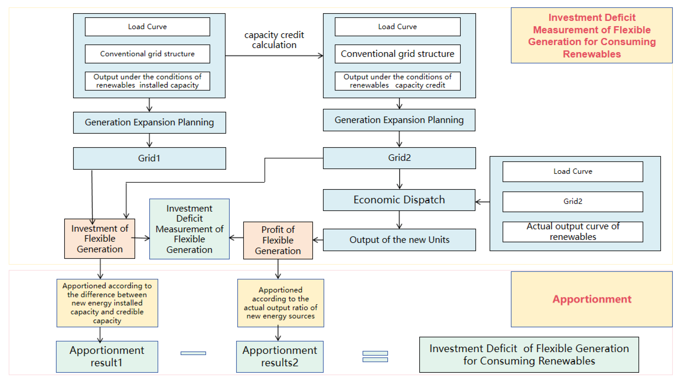
Based on the analysis of the investment cost gap of renewables’ flexible generation in 2.1, we obtained the investment cost gap calculation framework diagram of renewables’ flexible generation, as shown in Figure 1. By analyzing the output of renewables under the two extreme conditions of installed capacity and confidence capacity, we conducted power planning for renewables to obtain grid structures 1 and 2, respectively. By comparing the two grid structures, the investment of the supporting power supplies is obtained. Under the conditions of grid structure 2, using the actual curve of the renewables as the input, the output of the new units and the power generation benefits of the flexible generation are obtained through economic dispatch. Finally, the consumption cost of the renewable supporting power is obtained by calculating the difference between the investment of supporting power and the flexible generation.

2.2. Assessment Method of the Investment Gap for Flexible Generation for Renewables

2.2.1. Effective Load Carrying Capability

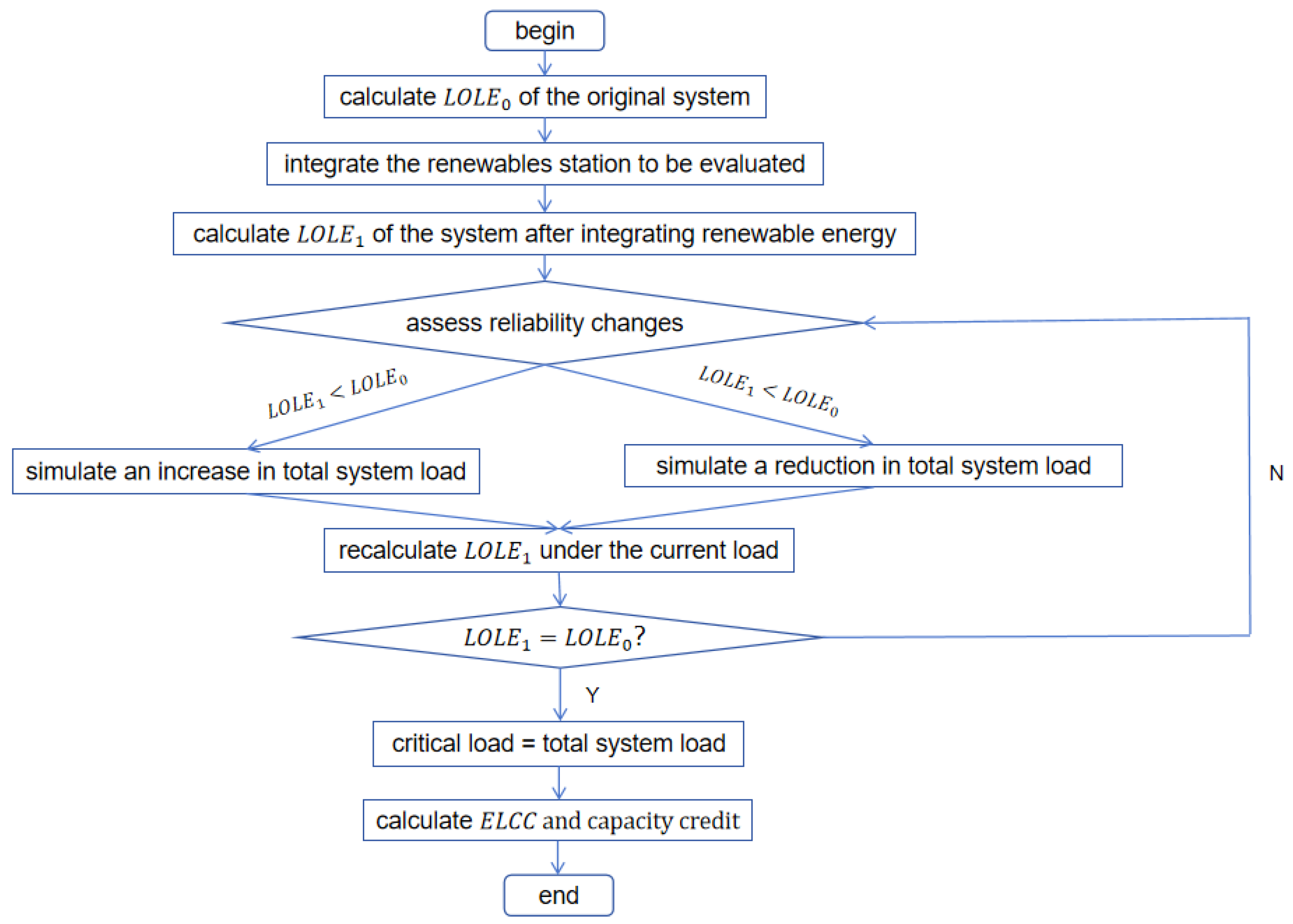
To scientifically assess the actual contribution of renewable energy to the long-term power supply adequacy of the electric power system, this study employs the effective load carrying capability (ELCC) method to calculate its credible capacity. This method is a rigorous evaluation framework based on system reliability criteria. Its core concept lies in quantitatively analyzing how much additional load can be equivalently supported by newly added renewable energy capacity under the premise of maintaining the same level of power system reliability. This incremental load is regarded as the “effective load carrying capability” of the renewable energy, representing its net contribution to system capacity adequacy, i.e., the credible capacity. The calculation process of this study is illustrated in Figure 2.

$$ELCC=L_{new}-L_{base}$$

(1)

$$\mathrm{capacity} \mathrm{credit}={\displaystyle \frac{ELCC}{\mathrm{rated} \mathrm{installed} \mathrm{capacity} \mathrm{of} \mathrm{the} \mathrm{renewables} \mathrm{Station}}}\times 100\%$$

(2)

$ELCC$ is the effective load carrying capability; $L_{new}$ refers to the maximum load the system can withstand while maintaining the same $LOLE$ as the baseline system; and $L_{base}$ is the total load of the original system.

2.2.2. Generation Expansion Planning Model

The two-stage power planning model considers the investment and operation stages, respectively. The objective function minimizes the expected value of the total system cost, which is the sum of the annual investment cost and the horizontal annual operating cost. Among them, the annual investment cost depends on the annual investment cost of thermal power units. The horizontal annual operating cost depends on the annual operation, maintenance cost, and fuel cost of thermal power units, the annual operation and maintenance cost of transmission lines, the annual load loss penalty, the annual wind and light abandonment cost, and the start-up and stop costs of thermal power units. Equation (12) considers the investment cost return rate and allocates the total system cost of each year according to the equipment life and discount rate. Planning models seek resource allocation options that minimize system costs. In this article, the output of renewables based on the installed capacity is taken as Condition 1, and the output of renewables based on reliable capacity is taken as Condition 2. As shown in Figure 3, in the method discussed in this paper, the load curves in the two cases are the input of the generation expansion planning model, and the output is the installed capacity of the flexible generation in the two cases.

• Objective Function:

$$\min C=C^{IN}+C^O$$

(3)

$$C^{IN}={\displaystyle \sum _{\mathrm{g}\in {\psi }_T}{c}_{R{F}_T}{c}_g^{in}{A}_g^{opt}{Y}_g}$$

(4)

$$\begin{array}{l}{C}^O={\displaystyle \sum _{g\in {\psi }_T}{c}_g^{om}{A}_g{Y}_g}+{\displaystyle \sum _{l\in \Gamma }{c}_l^{om}{L}_l}+\\ {\displaystyle \sum _{d\in D}{\omega }_d}{\displaystyle \sum _{t\in \Gamma }{\displaystyle \sum _{g\in {\psi }_T}{b}_g{P}_{g,d,t}}}+{\displaystyle \sum _{d\in D}{\omega }_d}{\displaystyle \sum _{t\in T}{\displaystyle \sum _{n\in N}{c}_n^{cur}{\zeta }_{n,d,t}}}+\\ {\displaystyle \sum _{d\in D}{\omega }_d}{\displaystyle \sum _{t\in T}{\displaystyle \sum _{g\in \psi }\left(c_g^{on}O{N}_{g,d,t}+c_g^{off}OF{F}_{g,d,t}\right)}}\end{array}$$

(5)

$$c_{RF}={\displaystyle \frac{r{\left(1+r\right)}^F}{{\left(1+r\right)}^F-1}}$$

(6)

$\mathrm{g}$, $\mathrm{n}$, $l$, $t$, and $d$ are units, regions, transmission lines, time periods, and scenarios; ${\psi }_T$, $N$, $\Gamma$, $T$, and $D$ are the thermal power unit collection, regional collection, transmission line collection, time period collection, and scene collection, respectively; $C$ is the total system cost; $C^{IN}$ is the total system investment cost; $C^O$ is the total system operating cost; $c_{R{F}_T}$ and $c_{R{F}_l}$ are the capital recovery coefficients of traditional units and transmission lines; $c_g^{in}$ is the investment per unit capacity of the unit; $c_g^{om}$ is the cost of ensuring the supply and demand for the area unit capacity; $A_{\mathrm{g}}^{opt}$ is the assembled capacity for the machine to be built; $A_{\mathrm{g}}$ is the installed capacity for all units; $c_l^{in}$ is the unit investment cost for transmission lines; $L_l$ is the transmission capacity of transmission lines; $c_l^{om}$ is the transmission line operation and maintenance cost per unit capacity; $c_n^{cur}$ is the cost of ensuring the supply and demand for the area $n$ unit capacity; ${\zeta }_{n,d,t}$ is the guaranteed supply demand power of area $n$ in scenario $d$ during period $t$; $b_g$ is the power generation cost coefficient of the unit; the power generation cost of the unit is approximated by a linear function; $P_{g,d,t}$ is the output of unit $\mathrm{g}$ in scenario $d$ during period $t$; ${\omega }_d$ is the number of days for the scene $d$ to last; $c_g^{on}$ and $c_g^{off}$ are the start-up cost and shutdown cost of the unit $\mathrm{g}$, respectively; and $O{N}_{g,d,t}$ is a binary variable indicating whether the unit $\mathrm{g}$ changes from the shutdown state to the on state during the period $t$ of the scene $d$, and its value is one, which means that the unit changes from the shutdown state to the on state during the scene period. Otherwise, this action will not occur. $OF{F}_{g,d,t}$ is whether unit $\mathrm{g}$ of unit $t$ changes from the on–on state to the off state during period $d$ of the levy scenario; otherwise this action will not occur. $Y_{\mathrm{g}}$ is a binary variable indicating whether the unit $\mathrm{g}$ is invested in construction; a value of one indicates the decision to invest in the construction of the unit. Otherwise, it will not be invested in construction.

2.

Constraint:

The power planning model builds a multi-dimensional investment and operation constraint system, including power balance constraints, unit output upper and lower limit constraints, load loss constraints, unit start–stop constraints, thermal power unit climbing constraints, transmission line safety constraints, and energy storage technology constraints, which are expressed as follows:

$${\displaystyle \sum _{\mathrm{g}\in {\psi }_n}{P}_{g,d,t}}+{\displaystyle \sum _{l\in {\Gamma }_{\mathsf{\partial }}}{F}_{l,d,t}}+{\displaystyle \sum _{n\in {\Gamma }_{in}}{P}_{n,d,t}^{outsi}}=L_{n,d,t}-{\zeta }_{n,d,t},\forall n,d,t$$

(7)

The formula is the power balance constraint. ${\psi }_n$ is the set of all units in the area $n$, $L_{n,d,t}$ is the load of area $n$ in scene $d$ during period $t$, ${\Gamma }_n$ is a subset of transmission lines with area $n$ as the first or last area, $P_{n,d,t}^{outsi}$ is the electric power provided outside the area $n$ in the scene $d$ and period $t$, and $P_{n,d,t}^{out,\max }$ and $P_{n,d,t}^{in,\max }$ are the maximum outflow value and the maximum inflow value of electric power in area $n$ during period $t$ of scene $d$.

$${\gamma }_{\mathrm{g}}^{\min }{A}_g{Y}_{g}S{T}_{g,d,t}\le P_{g,d,t}\le A_g{Y}_{g}S{T}_{g,d,t}$$

(8)

The formula is the unit upper and lower limit constraints. ${\gamma }_{\mathrm{g}}^{\min }$ represents the minimum output level of the unit.

There is a product of $Y_{\mathrm{g}}S{T}_{g,d,t}$ two binary variables in the constraint, which leads to a significant reduction in model calculation efficiency, so it is necessary to linearize $Y_{\mathrm{g}}S{T}_{g,d,t}$. The conventional linearization method used in this project is expressed as follows:

$$\begin{array}{l}\mathrm{y}=x_1{x}_2,x_1\in \left\{0,1\right\},x_2\in \left\{l,u\right\},l\ge 0\\ \left\{\begin{array}{l}y\le x_2\\ y\ge x_2-u\left(1-x_1\right)\\ l{x}_1\le y\le u{x}_1\end{array}\right.\end{array}$$

(9)

Applied to the upper and lower limits of unit output in this model, it is expressed as follows:

$$\begin{array}{l}{Y}_{\mathrm{g}}S{T}_{g,d,t}=Y_{g}S{T}_{g,d,t},Y_g\in \left\{0,1\right\},S{T}_{g,d,t}\in \left\{0,1\right\}\\ \left\{\begin{array}{l}{Y}_{g}S{T}_{g,d,t}\le Y_g\\ Y_{g}S{T}_{g,d,t}\le S{T}_{g,d,t}\\ Y_{g}S{T}_{g,d,t}\in \left\{0,1\right\}\end{array}\right.\end{array}$$

(10)

$$0\le {\zeta }_{n,d,t}\le L_{n,d,t},\forall n,d,t$$

(11)

Equation (17) is the load loss constraint.

$$\left\{\begin{array}{l}-OF{F}_{\mathrm{g},d,t}\le S{T}_{g,d,t}-S{T}_{g,d,t}\le O{N}_{g,d,t}\\ O{N}_{g,d,t}+OF{F}_{g,d,t}\le 1\end{array}\right.$$

(12)

$$S{T}_{\mathrm{g},d,t}\ge {\displaystyle {\sum }_{v=t-o{n}_g^{\min }}^{t}O{N}_{g,d,v}},\forall g\in {\psi }_T,d,t$$

(13)

$$1-S{T}_{\mathrm{g},d,t}\ge {\displaystyle {\sum }_{v=t-of{f}_g^{\min }+1}^{t}OF{F}_{g,d,v}},\forall g\in {\psi }_T,d,t$$

(14)

$${\displaystyle {\sum }_{t=T_{begin}}^{T_{end}}\left(O{N}_{g,d,t}+OF{F}_{g,d,t}\right)}\le CH{G}_g^{\max },\forall g\in {\psi }_T,d,t$$

(15)

$$S{T}_{\mathrm{g},d,t}O{N}_{g,d,t}OF{F}_{g,d,t}\in \left\{0,Y_g\right\},\forall g\in {\psi }_T,d,t$$

(16)

Equations (18)–(22) are the unit start and stop constraints. $S{T}_{\mathrm{g},d,t}$ is a binary variable that represents whether the unit $\mathrm{g}$ is on during the scenario $d$ period $t$. Its value is one, which means that the unit $\mathrm{g}$ is running; otherwise, it is in a shutdown state. $o{n}_g^{\min }$ and $of{f}_g^{\min }$ are the minimum continuous power-on time and the minimum continuous downtime respectively, $\left[T_{begin},T_{end}\right]$ is the beginning and end of the scene, and $CH{G}_{\mathrm{g}}^{\max }$ is the maximum number of starts and stops of the unit in a day.

$$-DW{P}_{\mathrm{g}}\le P_{\mathrm{g},\mathrm{t}}-P_{g,t-1}\le UP{P}_g,\forall g\in {\psi }_T,d,t$$

(17)

Equation (23) is the unit climbing constraint. $UP{P}_{\mathrm{g}}$ and $DW{P}_{\mathrm{g}}$ are the maximum allowable increase and decrease in the output power of the traditional unit.

$$\left|F_{l,d,t}\right|\le L_l,\forall l,d,t$$

(18)

Equation (24) is transmission line safety constraint. $F_{l,d,t}$ is the line power flow value of transmission line $l$ during period $t$ in scenario $d$.

2.2.3. Economic Dispatch Model

The economic dispatching model is established on the basis of the generation expansion planning model, taking the installed capacity of the flexible generation and the real load curve as the input, with the output being the output of each unit, as shown in Figure 4.

• Objective Function:

$$\begin{array}{ll}\hfill C& ={\displaystyle {\sum }_{\mathrm{t}=1}^T{\displaystyle {\sum }_{g=1}^G{C}_g\left(p_{g,t}\right)+}}{\displaystyle {\sum }_{t=1}^T{S}_{bp}{\epsilon }_{bp}}+{\displaystyle {\sum }_{t=1}^T{\displaystyle {\sum }_{f=1}^L{S}_{l,p}\left({\epsilon }_{lp}^{+}+{\epsilon }_{lp}^{-}\right)}}\\ & +{\displaystyle {\sum }_{t=1}^T{S}_{rp}{\epsilon }_{rp}}\\ & ={\displaystyle {\sum }_{t=1}^T{\displaystyle {\sum }_{g=1}^G{a}_g+b_{g,t}+c_g{p}_{g,t}^2+}}{\displaystyle {\sum }_{t=1}^T{S}_{bp}{\epsilon }_{bp}}\\ & +{\displaystyle {\sum }_{t=1}^T{\displaystyle {\sum }_{f=1}^L{S}_{lp,l}\left({\epsilon }_{lp}^{+}+{\epsilon }_{lp}^{-}\right)}}+{\displaystyle {\sum }_{t=1}^T{S}_{rp}{\epsilon }_{rp}}\end{array}$$

(19)

$a_g$, $b_g$, and $c_g$ are constant coefficients; $N$ is the total number of generators in the system; $p_{g,t}$ is the active power of the generator $g$ at the moment $t$; $S_{bp}$, $S_{lp,l}$, and $S_{rp}$ are constants that take maximum values; ${\epsilon }_{bp}$ is the power balance slack variable; ${\epsilon }_{lp}^{+}$ is the line power positive slack variable;${\epsilon }_{fp}^{-}$ is the line power negative slack variable; and ${\epsilon }_r$ is the capacity reserve slack variable.

2.

Constraint:

$${\displaystyle {\sum }_{g=1}^G{p}_{g,t}+{\epsilon }_{bp}={\displaystyle {\sum }_{i=1}^N{P}_{i,t}^d}},{\epsilon }_{bp}\ge 0$$

(20)

$$P_{f,t}=T_{f-1}\cdot \left({\displaystyle {\sum }_{g=1}^G{p}_g}-P_i^d\right)$$

(21)

$$T_{f-1}=M\cdot X\cdot C^T$$

(22)

$$-P_f^{\max }-{\epsilon }_{fp}^{+}\le P_{f,t}\le P_f^{\max }+{\epsilon }_{fp}^{-},{\epsilon }_{fp}^{+}\ge 0,{\epsilon }_{fp}^{-}\ge 0$$

(23)

$${\displaystyle {\sum }_{g=1}^G{r}_{g,t}+{\epsilon }_{rp}}\ge R_t,{\epsilon }_{rp}\ge 0$$

(24)

$$p_{g,t}-p_{g,t-1}\le R_{u,g}D$$

(25)

$$p_{g,t-1}-p_{g,t}\le R_{d,g}D$$

(26)

Equations (2)–(4) represent the power balance constraints. Equation (5) represents the line transmission constraints. Equation (6) represents the reserve constraints. Equations (7) and (8) represent the power balance constraints. $N$ is the number of nodes, $P_{f,t}$ is the power transmitted by the line $f$ during the period $t$, $P_t^{\max }$ the maximum power transmitted by the line $f$ during the period $t$, $P_{i,t}^d$ is the power transmitted by the node $i$ during the period $t$, $a_f$ is the power transmission distribution coefficient, $r_{g,t}$ is the spinning reserve capacity provided by the generator $g$ during the period $t$, $R_t$ is the spare capacity required by the system $t$, $R_{u,g}$ is the ramp rate of the generator $g$, $R_{d,g}$ is the landslide rate of the generator $\mathrm{g}$, and $D$ is the ramp time interval.

2.2.4. Investment Deficit Measurement Model

Incorporating environmental benefits and auxiliary service fees into the profit calculation of the power system reflects the economic inevitability of the evolution of power commodities from a single homogeneous energy product to a multi-dimensional heterogeneous service combination. The traditional dispatching model only focuses on minimizing fuel costs. Essentially, it regards electricity as an undifferentiated commodity, ignoring the environmental externalities and system service value that are inevitably associated with its production and consumption process. From an economic perspective, the monetization of environmental benefits is an essential means to correct market failure. If negative externalities such as carbon emissions and pollutant emissions are not internalized as enterprise costs, it will lead to society bearing hidden environmental debts and will distort the efficiency of resource allocation. The separate pricing of ancillary services reflects the product stratification logic of the modern power market. System services such as frequency regulation, reserve, and voltage support are actually derivatives that ensure power quality and system reliability. Their value needs to be discovered through independent price signals to avoid cross-subsidies among services of different attributes. This not only concerns the improvement of the corporate profit structure, but also affects whether the electricity market can form a full-cost price signal to guide long-term investment towards low-carbon and flexible resource types, thereby achieving the harmonious unity of the energy “impossible triangle”—economy, security, and sustainability—in a dynamic balance.

$$C^I=C_2^I-C_1^I$$

(27)

$$\begin{array}{l}\left\{\begin{array}{l}{P}_{\mathrm{a}ctual}=P_{\mathrm{theoretical}}\times \left(1-\gamma \right)\\ C_{output}=P_{actual}\times c_{output}\\ C_{green}=P_{actual}\times c_{green}\\ \mathrm{Cos}{t}_{aux}=P_{actual}\times c_{aux}\\ \mathrm{Cos}{t}_{ope}=P_{actual}\times c_{ope}\\ \mathrm{Pr}ofit=C_{output}+C_{green}-\mathrm{Cos}{t}_{aux}-\mathrm{Cos}{t}_{ope}\\ C^O=\mathrm{Pr}ofi{t}_2-\mathrm{Pr}ofi{t}_1\end{array}\right.\end{array}$$

(28)

$$C=C^I-C^O$$

(29)

$C_1^I$ and $C_2^I$ are the power planning investments when renewables sources are produced based on the installed capacity and based on the credible capacity, $P_{theoretical}$ is theoretical electricity settlement volume of new units, and $P_{actual}$ is actual electricity settlement volume. $\gamma$ is power curtailment rate, $C_{output}$ is the electrical energy income, $C_{green}$ is the environmental benefits, $c_{output}$ is the market price, $c_{green}$ is the green premium, $\mathrm{Cos}{t}_{aux}$ is the total auxiliary service fee, $\mathrm{Cos}{t}_{ope}$ is the operating cost, $c_{aux}$ is the auxiliary service fee, and $c_{ope}$ is the operating cost. $\mathrm{Pr}\mathrm{o}fit$ is the income of the new units, $\mathrm{Pr}\mathrm{o}fi{t}_1$ is the income of the new units in grid 1, $\mathrm{Pr}\mathrm{o}fi{t}_2$ is the income of the new units in grid 2, $C^O$ is the difference in the power generation income from the newly added units, and $C$ is the investment deficit of flexible generation for consuming renewables.

3. Results

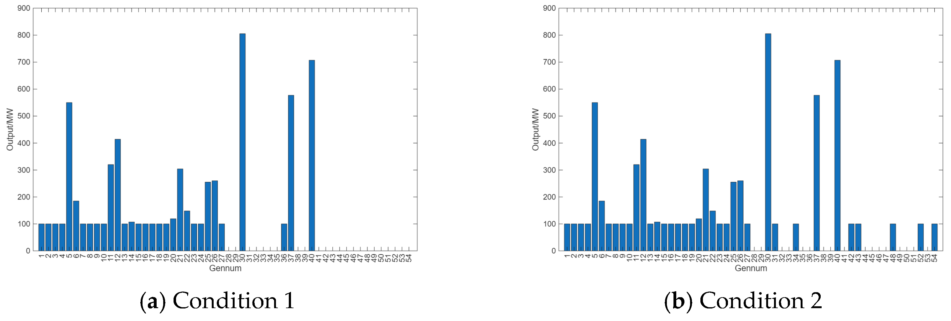
We used IEEE118 to conduct simulation analysis of this model. This study adopts the following key assumptions. Referring to the relevant literature, the construction cost of a single-cycle gas turbine is 404.6 million yuan, that of a combined cycle gas turbine is 797.06 million yuan, and that of a thermal power plant is 1416.10 million yuan. The fixed operating cost of a single-cycle gas turbine is 10.11 million yuan per year, that of a combined-cycle gas turbine is 19.92 million yuan per year, and that of a thermal power plant is 35.4 million yuan per year. In terms of technical parameters, the minimum output of single-cycle units is 39 MW, that of combined-cycle units is 46 MW, and that of thermal power is 105 MW. The ramping rate of single-cycle units is 1.5%, that of combined-cycle units is 7.4%, and that of thermal power units is 2.2%. The discount rate is 8%. Among them, the installed capacity of renewables and the installed capacity of traditional power units simulate the ratio of renewables and the traditional thermal power installed capacity in Henan Province. Through simulation, power planning decisions are obtained in two situations: when renewables sources are output according to unit capacity, and when output is based on credible capacity, as shown in

Table 1. Generation expansion planning.

Gen-num	28	29	30	31	32	33	34	35	36
Capacity	491	492	805.2	100	100	100	100	100	100
Plan1	0	0	1	0	0	0	0	0	0
Plan2	0	0	1	1	0	0	1	0	0
Gen-num	37	38	39	40	41	42	43	44	45
Capacity	577	100	104	707	100	100	100	100	352
Plan1	1	1	0	1	0	0	0	0	0
Plan2	1	0	0	1	0	1	1	0	0
Gen-num	46	47	48	49	50	51	52	53	54
Capacity	140	100	100	100	100	136	100	100	100
Plan1	0	0	1	0	0	0	1	0	1
Plan2	0	0	1	1	0	0	1	0	0

. Among them, decision 1 is the planning decision result of the unit to be planned when the renewable source is output according to the unit capacity, and decision 2 is the planning decision result of the unit to be planned when the renewable source is output according to the credible capacity.

As shown in Table 1, decision 1 added four new units, namely No. 30, No. 37, No. 38, and No. 40, to the existing units. Decision 2 added ten new units, namely No. 30, No. 31, No. 34, No. 37, No. 40, No. 42, No. 43, No. 48, No. 52, and No. 54. The planned capacities of each unit in the two scenarios are presented more intuitively in Figure 1. The planned capacity of each unit in the two situations is shown in Figure 5.

The installed capacity to be planned is 1612.2 MW when renewable sources are based on unit capacity, and the installed capacity to be planned when renewable sources are based on credible capacity is 3389.2 MW, as shown in Figure 6. Through calculation, the planned investment cost when renewables are output according to unit capacity is 303.47 million yuan, and the planned investment cost when renewables are output according to credible capacity is 304.64 million yuan, a difference of 1.17 million yuan.

Through power planning, new grid structures are obtained in the two situations. The grid structure when renewable sources are output according to installed capacity is called grid structure 1, and the grid structure when renewables sources are output according to trusted capacity is called grid structure 2.

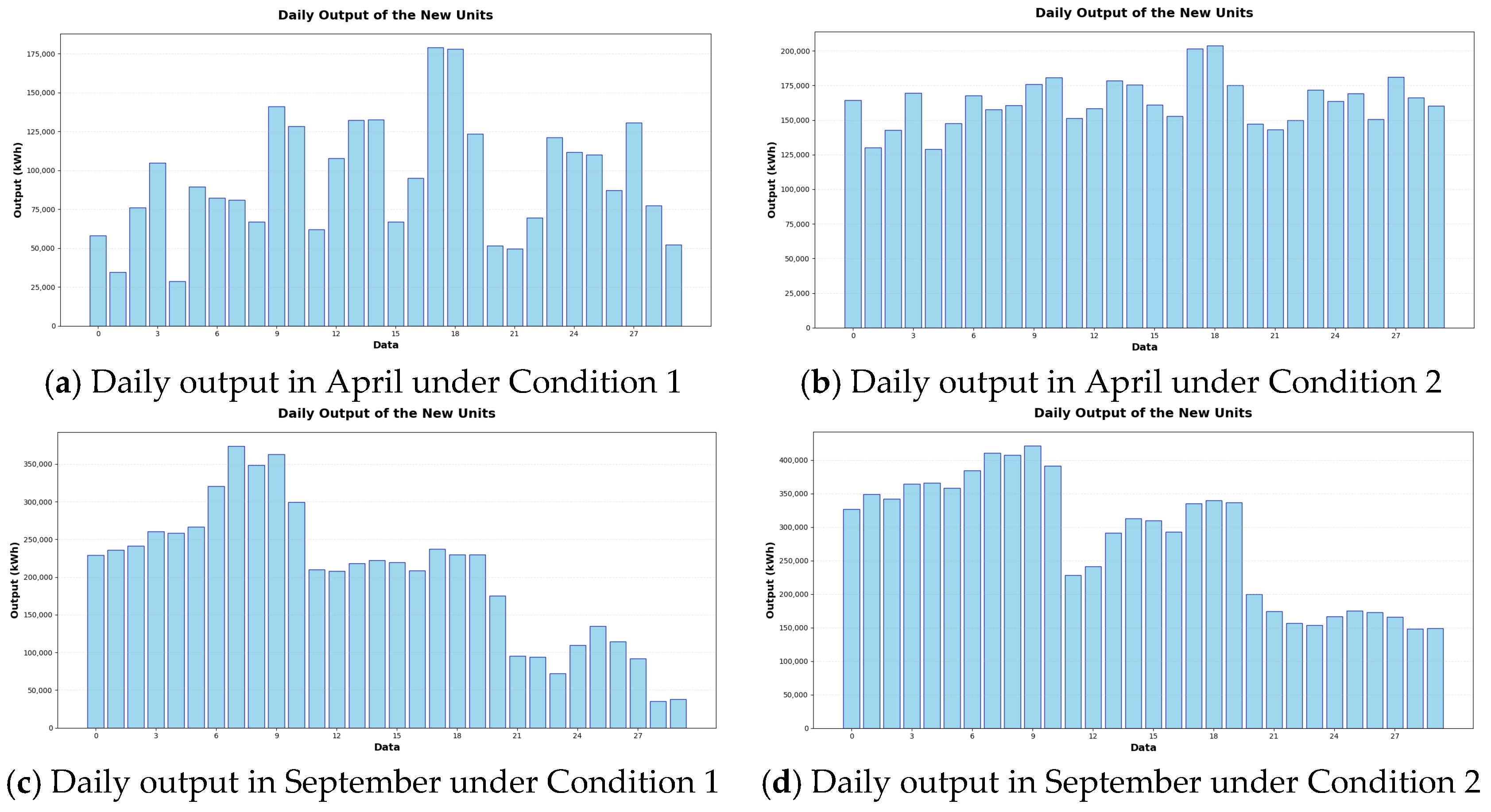
Through simulation, the output of the newly added units in each month under the two grid structures can be obtained, as shown in Figure 5.

From Figure 7, it can be observed that in the same month, the output trends of the units in the two situations are roughly the same, with the output under grid structure 2 being greater than that under grid structure 1.

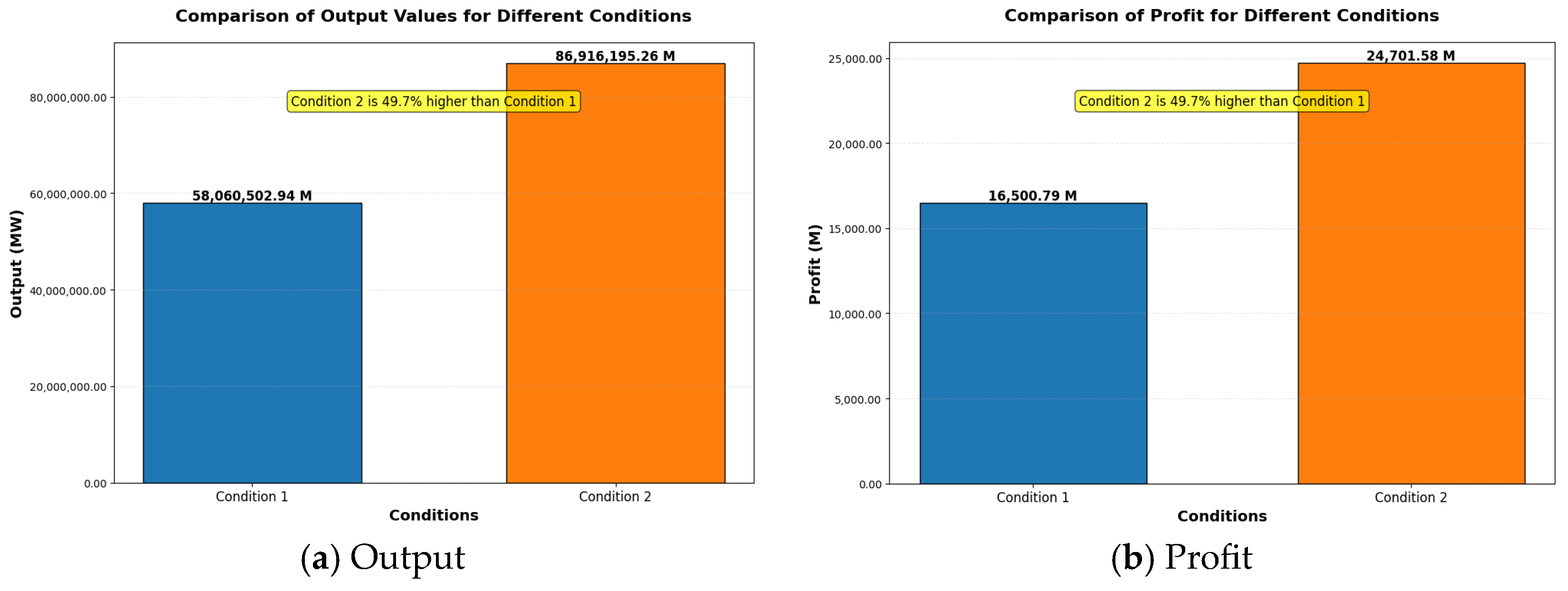
By summarizing the output of the newly added units in each month, the annual power generation and revenue of the newly added units can be obtained, as shown in Figure 8 Among them, the power generation of the newly added units under grid structure 1 is 58,060,503 MWH, and the revenue is 16,501 million. Under grid structure 2, the power generation of the newly added units is 869,16,195 MWH, and the revenue is 24,702 million. The difference in returns between the two cases is 8201 million. Combining the investment difference, the investment difference for renewables supporting power sources is 108,799 million.

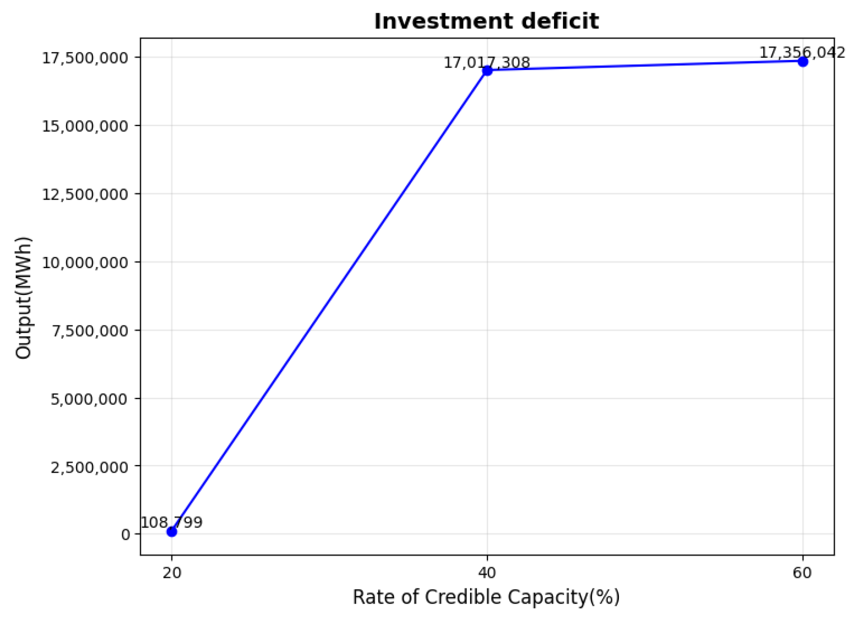
The results of the model’s sensitivity analysis are shown in Figure 9 and the model demonstrates a high degree of feasibility.

4. Discussion

The installed capacity of renewables is 1575 MW, while the planned installed capacity of renewables based on the unit capacity output is 1612.2 MW and the planned installed capacity based on the reliable capacity output is 3389.2 MW. It can be seen from this that the flexible generation of renewables is of great significance to the safe operation of the system.

Through this method, the cost difference in the flexible generation for renewables has been calculated, providing a new idea for the calculation of the cost of renewables’ consumption. For other power sources, such as energy storage, this method can also be referred to. In this article, a method for calculating the cost of consuming the supporting energy storage power supply is presented. Due to the randomness and volatility of the output of renewables, during its grid connection process, other power sources need to be matched with it to achieve real-time load balance. Energy storage has the characteristic of being capable of charging and discharging. If it is used as a supporting power source, by analogy with the idea of using thermal power as a supporting power source in this study, investment in and the transformation of the power grid are required, which will generate investment and construction costs. However, the newly built energy storage can bring certain profits during the power generation process, and this part of the profits can recover part of the investment and construction costs. Therefore, the difference between the investment and construction cost of the supporting energy storage power supply and the power generation revenue is regarded as the consumption cost of the renewables supporting energy storage power supply.

Since the construction and transformation of renewables is positively correlated with the installed capacity and reliable capacity of renewables stations, and the greater the difference between the two, the higher the investment and construction cost of renewables; the investment and construction cost of the flexible generation is allocated according to the size of the difference between the installed capacity and reliable capacity of the renewables station. As shown in Figure 10, the output of thermal power units is negatively correlated with the actual output of renewable stations. The more the output of renewable stations, the less the output of thermal power units. Therefore, the revenue of thermal power units should be allocated in reverse according to the output of renewable stations. The difference between the allocated investment and construction costs of the supporting power sources for each renewable station and the power generation revenue is the difference in the allocated investment and construction costs of the supporting power sources.

5. Conclusions

This study proposes a method for calculating the investment deficit of supporting power sources for renewables. To ensure the reliability of the concealed nature of the power grid, we conduct the calculation under two scenarios: the output of renewables based on the installed capacity and the output based on the reliable capacity. The new grid structure and investment cost of the newly added units are obtained through the power supply planning model, and the output situation and revenue of the newly added units are obtained through the economic dispatching model. The final investment difference in the flexible generation for renewables is obtained. In the simulation analysis, by simulating the installed capacity ratio of renewables to thermal power units in Henan Province, the data is made to be more in line with the actual situation of Henan Province. Through calculation, the investment deficit of the renewable units in the two cases, the income difference, and the investment deficit of the flexible generation are obtained. This study provides ideas to calculate construction and renovation costs in the cost estimation of renewables’ consumption. Additionally, it calculates the investment deficit of flexible generation for consuming renewables. The feasibility of this method was verified through sensitivity analysis. Based on this method, we proposed the idea of cost sharing for the subsequent consumption of renewables, laying a foundation for the subsequent cost sharing work of consumption. At the same time, we suggested that the cost calculation of other types of supporting power sources could be compared with the method in this study. This study has facilitated a comprehensive calculation of the cost of renewables’ consumption, while the subsequent research on the allocation work needs to be further elaborated in detail.

References

1. Chen, S.Q.; Kharrazi, A.; Liang, S.; Fath, B.D.; Lenzen, M.; Yan, J.Y. Advanced approaches and applications of energy footprints toward the promotion of global sustainability. Appl. Energy 2020, 261, 114415. [Google Scholar] [CrossRef]
2. Tseng, M.L.; Tran, T.P.T.; Ha, H.M.; Bui, T.D.; Lim, M.K. Sustainable industrial and operation engineering trends and challenges Toward Industry 4.0: A data driven analysis. J. Ind. Prod. Eng. 2021, 38, 581–598. [Google Scholar] [CrossRef]
3. Zhou, J.G.; Li, L.; Tseng, M.L.; Ahmed, A.; Shang, Z.X. A novel green design method using electrical products reliability assessment to improve resource utilization. J. Ind. Prod. Eng. 2021, 38, 561–572. [Google Scholar] [CrossRef]
4. Jiang, X.L.; Li, Y.C.; He, Y.Z. Evaluation of power system equivalent inertia considering renewables virtual inertia. J. Electr. Power Sci. Technol. 2023, 38, 169–176. [Google Scholar]
5. Lin, F.; Xiao, L.H.; Shang, H.L.; Xu, C.; Luo, Z.D.; Chen, J.J.; Ma, X.F. Design and application of energy internet digital twin system under the background of dual carbon. J. Electr. Power Sci. Technol. 2022, 37, 29–34. [Google Scholar]
6. EirGrid Plc. System and Renewable Data Summary Report [Data File]. 2021. Available online: https://www.eirgridgroup.com/site-files/library/EirGrid/System-and-Renewable-Data-Summary-Report.xlsx (accessed on 15 March 2022).
7. EirGrid Plc.; SONI Ltd. All-Island Generation Capacity Statement [Online Report]. 2021. Available online: https://cms.eirgrid.ie/sites/default/files/publications/208281-All-Island-Generation-Capacity-Statement-LR13A.pdf (accessed on 12 July 2022).
8. Cao, J.; Gao, J.M. Coordination mechanism and simulation of household photovoltaic county development based on evolutionary game. Power Syst. Technol. 2023, 47, 669–684. [Google Scholar]
9. Chen, C.; Fu, X.W.; Zhou, W.H. Two-staged generation-grid-load-energy storage interactive optimization operation strategy for promotion of distributed photovoltaic consumption. Power Syst. Technol. 2022, 46, 3786–3799. [Google Scholar]
10. Feng, Z.S.; Zhang, Z.H.; Guo, Y.H. Status and prospect of China’s wind power development in 2021. Water Power 2022, 48, 1–3+8. [Google Scholar]
11. Li, J.; Ho, M.S. Indirect cost of renewable energy: Insights from dispatching. Energy Econ. 2022, 105, 105778. [Google Scholar] [CrossRef]
12. Liu, Y.; Xia, B.; Xu, L.; Zheng, Z. Analysis of renewable energy’s development in China and quantitative prediction of the power balancing gap. In Proceedings of the 2024 6th International Conference on Power and Energy Technology (ICPET), Beijing, China, 12–15 July 2024; pp. 1107–1111. [Google Scholar] [CrossRef]
13. Singh, N.K.; Koley, C.; Gope, S. Hybrid energy systems integrated power system imbalance cost calculation using moth swarm algorithm. In Smart Innovation, Systems and Technologies; Springer: Berlin/Heidelberg, Germany, 2023; Volume 316, pp. 49–59. [Google Scholar] [CrossRef]
14. Dai, X.; Zhang, K.; Geng, J.; Wang, Y.; Yuan, K. Calculating wind variability costs with considering ramping costs of conventional power plants. J. Electr. Eng. Technol. 2019, 14, 2267–2276. [Google Scholar] [CrossRef]
15. Gianfreda, A.; Parisio, L.; Pelagatti, M. A review of balancing costs in Italy before and after RES introduction. Renew. Sustain. Energy Rev. 2018, 91, 549–563. [Google Scholar] [CrossRef]
16. Ding, Y.; Shao, C.; Yan, J.; Song, Y.; Zhang, C.; Guo, C. Economical flexibility options for integrating fluctuating wind energy in power systems: The case of China. Appl. Energy 2018, 228, 426–436. [Google Scholar] [CrossRef]
17. Qu, J.; Shi, W.; Shan, W.; Zhang, Z.; Bai, H. Research on Renewables Operation Credible Capacity Evaluation and It’s Influence on Renewables Accommodation. In Proceedings of the 2023 5th Asia Energy and Electrical Engineering Symposium (AEEES), Chengdu, China, 23–26 March 2023; pp. 1582–1587. [Google Scholar] [CrossRef]
Figure 1. Assessment framework of the investment gap for flexible generation for renewables.
Processes 14 00516 g001
Figure 2. The calculation process of the credible capacity.
Processes 14 00516 g002
Figure 3. The input and output model of generation expansion planning.
Processes 14 00516 g003
Figure 4. The input and output model of economic dispatching.
Processes 14 00516 g004
Figure 5. The planned capacity of each unit in the two situations.
Processes 14 00516 g005
Figure 6. The installed capacity to be planned.
Processes 14 00516 g006
Figure 7. The output of the newly added units in each month.
Processes 14 00516 g007
Figure 8. The output and profit under two conditions.
Processes 14 00516 g008
Figure 9. Analysis of flexibility.
Processes 14 00516 g009
Figure 10. The appointment method of the investment deficit of flexible generation for consuming renewables.
Processes 14 00516 g010