Displacement Mechanism of Sequential Droplets on a Wetting Confinement

Abstract

The stability and uniformity of a liquid line formed by the sequential deposition of droplets are essential to the quality of products in many industry applications. In this work, a numerical model based on the front tracking method (FTM) is developed to investigate the displacement dynamics of sequential droplets on wetting confinement. We systematically examine the impact of wetting conditions and confinement width on the spreading length, morphology, and confined angle for a droplet. In addition, an analytical model is derived to predict the droplet displacement spacing for a uniform line. The analytical results align well with the numerical results, and the sequential droplets displaced with the predicted space achieve the minimum cross-section error and exhibit enhanced uniformity. Our numerical and analytical studies of droplet displacement within wetting confinement provide fundamental insights and a predictive framework for enhancing the uniformity and stability of liquid lines in precision manufacturing processes.

1. Introduction

A liquid line on a confined surface formed by the displacement of the sequential droplets is a fundamental problem in a number of industry applications, such as ink-jet printing [1,2], rapid prototyping [3,4], microfabrication [5,6], and electronic packaging [7,8]. All these applications require a continuous line with a uniform thickness since the morphology is essential to the production efficiency [9,10]. It is known that the forming process of a liquid line on a homogeneous surface shows instability. The capillary forces between touching droplets can relocate them from their original position [11], in which case the liquid line may break into individual droplets and develop bulges or even self-propelled jumping [12]. The uniformity of the liquid line depends mainly on the boundary conditions for the moving contact line and the droplet spacing [13].

Numerous research works have explored the displacement mechanism and the uniformity of the sequential droplets on a homogeneous surface by experimental observations and analytical modeling. Using linear hydrodynamic theory, Davis [14] first showed that a liquid line on a homogeneous surface is unstable when either a contact line with a constant angle moves freely or a contact line with a contact angle higher than $\pi /2$ is arrested in a parallel state. This boundary condition was verified by the experimental study of Schiaffino and Sonin [15], who displaced molten droplets onto a homogeneous solid surface with contact lines arrested parallelly, and found that the contact line is steady as the contact angle is smaller than $\pi /2$. Duineveld [16] studied another uniform type of a liquid line on a homogeneous substrate for a different bounding condition. In his work, the liquid had a zero receding contact angle, and his focus was on the formation of liquid bulges.

It is possible to obtain a uniform line by optimizing the droplet spacing [17,18,19]. Stringer and Derby [20] extended Duineveld’s model in the aspect of droplet spacing. They proposed that there are two limits of the spacing values: the maximum value for steady coalescence, and the minimum value for avoiding the forming of bulges. Soltman and Subramanian [21] presented an experimental investigation on the line shape on a homogeneous surface by varying the drop spacing, and found that the shape also varies from liquid bath, bulging, uniform, and discontinues lines to separate drops. Recently, Abunahla et al. [22] proposed a segmented and symmetric printing methodology for preventing liquid bulges during the formation of liquid lines. The liner displacement is divided into segments of three droplets. First, the two droplets at the ends are printed, and they are then connected by the third droplet in the center.

Over recent decades, substantial mathematical research has focused on multiphase flow and its practical applications. The literature presents a wide array of numerical methods for simulating two-phase flows. Among these are volume of fluid [23,24], diffuse interface [25], level set [26], phase field, and front-tracking techniques [27,28]. A key benefit of front-capturing methods is their inherent ability to manage topological changes in the interface without requiring special treatment [29]. Recently, Pan et al. [30] introduced a novel front-tracking approach termed the Edge-Based Interface Tracking (EBIT) method. Its lack of explicit connectivity makes it particularly suitable for near-automatic parallelization. However, accurately representing the contact angle has long been a challenge for the front-tracking method when dealing with gas–liquid–solid triple-phase interfaces. To address this issue, this work proposes a novel threshold-based approach for handling contact angle dynamics.

Thus far, both experimental and analytical studies have predominantly centered on homogeneous surfaces. It is known that the wetting condition of a fixed width with $\theta <\pi /2$ is essential for the uniformity of the liquid line [14]. However, it is not easy to achieve this condition on a homogeneous surface. Wang et al. [31] showed the effect of surface anisotropy on contact angles by depositing a droplet on grooved surfaces. In this work, we present an analytical model to predict droplet spacing for a uniform liquid line on hydrophilic confinement and perform numerical studies of the droplet displacement on the surface.

2. Numerical Model

2.1. Governing Equation

In this work, fluids are assumed to be incompressible, and the conservation equation of mass reads

$$\nabla ·\mathbf{u}=0,$$

(1)

where $\mathbf{u}$ denotes the fluid velocity. The momentum conservation equation for droplets and the ambient fluid is

$${\displaystyle \frac{\partial \rho \mathbf{u}}{\partial t}}+\nabla ·\left(\rho \mathbf{u}\mathbf{u}\right)=-\nabla p+\rho \mathbf{g}+\nabla ·\left[\mu (\nabla \mathbf{u}+\nabla {\mathbf{u}}^T)\right]+\mathbf{F},$$

(2)

where $\rho$ and $\mu$ indicate density and viscosity, respectively. $\mathbf{g}$ is the gravity acceleration, p is the pressure, and t is the time. The last term on the right-hand side is a singular body force $\mathbf{F}$, which is

$$\mathbf{F}=\sigma {\int }_s{\kappa }_f{\mathbf{n}}_f\delta (\mathbf{x}-{\mathbf{x}}_f)dS,$$

(3)

where $\sigma$ is the surface tension coefficient, ${\kappa }_f$ is the curvature, ${\mathbf{n}}_f$ is a unit vector normal to the front, and ${\mathbf{x}}_f$ denotes the position of the interface. The subscript s on the integral sign denotes integration over interfaces, and $\delta$ is a three-dimensional delta function identifying the interface location. Owing to the general misalignment between the interface and the Cartesian grid nodes, the surface tension force at each Lagrangian point is distributed over a cluster of surrounding cells (see Figure 1a) and subsequently imposed on the momentum equations of the adjacent nodes. Thus, the sharp delta function is effectively replaced by a smoothed distribution function, denoted D, for discrete meshes. The forcing at any grid point $\mathbf{x}(i,j,k)$ is then given by

$$\mathbf{F}(i,j,k)=\sigma \sum _{l=1}^m{\kappa }_f\left(l\right){\mathbf{n}}_f\left(l\right)D(\mathbf{x}(i,j,k)-{\mathbf{x}}_f\left(l\right)),$$

(4)

where l represents the lth number of the Lagrangian point on the interface, and m is the total Lagrangian point number. For our calculations, we use the distribution function

$$D(\mathbf{x}-\mathbf{x}\left(l\right))=\left\{\begin{array}{cc}{\left(4h\right)}^{(-\alpha )}\sum _{i=1}^{\alpha }\left(1+cos{\displaystyle \frac{\pi }{2h}}(x_i-x_i\left(l\right))\right),\hfill & \mathrm{if}|x_i-x_i\left(l\right)|<2h,i=1,\alpha ;\hfill \\ 0,\hfill & \mathrm{otherwise},\hfill \end{array}\right.$$

(5)

introduced by Peskin [32]. Here, h is the mesh width and $\alpha =3$ for three dimensions.

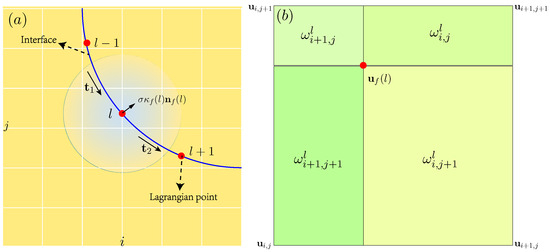
Figure 1. (a) Transfer of surface tension force from Lagrangian boundary point to surrounding fluid nodes; (b) velocity calculation of lth point from adjacent grid point by weighted value.

We use a marker function $I\left(\mathbf{x}\right)$ to differentiate between phases and their respective physical properties. Specifically, the function takes a value of 0 in the ambient fluid and 1 within the droplet. The mathematical formulation can be expressed as

$$\varphi \left(\mathbf{x}\right)={\varphi }_{drop}\left(\mathbf{x}\right)I\left(\mathbf{x}\right)+(1-I\left(\mathbf{x}\right)){\varphi }_{ambient}\left(\mathbf{x}\right),$$

(6)

where $\varphi$ represents $\rho$ and $\mu$. The jump of the physical properties at the interface is converted to a thin layer gradient, which can be written as

$$\nabla \varphi \left(\mathbf{x}\right)=({\varphi }_{drop}\left(\mathbf{x}\right)-{\varphi }_{ambient}\left(\mathbf{x}\right))\nabla I\left(\mathbf{x}\right)=\Delta \varphi \left(\mathbf{x}\right)\nabla I\left(\mathbf{x}\right),$$

(7)

where $\Delta \varphi \left(\mathbf{x}\right)={\varphi }_{drop}\left(\mathbf{x}\right)-{\varphi }_{ambient}\left(\mathbf{x}\right)$ indicates the jump of physical properties at the interface, and the $\nabla I\left(\mathbf{x}\right)$ is the gradient of the marker function, which can be expressed as

$$\nabla I\left(\mathbf{x}\right)=-\delta \left(n\right)\mathbf{n},$$

(8)

where n is the normal direction.

For each time step, as the interface position undergoes shifts and updates, the marker function will be reconfigured. Simultaneously, the associated fluid physical parameters on both sides of the interface will be adjusted accordingly.

2.2. Interface Tracking

The front tracking method employs two distinct grid systems: a Eulerian grid defined in Cartesian coordinates for resolving the governing equations, and a separate front grid that monitors the droplet interface. The process is initiated by defining the initial conditions, including fluid properties, the geometry of the interface, and other relevant parameters. During each computational cycle, the Navier–Stokes equations are solved on the Eulerian grid to update the velocity, density, viscosity, and indicator field. These computed values are subsequently interpolated onto the front grid (Equation (10)) to determine interface velocities and track its evolving position. Physical properties calculated on the front grid are then mapped back to the Eulerian grid via an interpolation scheme that accounts for the distance between the two grids. The resulting forces are incorporated into the Navier–Stokes equations, thereby influencing the subsequent fluid dynamics. This iterative cycle of updating both grids is repeated continuously until the final simulation time is attained [33,34].

FTM adopts a series of Lagrange marker points to explicitly track the interface. The marker points along the interface connect with each other in an orderly way, and the coordinate data ${\mathbf{x}}_f\left(l\right)$ reads

$${\mathbf{x}}_f\left(l\right)=(x\left(l\right),y\left(l\right),z\left(l\right)),l=1,2,\dots ,m.$$

(9)

Once we obtain the location of the marker points, the velocity ${\mathbf{u}}_f\left(l\right)$ can be calculated from the grid nodes by the bilinear interpolation

$${\mathbf{u}}_f\left(l\right)=\sum _{ijk}{w}_{ijk}{\mathbf{u}}_{ijk},$$

(10)

where $w_{ijk}$ and ${\mathbf{u}}_{ijk}$ are the weighted value and the velocity at the grid node $(i,j,k)$ of the exclusively used structured mesh, respectively. For the two-dimensional computations, the maker point divides the cell into four sub-cells as is shown in Figure 1b, and the weight value $w_{ij}$ is defined as the area of its diagonally opposite sub-cell. This method can be extended to three dimensions, where the weight would correspond to the volume of the diagonally opposite sub-volume. Then the maker points and interface can be moved and updated by

$${\mathbf{x}}_f^{t+\Delta t}\left(l\right)={\mathbf{x}}_f^t\left(l\right)+{\mathbf{u}}_f^t\left(l\right)\Delta t,$$

(11)

where $\Delta t$ is the time step.

2.3. Wetting Confinement

The wettability of a droplet on a flat surface is another issue that needs to be considered. Here, Young’s equation (Zhu et al. [35,36]) is introduced to describe the interfacial forces of the contact line, and it can be expressed by

$$\sigma cos\left({\theta }_Y\right)={\sigma }_{sv}-{\sigma }_{sl},$$

(12)

here, ${\theta }_Y$ is the equilibrium contact angle, which is determined by the chemical properties of the surface, and ${\sigma }_{sv}$ and ${\sigma }_{sl}$ are the surface tension of the solid/gas and solid/liquid interfaces, respectively. We introduce a threshold near the wall to apply interfacial stresses at marker points located in the vicinity of the threshold line (see Figure 2). The Lagrangian point l situated immediately above the threshold is highlighted in red. This point experiences a net surface tension force, denoted as $F_c\left(l\right)$, directed towards the center of the contact area. The horizontal and vertical components of the surface tension at the marker l are denoted as $F_{\tau }\left(l\right)$ and $F_z\left(l\right)$, respectively. According to the three-phase interface stress balance described by Equation (12), the corresponding stress components are given by

$$F_c\left(l\right)=\sigma cos\left({\theta }_Y\right),$$

(13)

$$F_{\tau }\left(l\right)=0,$$

(14)

$$F_z\left(l\right)=0.$$

(15)

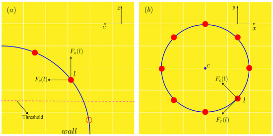
Figure 2. Force balance at the three-phase interface: (a) A threshold near the wall is introduced, and a net surface tension force of the the Lagrangian point l is denoted as $F_c\left(l\right)$ Within the c-z coordinate plane. (b) Components of the surface tension within the x–y plane from a top–down perspective.

No interfacial tension is applied to marker points situated below the threshold (marked by hollow cycle). The interfacial stresses computed from Equation (13) to (15) are then interpolated onto the grid nodes according to the positions of the marker points for subsequent iterative calculations.

2.4. Projection Method

The governing equation is solved through the project method, which is an efficient way to discretely solve the N-S equation of incompressible fluid. We introduce a intermediate velocity field ${\mathbf{u}}^{\ast }$, and the momentum conservation Equation (2) is decomposed by

$${\rho }^{n+1}{\mathbf{u}}^{\ast }-{\rho }^n{\mathbf{u}}^n=\Delta t(-{\mathbf{A}}_h^n+{\rho }^n\mathbf{g}+{\mathbf{D}}_h^n+{\mathbf{F}}_{\sigma }^n),$$

(16)

$${\rho }^{n+1}{\mathbf{u}}^{n+1}-{\rho }^{n+1}{\mathbf{u}}^{\ast }=-\Delta t{\nabla }_{h}p,$$

(17)

where the superscript n is the variable at time t. ${\mathbf{A}}_h^n$, ${\mathbf{D}}_h^n$ and ${\mathbf{F}}_{\sigma }^n$ are respectively the convection term, the diffusion term, and the body force. The grid spacing is h, and ${\nabla }_h$ is the approximation discretion of the gradient.

The ${\mathbf{u}}^{n+1}$ solved by Equation (17) should satisfy the incompressibility condition, namely

$${\nabla }_h{\mathbf{u}}^{n+1}=0.$$

(18)

Substituting Equations (18) into (17), we get

$${\nabla }_h\left({\displaystyle \frac{1}{{\rho }^{n+1}}}{\nabla }_{h}p\right)={\displaystyle \frac{1}{\Delta t}}{\nabla }_h{\mathbf{u}}^{\ast }.$$

(19)

The pressure field $p^{n+1}$ is calculated by Equation (19), and then substituting it to Equation (17), one can get the velocity field ${\mathbf{u}}^{n+1}$.

The Euler grid is applied to discretize the computational domain, and the finite volume method is used to apply the conservation of mass and momentum to the control unit with a small volume.

3. Results and Discussion

In this section, the numerical model based on FTM is verified by simulating a droplet spreading on a homogeneous surface, and comparing the dimensionless spread factors with the analytical results. Numerical computations of a droplet spreading on a wetting confinement are implemented to investigate the effect of confinement width and wetting angle on the spreading length. The evolution of the morphology is obtained. An analytical model is derived to predict the displacement spacing of a uniform liquid line on a hydrophilic confinement surface. The sequential droplets displaced with a predicted space is simulated, and the uniformity is analyzed. The characteristic length scale is $D_0$, which is the initial diameter of the droplet. The time scale is $D_0\mu /\sigma$. Then the dimensionless time $\dot{t}$ is defined as $\dot{t}=t\sigma /D_0\mu$. From here on, $\dot{}$ denotes dimensionless variables unless otherwise mentioned. The numerical simulations of a single droplet are performed in a computational domain of dimensions $5D_0\times 5D_0\times 5D_0$ resolved by a $100\times 100\times 100$ grid. Based on resolution studies reported in our previous work [37], we expect the results to be independent of the resolution.

3.1. Validation

To verify the numerical model, the spreading of a droplet on a homogeneous surface with different wetting angles $\theta$ is simulated here. In this work, the initial velocity is zero. The displaced droplet is assumed to be a spherical cap [18]. According to the volume conservation of the droplet [18], the dimensionless spread factor $\dot{D}$ of the spherical cap can be expressed as

$$\dot{D}={[{\displaystyle \frac{{(1-cos\left(\theta \right))}^2(2+cos\left(\theta \right))}{4{sin}^3\left(\theta \right)}}]}^{-1/3},$$

(20)

where $\dot{D}=D/D_0$, and D is the diameter of the equilibrium shape. Equation (20) shows that the spread factor $\dot{D}$ is just a function of the wetting angle $\theta$. We compare our numerical results with the theoretical values calculated from Equation (20) in Figure 3, which shows good agreement of the numerical results with the theoretical values.

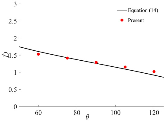
Figure 3. Comparison of the numerical results with the theoretical results. The solid line represents the theoretical results calculated by Equation (14), and the red points are the present numerical results.

3.2. Spreading on a Wetting Confinement

The liquid line is formed by the coalescence of a series of overlapping single droplets. Understanding the spreading of a single droplet on the confinement surface is essential to acquire the predicted droplet spacing for the uniform line. Here, we consider the confinement surface consisting of three regions with significant variation of wetting angle at the boundaries. As shown in Figure 2, the two side regions are set to be super-hydrophobic (blue color), while the middle region has the hydrophilic wetting angle $\theta$ (yellow color). Unlike the boundary condition of a droplet spreading on a homogeneous surface, the contact line perpendicular to the boundary of the confinement (y direction) is pinned, and the contact line parallel to the confinement (x direction) is free to move as shown in Figure 2. Here, we are only concerned about the condition where the confinement width W is smaller than the diameter D of a spherical cap droplet on a homogeneous surface. The spreading width is thus fixed by W. The maximum spreading length $L_{max}$, the confinement angle ${\theta }^{\ast }$, and the wetting angle $\theta$ of the confinement are all shown in Figure 4. $A^{\ast }\left(x\right)$ and $A\left(y\right)$ are the cross-sectional areas in the y and x directions, respectively.

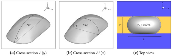
Figure 4. Spreading of a single droplet on a wetting confinement: (a) cross-section A(y) in x direction; (b) cross-section A^∗ $\left(x\right)$ in y direction; (c) top view of a droplet spreading on confinement. The blue and yellow colors represent super-hydrophobic and hydrophilic regions, respectively.

3.2.1. Prediction of the Spread Length

Here, an approximate geometric model based on volume conservation is derived to predict dimensionless spread in the x direction. The volume of the droplet $V_d$ can be expressed as the integral of the cross-section area $A\left(y\right)$ over the width W of the wetting confinement

$$V_d={\int }_{W}A\left(y\right)dy.$$

(21)

The cross-section area $A\left(y\right)$ in Equation (21) can be expressed straightforwardly in terms of the wetting angle $\theta$ and the local base length $L\left(y\right)$

$$A\left(y\right)=L^2\left(y\right){\displaystyle \frac{\theta -sin\left(\theta \right)cos\left(\theta \right)}{4sin\left(\theta \right)sin\left(\theta \right)}}.$$

(22)

See the work of GAO et al. [38] for a detailed derivation.

Substituting Equation (22) into (21) we can evaluate the integral. Here, however, we assume the spreading of the droplet on the wetting confinement is an approximate rectangle with length L and width W as shown in Figure 5. The approximate rectangle is marked by pink color, and the actual spread length is denoted as $L^{\ast }$. Under weak confinement, the droplet is expected to spread sufficiently, resulting in a spread length of $L^{\ast }=D_0$ (see Figure 5a). We can easily conclude that $L\approx 0.8D_0=0.8L^{\ast }$ based on the conservation of spreading area $S_s$

$$S_s=L{D}_0={\displaystyle \frac{\pi D_0^2}{4}},$$

(23)

under strong confinement, the two ends of the spread region are modeled as semicircles, with the central region remaining rectangular with $L\approx L^{\ast }$ (see Figure 5b). Therefore, we take an intermediate value $L=0.9L^{\ast }$, and simplify the integral by replacing $L\left(y\right)$ with an equivalent spreading length $L=0.9L^{\ast }$, which is constant. A volume correction factor $\epsilon$ is applied to the simplified integration

$${\int }_W{L}^2\left(y\right){\displaystyle \frac{\theta -sin\left(\theta \right)cos\left(\theta \right)}{4sin\left(\theta \right)sin\left(\theta \right)}}dy=\epsilon {L^{\ast }}^{2}W{\displaystyle \frac{\theta -sin\left(\theta \right)cos\left(\theta \right)}{4sin\left(\theta \right)sin\left(\theta \right)}},$$

(24)

where the value of $\epsilon =0.8$ can be obtained.

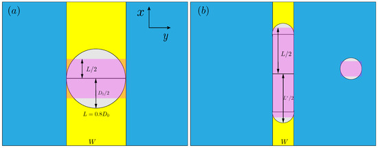
Figure 5. The spreading of a droplet under confinement, where yellow denotes hydrophobic regions and blue represents hydrophilic ones, is approximated as a rectangle of length L. The actual spread length, denoted $L^{\ast }$, is highlighted in pink: (a) Under weak confinement, the droplet is expected to spread sufficiently, resulting in a spread length of $L^{\ast }=D_0$. (b) Under strong confinement, the two ends of the spread region are modeled as semicircles, with the central region remaining rectangular.

Substituting Equation (24) into (21), the dimensionless spreading length $\dot{L}$ can be written as

$$\dot{L}=\sqrt{{\displaystyle \frac{2\pi sin\left(\theta \right)sin\left(\theta \right)}{3\epsilon \dot{W}(\theta -sin\left(\theta \right)cos\left(\theta \right))}}},$$

(25)

where $\dot{L}=L^{\ast }/D_0$ and $\dot{W}=W/D_0$ ($\dot{W}\le \dot{D}$). It can be seen from Equation (25) that the dimensionless spreading length $\dot{L}$ depends on the wetting angle $\theta$ of the confinement and the dimensionless width $\dot{W}$.

The curves in Figure 6a,b are the predictions of $\dot{L}$ by Equation (25) for the dependency of $\dot{W}$ and $\theta$, respectively. The symbols are the spreading lengths $\dot{L_n}$ obtained from the numerical simulations, in which, a droplet is gently deposited on a wetting-confined surface with zero initial velocity. The computational domain has dimensions of $10D_0\times 5D_0\times 2.5D_0$ and is discretized using a $200\times 100\times 50$ grid. The droplet is spherical with a diameter of $D_0=0.2$, and has a density of ${\rho }_1=10$, a viscosity of ${\mu }_1=0.03$, and a surface tension coefficient of $\sigma =0.02$. The ambient fluid has a density of ${\rho }_2=1$ and a viscosity of ${\mu }_2=0.003$. The confining surface consists of two super-hydrophobic side regions with a contact angle of ${150}^{\circ }$, and a central hydrophilic region with a wetting angle $\theta <{90}^{\circ }$. The numerical results are in good agreement with the corresponding analytic prediction of $\dot{L}$ when the correction factor is $\epsilon =0.8$ for the middle region wetting angle $\theta ={60}^{\circ }$. Figure 6a shows that the values of $\dot{L}$ for different wetting angle $\theta$ decrease with increasing $\dot{W}$, which is due to the releasing pressure by the free moving contact line as increasing the confinement width $\dot{W}$. Figure 6b shows the effect of the wetting angle $\theta$ on the spreading length $\dot{L}$. It shows that a confinement with a higher wetting angle $\theta$ has a shorter spreading length $\dot{L}$, which is similar to what is seen on homogeneous surfaces. However, the decreasing rate of spread length $\dot{L}$ on the wetting confinement is different from $\dot{D}$ calculated by Equation (20) on a homogeneous surface.

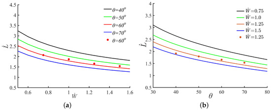
Figure 6. The dependency of the spreading length $\dot{L}$ on (a) the confinement width $\dot{W}$ and (b) wetting angle $\theta$. The solid lines represent the predicted values by Equation (18), and the data points are the numerical results.

Figure 7a,b present the evolution of the spreading length $\dot{L_n}$ and the height $\dot{H_n}$ for different confinement widths $\dot{W}$ at $\theta ={60}^{\circ }$. The dimensionless widths $\dot{W}$ are 0.75, 1.0, 1.25, and 1.5, respectively. It can be seen from Figure 7 that at early times all $\dot{L_n}$ and $\dot{H_n}$ curves coincide with each other because the contact line moves freely before reaching the boundary of the confinement, and the width has no effect on the spreading. Once the contact line reaches the boundary, the contact line is pinned there, and at the same time the spreading is slowed down. Finally, the spreading length $\dot{L_n}$ reaches a limit. Figure 7a shows that a droplet on a wider confinement has a faster spreading speed but takes a shorter time to reach the equilibrium state due to the smaller spreading length $\dot{L_n}$. The height of the droplet oscillates slightly as can be seen in Figure 7b. The amplitude of the oscillations decreases with increasing dimensionless width $\dot{W}$.

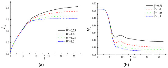
Figure 7. The dependency of confinement width $\dot{W}$ on the evolution of (a) numerical spread length $\dot{L_n}$ and (b) height $\dot{H_n}$ for $\theta ={60}^{\circ }$.

Figure 8a,b show the evolution of the spreading length $\dot{L_n}$ and the height $\dot{H_n}$ and how they depend on the confinement wetting angle $\theta$ for $\dot{W}=1.25$. The wetting angles $\theta$ are ${40}^{\circ }$, ${50}^{\circ }$, ${60}^{\circ }$, ${70}^{\circ }$, respectively. As shown in Figure 8a, the droplet with a lower confinement wetting angle has a higher spreading speed and larger spreading length $\dot{L}$ but takes a longer time to reach the equilibrium state. It is seen in Figure 8b that the height $\dot{H_{max}}$ of a droplet on a lower confinement wetting angle decreases faster, and the oscillation amplitude in the vertical direction increases with a decreasing wetting angle $\theta$.

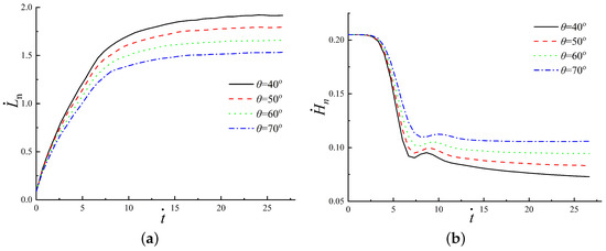
Figure 8. The dependency of wetting angle $\theta$ on the evolution of (a) numerical spread length $\dot{L_n}$ and (b) height $\dot{H_n}$ for confinement width $\dot{W}=1.25$.

3.2.2. Prediction of the Confined Angle

Next, we consider the prediction of the confinement angle ${\theta }^{\ast }$. The volume of the droplet $V_d$ can also be expressed by the integral of the cross-section area $A^{\ast }\left(x\right)$ over the spread length $L^{\ast }$. Using Equation (21), we have

$${\int }_{L^{\ast }}{A}^{\ast }\left(x\right)dx={\int }_{W}A\left(y\right)dy.$$

(26)

As before, the integration is simplified by

$${\int }_{L^{\ast }}{A}^{\ast }\left(x\right)dx=\epsilon L^{\ast }{W}^2{\displaystyle \frac{{\theta }^{\ast }-sin\left({\theta }^{\ast }\right)cos\left({\theta }^{\ast }\right)}{4sin\left({\theta }^{\ast }\right)sin\left({\theta }^{\ast }\right)}}.$$

(27)

By substituting Equations (24) and (27) into (26), the confined angle ${\theta }^{\ast }$ can be expressed as

$${\displaystyle \frac{{\theta }^{\ast }-sin\left({\theta }^{\ast }\right)cos\left({\theta }^{\ast }\right)}{sin\left({\theta }^{\ast }\right)sin\left({\theta }^{\ast }\right)}}={\displaystyle \frac{\dot{L}}{\dot{W}}}{\displaystyle \frac{\theta -sin\left(\theta \right)cos\left(\theta \right)}{sin\left(\theta \right)sin\left(\theta \right)}}.$$

(28)

Equation (28) can be further simplified by substituting Equation (25) into (28), which can be written as

$$\dot{\psi }\left({\theta }^{\ast }\right)=\sqrt{{\displaystyle \frac{2\pi }{3\epsilon {\dot{W}}^3}}\dot{\psi }\left(\theta \right)},$$

(29)

where $\dot{\psi }\left(\theta \right)=(\theta -sin\left(\theta \right)cos\left(\theta \right))/{sin}^2\left(\theta \right)$. It can be seen from Equation (29) that the confinement angle ${\theta }^{\ast }$ can be determined for a given value of the wetting angle $\theta$ of the confinement and the dimensionless width $\dot{W}$.

Figure 9a,b show the predictions of $\dot{\psi }\left({\theta }^{\ast }\right)$ by Equation (29) for different values of $\dot{W}$ and $\dot{\psi }\left(\theta \right)$, respectively. The data points obtained from the numerical simulations agree reasonably well with the corresponding prediction of $\dot{\psi }\left({\theta }^{\ast }\right)$ when the correction factor is $\epsilon =0.8$. Figure 9a shows a decrease in $\dot{\psi }\left({\theta }^{\ast }\right)$ with an increase in the confinement width $\dot{W}$, and that the influence of the width $\dot{W}$ on the variation of $\dot{\psi }\left({\theta }^{\ast }\right)$ becomes weak for large $\dot{W}$. It can be also seen from Figure 9a the discrepancy between the data points and that the prediction curve is increasing with the increasing in $\dot{W}$. This is due to a constant volume correction factor $\epsilon$ being used here as the droplet recovers the spherical cap shape. Figure 9b shows how $\dot{\psi }\left({\theta }^{\ast }\right)$ changes with $\dot{\psi }\left(\theta \right)$ for different confinement widths $\dot{W}$. It is clear that an increase in $\dot{\psi }\left(\theta \right)$ results in an increase in $\dot{\psi }\left({\theta }^{\ast }\right)$.

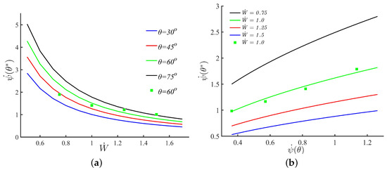
Figure 9. The dependency of $\dot{\psi }\left({\theta }^{\ast }\right)$ on (a) confinement width $\dot{W}$ and (b) $\dot{\psi }\left(\theta \right)$. The solid lines represent the predicted values by Equation (22), and the data points are the numerical results.

In Figure 10a, the evolution of confinement angle ${\theta }^{\ast }$ and the effect of the confinement width $\dot{W}$ for $\theta ={60}^{\circ }$ are demonstrated. The dimensionless widths $\dot{W}$ are 0.75, 1.0, 1.25, and 1.5, respectively. As shown in Figure 10a, decreasing $\dot{W}$ of the confinement results in higher value of the confinement angle ${\theta }^{\ast }$. The ${\theta }^{\ast }$ is higher than ${90}^{\circ }$ when the width $\dot{W}$ decreases to 0.75, which is an undesirable condition for the uniform liquid line. Figure 10b shows the evolution of the confinement angle ${\theta }^{\ast }$ versus the wetting angle $\theta$ for $\dot{W}=1.0$. The values of $\theta$ are ${30}^{\circ }$, ${45}^{\circ }$, ${60}^{\circ }$, ${75}^{\circ }$, respectively. It can be seen that a larger confinement angle ${\theta }^{\ast }$ can be obtained by increasing $\theta$, and that ${\theta }^{\ast }$ is larger than ${90}^{\circ }$ at $\theta ={75}^{\circ }$.

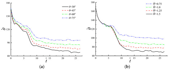
Figure 10. The dependency of the evolution of confinement angle ${\theta }^{\ast }$ on width $\dot{W}$ and wetting angle $\theta$ for (a) $\theta ={60}^{\circ }$ and (b) $\dot{W}=1.0$.

3.3. Formation of Uniform Lines

Simulations of the displacement of sequential droplets in this section in a $10D_0\times 5D_0\times 2.5D_0$ domain resolved by a $200\times 100\times 50$ grid. The shape of a liquid line depends on the spacing $\Delta x$ between each droplet [16]. A large value of $\Delta x$ may cause the liquid line to break apart and form satellite droplets, while a small value of $\Delta x$ can result in a liquid pool. A liquid line is obtained at the predicted droplet spacing $\Delta x$. For a stable and uniform line, the cross-sectional area $A^{\ast }$ and the droplet spacing $\Delta x$ should satisfy

$$\Delta x=V_d/A^{\ast }.$$

(30)

By substituting $A^{\ast }=W^2\dot{\psi }\left({\theta }^{\ast }\right)/4$ into Equation (30) and combining the results with Equation (29), the dimensionless droplet spacing $\Delta \dot{x}$ can be expressed as

$$\Delta \dot{x}=\sqrt{{\displaystyle \frac{2\pi \epsilon }{3\dot{W}\dot{\psi }\left(\theta \right)}}},$$

(31)

where $\Delta \dot{x}=\Delta x/D_0$. It can be seen from Equation (31) that the dimensionless droplet spacing $\Delta \dot{x}$ depends on a given value of the wetting angle $\theta$ of the confinement and the dimensionless width $\dot{W}$.

Figure 11a shows the predicted $\Delta \dot{x}$ as predicted by Equation (31) versus $\theta$. As shown in Figure 11a a droplet on a confinement with a higher wetting angle $\theta$ needs smaller spacing $\Delta \dot{x}$ to form a uniform line. Figure 11b presents the predicted $\Delta \dot{x}$ by Equation (31) versus $\dot{W}$. It can be seen from Figure 11b that the decrease in droplet spacing $\Delta \dot{x}$ results from an increase in the dimensionless width $\dot{W}$.

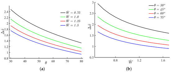
Figure 11. The predicted droplet spacing $\Delta \dot{x}$ for uniform lines for (a) given wetting angle $\theta$ and (b) confinement width $\dot{W}$. The solid lines represent the predicted value by Equation (24).

Figure 12 shows the simulation results for the formation of a uniform liquid line by the displacement of four droplets on a confinement surface. The dimensionless droplet spacing ($\Delta \dot{x}=1.43$) is predicted by Equation (31) for $\dot{W}=1.0$ and $\theta ={60}^{\circ }$. It can be seen from Figure 12 that the four overlapping droplets are displaced, spread, and coalesce with each other and eventually form a uniform liquid line. The contact lines are pinned at the boundaries of the confinement. It is obvious that the liquid line has two parallel contact lines with fixed width, which is the advantageous boundary condition for the uniform line.

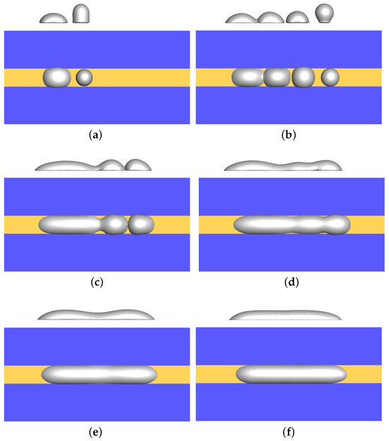
Figure 12. Displacement of sequential droplets by predicted droplet spacing $\Delta \dot{x}=1.43$: (a) $\dot{t}=6.0$; (b) $\dot{t}=13.3$; (c) $\dot{t}=18.0$; (d) $\dot{t}=20.7$; (e) $\dot{t}=30.7$; (f) $\dot{t}=50.0$. Top and bottom are the side view and top view for each panel, respectively.

To investigate the shape evolution and the quality of the line, the cross section error $\zeta$ of the cross-section area $A^{\ast }\left(x\right)$ along the length $L^{\ast }$ of the line (x direction) is utilized to quantify the uniformity. The $\zeta$ is defined by

$$\zeta =\sqrt{{\displaystyle \frac{\int {(A^{\ast }\left(x\right)-\overline{A})}^{2}dx}{L^{\ast }}}},$$

(32)

where $\overline{A}$ is the average cross-section area.

In the numerical computation, the value of the index function is utilized to calculate the $\zeta$, and Equation (32) is approximated by

$$\zeta =\sqrt{{\displaystyle \frac{{\sum }_{i=i_1}^{i_2}{(I\left(i\right)-\overline{I})}^2}{i_2-i_1+1}}},$$

(33)

where $i_1$ and $i_2$ are the front and rear end grid points of the liquid line, $I\left(i\right)$ is the index value at grid point i, and $\overline{I}$ is the average index value. Here, we take a value of 1 inside the droplet and 0 in the ambient.

Figure 13a,b show the liquid lines at $\dot{t}=50.0$ formed by alternative droplet spacing, $\Delta \dot{x}=1.1$ in (a) and $\Delta \dot{x}=1.6$ in (b). The time is the same as the last time in Figure 12. In each frame, the top shows the line from the side and the bottom shows the line from above. In Figure 13a, where $\Delta \dot{x}$ is smaller than the predicted value, the line has a big hump in the middle, although its width is relatively uniform. When $\Delta \dot{x}$ is larger than the predicted value, the line has a depression in the middle and a slight neck near one end, when viewed from above. Thus, at the time shown, the lines are less uniform than the line formed using the predicted spacing. To quantify how the shape of the line evolves with time, we plot the $\zeta$ versus time in Figure 14 for the three cases shown in Figure 12 and Figure 13. The solid line is the optimum spacing and we see that the non-uniformity drops relatively quickly and is roughly uniform after about time 25 to 30. The uniformity decays slightly slower for $\Delta \dot{x}$ less than the optimum value, although eventually it is comparable with what we see for the optimum value. For $\Delta \dot{x}$ larger than the optimum value, the $\zeta$ first decreases but not to the same value as for the optimum $\Delta \dot{x}$, and then increases, suggesting that the line may be splitting into separate droplets.

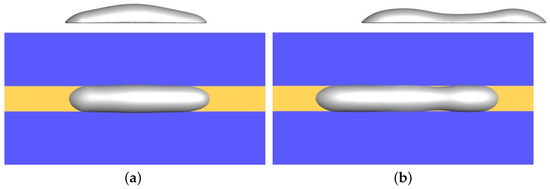
Figure 13. Liquid lines formed by alternative droplet spacing: (a) $\Delta \dot{x}=1.1$; (b) $\Delta \dot{x}=1.6$.

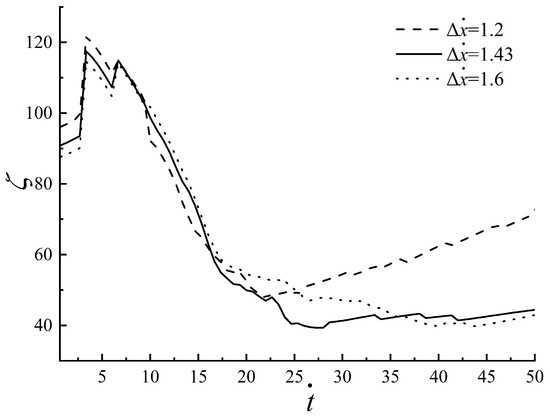
Figure 14. Evolution of the uniformity $\zeta$ as a function of time for different droplet spacing $\Delta \dot{x}$.

4. Conclusions

The numerical model based on FTM is developed to investigate the droplet displacement mechanism on a wetting confinement. An analytical model is derived to predict the droplet spacing for the formation of a liquid line on a wetting confinement, the evolution of the droplet’s morphology and the formation of a uniform line is simulated numerically. The main conclusions are as follows:

(1)

The spreading length $\dot{L_n}$ and the function $\dot{\psi }\left({\theta }^{\ast }\right)$ found by the numerical simulations align well with the corresponding analytic prediction when the volume correction factor $\epsilon$ is taken as 0.8.

(2)

The evolution of the spreading $\dot{L}$ shows that in the early stages of the displacement, the width $\dot{W}$ of the confinement has no effect on the spreading, due to the free movement of the contact line before it reaches the boundary of the confinement. In addition, the dimensionless width $\dot{W}$ and the wetting angle $\theta$ have a significant impact on the amplitude of the oscillations in the vertical direction.

(3)

The pinned contact line on the boundaries of the confinement are parallel. With a droplet spacing $\Delta \dot{x}$, predicted by Equation (31), it is feasible to form a liquid line with a lower cross-section area and higher uniformity by the sequential displacement of droplets on the wetting confinement.

References

- Samusjew, A.; Kratzer, M.; Moser, A.; Teichert, C.; Krawczyk, K.K.; Griesser, T. Inkjet printing of soft, stretchable optical waveguides through the photopolymerization of high-profile linear patterns. ACS Appl. Mater. Interfaces 2017, 9, 4941–4947. [Google Scholar] [CrossRef]
- Hamad, A.; Mian, A.; Khondaker, S.I. Direct-write inkjet printing of nanosilver ink (UTDAg) on peek substrate. J. Manuf. Processes 2020, 55, 326–334. [Google Scholar] [CrossRef]
- Rajashekhar, V.S.; Pravin, T.; Thiruppathi, K. A review on droplet deposition manufacturing a rapid prototyping technique. Int. J. Manuf. Technol. Manag. 2019, 33, 362–383. [Google Scholar] [CrossRef]
- Khoo, H.; Allen, W.S.; Arroyo-Currás, N.; Hur, S.C. Rapid prototyping of thermoplastic microfluidic devices via SLA 3D printing. Sci. Rep. 2024, 14, 17646. [Google Scholar] [CrossRef] [PubMed]
- Qi, L.; Zhong, S.; Luo, J.; Zhang, D.; Zuo, H. Quantitative characterization and influence of parameters on surface topography in metal micro-droplet deposition manufacture. Int. J. Mach. Tools Manuf. 2015, 88, 206–213. [Google Scholar] [CrossRef]
- Ma, Y.; Wang, S.; Wu, Z. Photolithographic Microfabrication of Microbatteries for On-Chip Energy Storage. Nano-Micro Letters. 2025, 17, 105. [Google Scholar] [CrossRef]
- Jung, H.C.; Cho, S.H.; Joung, J.W.; OH, Y.S. Studies on Inkjet-Printed Conducting Lines for Electronic Devices. J. Electron. Mater. 2007, 36, 1211–1218. [Google Scholar] [CrossRef]
- Kastner, J.; Faury, T.; Aurberhuber, H.M. Silver-based reactive ink for inkjet-printing of conductive lines on textiles. J. Electron. Mater. 2017, 176, 84–88. [Google Scholar] [CrossRef]
- Graham, P.J.; Farhangi, M.M.; Dolatabadi, A. Dynamics of droplet coalescence in response to increasing hydrophobicity. Phys. Fluids 2012, 24, 112105. [Google Scholar] [CrossRef]
- Zhang, L.; Zhu, Y.; Cheng, X. Numerical investigation of multi-droplets deposited lines morphology with a multiple-relaxation-time Lattice Boltzmann model. Chem. Eng. Sci. 2017, 171, 534–544. [Google Scholar] [CrossRef]
- Dalili, A.; Chandra, S.; Mostaghimi, J.; Charles Fan, H.T.; Simmer, J.C. Formation of liquid sheets by deposition of droplets on a surface. J. Colloid Interface Sci. 2014, 418, 292–299. [Google Scholar] [CrossRef] [PubMed]
- Singh, J.; Roy, S. Coalescence preference dynamics for droplet growth during single-component fluid phase separation. Front. Phys. 2022, 10, 1027192. [Google Scholar] [CrossRef]
- Du, Z.; Xing, R.; Cao, X.; Yu, X.; Han, Y. Symmetric and uniform coalescence of ink-jetting printed polyfluorene ink drops by controlling the droplet spacing distance and ink surface tension/viscosity ratio. Polymer 2017, 115, 45–51. [Google Scholar] [CrossRef]
- Davis, S.H. Moving Contact Lines and Rivulet Instabilities-1. The Static Rivulet. J. Fluid Mech. 1980, 98, 225–242. [Google Scholar]
- Schiaffino, S.; Sonin, A.A. Formation and stability of liquid and molten beads on a solid surface. J. Fluid Mech. 1997, 343, 95–110. [Google Scholar] [CrossRef]
- Duineveld, P.C. The stability of ink-jet printed lines of liquid with zero receding contact angle on a homogeneous substrate. J. Fluid Mech. 2003, 447, 175–200. [Google Scholar] [CrossRef]
- Thompson, A.B.; Tipton, C.R.; Juel, A.; Hazel, A.L.; Dowling, M. Sequential deposition of overlapping droplets to form a liquid line. J. Fluid Mech. 2014, 761, 261–281. [Google Scholar] [CrossRef]
- Cheng, X.; Zhu, Y.; Zhang, L.; Wang, C.; Li, S. Lattice Boltzmann simulation of multiple droplets impingement and coalescence in an inkjet-printed line patterning process. Int. J. Comput. Fluid Dyn. 2017, 31, 450–462. [Google Scholar] [CrossRef]
- Cheng, X.; Zhu, Y.; Zhang, L.; Zhang, D.; Ku, T. Numerical analysis of deposition frequency for successive droplets coalescence dynamics. Phys. Fluids 2018, 30, 042102. [Google Scholar] [CrossRef]
- Stringer, J.; Derby, B. Formation and Stability of Lines Produced by Inkjet Printing. Langmuir 2010, 26, 10365–10372. [Google Scholar] [CrossRef]
- Soltman, D.; Subramanian, V. Inkjet-Printed Line Morphologies and Temperature Control of the Coffee Ring Effect. Langmuir 2008, 24, 2224–2231. [Google Scholar] [CrossRef] [PubMed]
- Abunahla, R.; Rahman, M.S.; Naderi, P. Improved Inkjet-Printed Pattern Fidelity: Suppressing Bulges by Segmented and Symmetric Drop Placement. J. Micro- Nano-Manuf. 2020, 8, 031001–031002. [Google Scholar] [CrossRef]
- Ma, C.; Bothe, D. Direct numerical simulation of thermocapillary flow based on the volume of fluid method. Int. J. Multiph. Flow 2011, 37, 1045–1058. [Google Scholar] [CrossRef]
- Popinet, S. An accurate adaptive solver for surface-tension-driven interfacial flows. J. Comput. Phys. 2009, 228, 5838–5866. [Google Scholar] [CrossRef]
- Aland, S.; Voigt, A. Benchmark computations of diffuse interface models for two-dimensional bubble dynamics. Int. J. Numer. Methods Fluids 2012, 69, 747–761. [Google Scholar] [CrossRef]
- Frachon, T.; Zahedi, S. A cut finite element method for incompressible two-phase Navier–Stokes flows. J. Comput. Phys. 2019, 384, 77–98. [Google Scholar] [CrossRef]
- Agnese, M.; Nürnberg, R. Fitted front tracking methods for two-phase incompressible Navier–Stokes flow: Eulerian and ALE finite element discretizations. Int. J. Numer. Anal. Mod. 2020, 17, 613–642. [Google Scholar]
- Duan, B.; Li, B.; Yang, Z. An energy diminishing arbitrary Lagrangian–Eulerian finite element method for two-phase Navier–Stokes flow. J. Comput. Phys. 2022, 461, 111215. [Google Scholar] [CrossRef]
- Inguva, V.; Kenig, E.Y.; Perot, J.B. A front-tracking method for two-phase flow simulation with no spurious currents. J. Comput. Phys. 2022, 456, 111006. [Google Scholar] [CrossRef]
- Pan, J.; Long, T.; Chirco, L.; Scardovelli, R.; Popinet, S.; Zaleski, S. An edge-based interface tracking (EBIT) method for multiphase-flow simulation with surface tension. J. Comput. Phys. 2024, 508, 113016. [Google Scholar] [CrossRef]
- Wang, Z.; Chen, E.; Zhao, Y. The effect of surface anisotropy on contact angles and the characterization of elliptical cap droplets. Sci. China Technol. Sci. 2018, 61, 309–316. [Google Scholar] [CrossRef]
- Peskin, C.S. Numerical analysis of blood flow in the heart. J. Comput. Phys. 1997, 25, 220–252. [Google Scholar] [CrossRef]
- Tryggvason, G.; Scardovelli, R.; Zaleski, S. Direct Numerical Simulations of Gas-Liquid Multiphase Flows; Cambridge University Press: Cambridge, UK, 2011. [Google Scholar]
- Zhang, H.; Liu, L.; Liao, Y.; Tan, Z.; Yan, H. Numerical simulation on bubble deformation and forces at moderate Reynolds number using front-tracking algorithm coupled with proportional-integral-derivative controller. Phys. Fluids 2024, 36, 113303. [Google Scholar] [CrossRef]
- Zhu, G.; Kou, J.; Yao, B.; Wu, Y.S.; Yao, J.; Sun, S. Thermodynamically consistent modelling of two-phase flows with moving contact line and soluble surfactants. J. Fluid Mech. 2019, 879, 327–359. [Google Scholar] [CrossRef]
- Zhu, G.; Kou, J.; Yao, J.; Li, A.; Sun, S. A phase-field moving contact line model with soluble surfactants. J. Comput. Phys. 2020, 405, 109170. [Google Scholar] [CrossRef]
- Li, W.; Lu, J.; Tryggvason, G.; Zhang, Y. Numerical study of droplet motion on discontinuous wetting gradient surface with rough strip. Phys. Fluids 2021, 33, 012111. [Google Scholar] [CrossRef]
- Gao, F.; Sonin, A.A. Precise deposition of molten microdrops: The physics of digital microfabrication. Proc. R. Soc. A 1994, 444, 533–554. [Google Scholar]
Disclaimer/Publisher’s Note: The statements, opinions and data contained in all publications are solely those of the individual author(s) and contributor(s) and not of MDPI and/or the editor(s). MDPI and/or the editor(s) disclaim responsibility for any injury to people or property resulting from any ideas, methods, instructions or products referred to in the content. |
© 2025 by the authors. Licensee MDPI, Basel, Switzerland. This article is an open access article distributed under the terms and conditions of the Creative Commons Attribution (CC BY) license (https://creativecommons.org/licenses/by/4.0/).