Adaptive Structured Latent Space Learning via Component-Aware Triplet Convolutional Autoencoder for Fault Diagnosis in Ship Oil Purifiers

Abstract

Timely and accurate fault diagnosis of ship oil purifiers is essential for maintaining the operational reliability of a degree-4 maritime autonomous surface ship (MASS). Conventional approaches rely on manual feature engineering or simple machine learning classifiers, limiting their robustness in dynamic maritime environments. This study proposes an adaptive latent space learning framework that couples a two-dimensional convolutional autoencoder (2D-CAE) with a component-aware triplet-loss regularizer. The loss term structures the latent space to reflect both the fault severity progression and component-specific distinctions, enabling severity-proportional distances among a latent vector learned directly from vibration signals even in a limited data environment. Using data collected on a dedicated ship oil purifier test bed, the method yields a latent vector that encodes the fault severity and physical provenance, enhancing the interpretability and diagnostic accuracy. Experiments demonstrate enhanced performance over state-of-the-art deep models, while offering clear insight into fault evolution and inter-component dependencies. The framework thus advances intelligent, condition-based maintenance for autonomous maritime systems.

1. Introduction

The maritime sector is rapidly adopting maritime autonomous surface ships, with degree-4 vessels capable of operating without human intervention. These autonomous ships promise to transform global shipping through improved efficiency, sustainability, and safety [1]. However, their success depends on exceptional operational reliability. Without onboard crew, minor defects can quickly escalate into mission-critical failures, making continuous self-diagnosis and health monitoring essential [2].

Within this autonomous ecosystem, the dependable functioning of auxiliary subsystems is intrinsically related to the vessel’s overall integrity. Ship oil purifiers, which are centrifugal separators tasked with excising deleterious water, sludge, and metallic particulates from fuel and lubricating oils, constitute a particularly critical subsystem [3,4]. Inadequate purification often stems from mechanical degradation, where faults such as bearing wear, mass imbalance from sludge, and drive system defects manifest as distinct changes in the machine’s vibration signature [5], causing accelerated engine wear, diminished power generation, and compromised safety margins, thereby jeopardizing both the propulsion and electrical power trains [3,6]. Consequently, the construction of diagnostic methodologies that reliably, accurately, and promptly detect purifier faults is indispensable to the viability of autonomous maritime operations.

Historically, purifier fault diagnosis has been formulated as a two-stage procedure encompassing, first, the derivation of discriminative features from raw sensor streams (typically vibration signals) and, second, the classification of health states based on those features [7]. In practice, fluctuating loads and stochastic sea states make manual feature design difficult. Conventional approaches, predicated on domain experts selecting statistical or spectral descriptors, frequently exhibit insensitivity to incipient faults and dependence on heuristic judgment, thereby demonstrating insufficient performance under the nonlinear, non-stationary dynamics prevalent in situ [8]; moreover, they seldom exploit the rich inter-channel couplings that emerge when multiple accelerometers are deployed.

In contrast, data-driven paradigms that leverage deep learning have demonstrated appreciable capability for adaptive feature extraction and nonlinear representation [9,10]. Architectures such as one-dimensional convolutional neural networks (1D-CNNs) and classical autoencoders have already been utilized to infer latent health information directly from raw vibration data. Nevertheless, because 1D kernels process each sensor channel independently, they generally fail to capture the cross-channel dynamics that precede mechanical degradation. Two-dimensional convolutional models, which conceptualize the multi-channel time series as an image-like tensor, overcome this limitation by learning joint spatio-temporal patterns and, when combined with channel attention mechanisms, by weighting sensor streams according to their diagnostic salience [11]. Beyond general-purpose designs, maritime-focused studies have recently broadened this landscape: autoencoder-based anomaly detection with the Mahalanobis distance deployed within an integrated digital-twin decision platform for induction motor monitoring [12], frameworks that augment scarce data of diesel generator failure modes [13], data-driven fault-tolerant control of ship power–condenser systems via real-time optimization [14], and ”agentic” large language model-assisted anomaly-reasoning pipelines that contextualize multimodal signals across shipping operations [15]. However, combined with agentic or spatio-temporal pattern learning methods, complex deep learning algorithms require a large amount of training data for high performance.

Metric learning, notably triplet-loss, further structures the latent space and helps in limited-data settings. Triplet-loss optimizes the latent vector such that anchor–positive pairs (from the same class) are closer than anchor–negative pairs (from different classes), thereby enhancing intra-class cohesion and inter-class separability, even under a limited-data environment [16]. However, the canonical formulation remains class-centric: it neither imposes an ordinal structure reflecting fault-severity progression nor acknowledges functional distinctions between faults arising in disparate machine components. Adaptive margin triplet-loss has recently been proposed to modulate the margin according to relative ratings and can improve the training stability and ranking performance [17]. Triplet-loss has also been used to guide adversarial domain adaptation for bearing fault diagnosis, where it aligns class-level distributions across domains and improves transferability [18]. Yet, to fully harness these metric-learning advancements within an MASS, diagnostic frameworks must extend beyond mere classification and explicitly represent both the severity gradations and the distinct origins of faults across ship subsystems.

To address these deficiencies, the present study proposes an adaptive structured latent-space learning framework for ship oil purifier fault diagnosis, denoted as AS-LSLF hereinafter. The framework integrates a two-dimensional convolutional autoencoder (2D-CAE) augmented with lightweight channel-attention blocks and a component-aware triplet-loss function. By actively arranging the latent manifold, the proposed loss ensures that the latent vector simultaneously encodes (i) ordinal fault-severity levels so that degradation levels appear proportionally spaced and (ii) categorical distinctions between physical subsystems, such as the bowl assembly versus the drive train. This design yields discriminative, interpretable features from raw vibration data, improving the diagnostic accuracy and insight into fault evolution. The principal contributions of this work are threefold:

• We construct an automated latent-space learning framework that couples a channel-attentive 2D-CAE with a metric-learning objective, thereby obviating manual feature engineering and yielding interpretable latent vector from six-channel vibration signals.
• We introduce a component-aware triplet-loss formulation that jointly embeds ordinal severity information and categorical component identity, enhancing robustness and explanatory power in the resulting diagnostic model.
• We validate the proposed framework on a dedicated ship oil purifier test bed, demonstrating superior accuracy and interpretability relative to conventional feature fusion methods and contemporary deep learning baselines.

Section 2 delineates the architecture of the adaptive structured latent-space learning framework, details the component-aware triplet-loss formulation, and presents the experimental environment, simulated fault conditions, and data acquisition protocol. Section 3 analyses the empirical results, comparing the proposed approach with benchmark models and examining the learned latent structure. Finally, Section 4 summarizes the principal findings and discusses their implications for condition-based maintenance in autonomous maritime systems.

2. Methodology: Adaptive Structured Latent-Space Learning Framework

2.1. Proposed Framework and Problem Formulation

Conventional deep learning pipelines for machinery diagnosis frequently regard feature extraction as an opaque optimization exercise driven exclusively by classification accuracy. These black-box representations, although occasionally effective under stationary conditions, generally deteriorate when confronted with limited training data, showing limited explanatory power for maintenance personnel and, of particular consequence for degree-4 MASSs, provide no principled mechanism for monitoring fault progression. To address this limitation, the present study proposes an adaptive structured latent space learning framework that couples a two-dimensional convolutional autoencoder 2D-CAE with a component-aware, severity-preserving metric-learning scheme augmented by lightweight channel attention modules. The framework (i) uses raw six-channel vibration data from multiple subsystems; (ii) organizes the latent manifold so the latent vector encodes location and severity; and (iii) produces a compact, interpretable latent vector for downstream diagnosis or prognosis.

Figure 1 summarizes the operational flow and principal constituents of the proposed architecture, where raw six-channel vibration snippets are encoded by a 2D-CAE; the encoder is trained with a composite loss that enforces reconstruction fidelity, component-wise separability, and severity-wise ordering. The resulting latent vectors subsequently drive a lightweight classifier for real-time fault-type and severity recognition. The remainder of this section is structured as follows: Section 2.2 delineates the 2D-CAE architecture and attendant receptive-field design; Section 2.3 shows the composite loss function and articulates the triplet-sampling logistics and describes the downstream classifier, together with the adopted training regimen. Collectively, these modules establish a methodological foundation for the experimental validation presented in Section 3.

2.2. Two-Dimensional Convolutional Autoencoder

After being first proposed by LeCun et al. [19] for image classification, convolutional neural networks (CNNs) have been widely used to analyze raw data for feature learning and have shown promise in automatically extracting relevant features from complex sensor data. By leveraging the hierarchical learning capabilities of CNNs, we aim to enhance the feature extraction process within our proposed framework by utilizing the CAE structure. A conventional AE is generally composed of two components, corresponding to the encoder $f(·)$ and decoder $f^{\prime }(·)$. It aims to find parameters for reconstructing the original input data by optimizing the AE parameter ($\theta$), and thus, minimizing the mean squared errors (MSEs) between the input and reconstructed output over all samples.

$$\underset{\theta }{min}{\displaystyle \frac{1}{n}}\sum _{i=1}^n{∥f^{\prime }\left(f\left({\mathbf{x}}_i\right)\right)-{\mathbf{x}}_i∥}_2^2$$

(1)

To leverage the spatial organization of the input-exemplified by multivariate time-series sensor measurements from a ship oil purifier, we employ a convolutional autoencoder. A CAE integrates local convolutional connectivity within the autoencoder framework to learn compact, structure-aware representations. The forward transformation that maps inputs to latent feature maps is the convolutional encoder, while the inverse operation that reconstructs the outputs via deconvolution constitutes the convolutional decoder [20].

The CAE mirrors a conventional autoencoder, where $f(·)$ denotes the convolutional encoding operation and $f^{\prime }(·)$ denotes the convolutional decoding operation. Let the input feature maps be $\mathbf{x}\in {\mathbb{R}}^{n\times l\times l}$, produced either by the input layer or by the preceding layer, comprising n maps, each of spatial size $l\times l$. The layer employs m convolutional kernels, and therefore, yields m output feature maps. If the maps originate from the input layer, n equals the number of input channels; otherwise, n equals the number of output feature maps produced by the previous layer. Each convolutional kernel has size $d\times d$ with $d\le l$.

$\theta =\mathbf{W},\widehat{\mathbf{W}},\mathbf{b},\widehat{\mathbf{b}}$ collects the learnable parameters of a CAE layer, where $\mathbf{b}\in {\mathbb{R}}^m$ and $\mathbf{W}={\mathbf{w}}_j$, $j=1,2,\dots ,m$, correspond to the convolutional encoder, with ${\mathbf{w}}_j\in {\mathbb{R}}^{n\times d\times d}$ (and, when flattened, ${\mathbf{w}}_j\in {\mathbb{R}}^{n{d}^2}$). Analogously, the decoder is parameterized by $\widehat{\mathbf{W}}={\widehat{\mathbf{w}}}_j$, $j=1,2,\dots ,m$, and $\widehat{\mathbf{b}}$, with $\widehat{\mathbf{b}}\in {\mathbb{R}}^n$ and ${\widehat{\mathbf{w}}}_j\in {\mathbb{R}}^{1\times n{d}^2}$.

Encoding proceeds by sliding a $d\times d$ patch ${\mathbf{x}}_i$, $i=1,2,\dots ,p$, across the input and convolving it with the weight ${\mathbf{w}}_j$ of the j-th kernel, after which the output neuron values $o_{ij}$, $j=1,2,\dots ,m$, are computed at the layer output. Within each convolutional layer, kernels impose local receptive fields and sparse inter-layer connectivity, enabling detectors that capture spatially localized patterns. Through successive convolutions, these detectors reorganize information so that feature maps with similar statistics become aligned, and the layer implements the following mapping:

$$o_{ij}=\phi \left(\sum _{k=1}^n{\mathbf{x}}_i^k\ast {\mathbf{w}}_j^k+b_j\right),$$

(2)

where ${\mathbf{x}}_i^k$ is the k-th channel of the input patch, ${\mathbf{w}}_j^k$ is the weight for channel k in kernel j, and $b_j$ is the bias for the j-th output map; $\phi$ denotes an activation function such as $\mathrm{Sigmoid}\left(x\right)=1/(1+e^{-x})$ or $\mathrm{ReLU}\left(x\right)=max(0,x)$.

To compress the spatial resolution and impart invariance to small local perturbations, pooling layers are inserted after one or more convolutions in the CAE. In this study, max-pooling is adopted and defined as

$$o_j^{m+1}(c,d)=\underset{0\le p,q<r}{max}{o}_j^m(c·r+p,d·r+q),$$

(3)

where $o_j^m$ is the j-th feature map at layer m, $o_j^{m+1}(c,d)$ is the pooled element at coordinates $(c,d)$ of layer $m+1$, r is the pooling window size, and p and q are the index positions within the corresponding local region of the input.

After traversing the convolutional and pooling stages, the feature maps produced by the final convolutional block are vectorized and concatenated into a single representation:

$${\mathbf{z}}_{\mathrm{flatten}}=\mathrm{flatten}\left({\mathbf{o}}^{m+1}\right),$$

(4)

where ${\mathbf{o}}^{m+1}$ denotes the collection of output maps from the encoder’s last pooling layer $(m+1)$ and ${\mathbf{z}}_{\mathrm{flatten}}$ is the resulting flattened latent vector for downstream processing.

Reconstruction fidelity alone is insufficient for diagnostic separability; hence, the encoder is trained jointly with component-aware and severity-aware triplet-loss introduced in the next subsection, which impose a physically meaningful geometry on the latent space while retaining the reconstruction guarantee. By incorporating this structure, the framework achieves robust feature learning under data scarcity and markedly improves its capacity to extract meaningful representations from complex multi-sensor vibration data.

2.3. Composite Loss for Structured Latent-Space Engineering

The composite loss described in this section formulates a latent space that incorporates not only reconstruction loss but also encodes the locations of faults and the intensity of degradation through triplet-loss, defined as follows: given an anchor sample ${\mathbf{x}}^a$, a positive sample ${\mathbf{x}}^p$ that shares the anchor’s label, and a negative sample ${\mathbf{x}}^n$ drawn from a different label, the network is trained to satisfy

$$\parallel f\left({\mathbf{x}}^a\right)-f\left({\mathbf{x}}^p\right){\parallel }_2^2+\alpha <{\parallel f\left({\mathbf{x}}^a\right)-f\left({\mathbf{x}}^n\right)\parallel }_2^2,$$

(5)

so that the hinge loss

$${\mathcal{L}}_{\mathrm{triplet}}=max\left(D(f\left({\mathbf{x}}^a\right),f\left({\mathbf{x}}^p\right))-D(f\left({\mathbf{x}}^a\right),f\left({\mathbf{x}}^n\right))+\alpha ,0\right),$$

(6)

where $f(·)$ represents the shared CAE encoder, and ${\parallel ·\parallel }_2$ denotes the Euclidean norm, with $D({\mathbf{z}}_1,{\mathbf{z}}_2)={\parallel {\mathbf{z}}_1-{\mathbf{z}}_2\parallel }_2^2$ vanishing only when the margin $\alpha >0$ is respected. In practice, the optimizer receives gradient signals solely from semi-hard and hard triplets—respectively, those satisfying $D(a,p)<D(a,n)<D(a,p)+\alpha$ and $D(a,n)<D(a,p)$—which is a mining strategy that generally accelerates convergence.

To embed distinct aspects of the fault domain, two specialized triplet branches are superimposed upon the reconstruction error ${\mathcal{L}}_{\mathrm{recon}}$. The overall loss reads

$${\mathcal{L}}_{\mathrm{total}}=W_{\mathrm{recon}}{\mathcal{L}}_{\mathrm{recon}}+W_{\mathrm{comp}}{\mathcal{L}}_{\mathrm{comp}}+W_{\mathrm{sev}}{\mathcal{L}}_{\mathrm{sev}},$$

(7)

where $W_{\mathrm{recon}},W_{\mathrm{comp}},W_{\mathrm{sev}}>0$ are trade-off coefficients. The component-aware term operates on triplets $({\mathbf{x}}^a,{\mathbf{x}}^p,{\mathbf{x}}_{\mathrm{comp}}^n)$ selected such that the anchor–positive pair originates from the same physical subsystem and the negative from a different subsystem; employing batch-hard mining [17], the loss

$${\mathcal{L}}_{\mathrm{comp}}=max\left(D(f\left({\mathbf{x}}^a\right),f\left({\mathbf{x}}^p\right))-D(f\left({\mathbf{x}}^a\right),f\left({\mathbf{x}}_{\mathrm{comp}}^n\right))+{\alpha }_{\mathrm{comp}},0\right)$$

(8)

drives inter-component separation. In contrast, the severity-aware branch acts within each component cluster: given a severity level s for both the anchor and positive and a higher-level $s^{\prime }>s$ for the negative ${\mathbf{x}}_{\mathrm{sev}}^n$, we adopt the adaptive margin scheme so that

$${\mathcal{L}}_{\mathrm{sev}}=max\left(D(f\left({\mathbf{x}}^a\right),f\left({\mathbf{x}}^p\right))-D(f\left({\mathbf{x}}^a\right),f\left({\mathbf{x}}_{\mathrm{sev}}^n\right))+{\alpha }_{\mathrm{sev}}\mathsf{\Delta }s,0\right),\mathsf{\Delta }s=s^{\prime }-s,$$

(9)

thereby imposing a monotone ordering whose geodesic length correlates with physical wear.

Figure 2 depicts the geometric effect: (a) demonstrates how the component margin ${\alpha }_{\mathrm{comp}}$ creates well-separated islands, whereas panel (b) illustrates the severity margin ${\alpha }_{\mathrm{sev}}\mathsf{\Delta }s$, which increases linearly with the degradation level, and thus, yields a smoothly ordered trajectory.

Upon convergence, the latent representation $\mathbf{z}=f\left(\mathbf{x}\right)$ is dispatched to two lightweight prediction heads that remain jointly trainable with the 2D-CAE encoder: a softmax classifier delivering component probabilities and a single-neuron sigmoid regressor outputting a continuous severity index. Their cross-entropy and mean squared error contributions enter the composite loss with negligibly small weights so as not to distort the metric-learning geometry.

2.4. Data Description

This subsection describes the protocol for building a high-fidelity vibration dataset under controlled lab conditions. Specifically, a purpose-built, land-based test bed, whose salient features are illustrated in Figure 3, houses an Alfa Laval S805 (Lund, Sweden) centrifugal oil purifier, a unit that is widely deployed across maritime platforms. A three-phase, 3600 rpm (60 Hz) electric motor actuates the purifier’s bowl assembly, which, in turn, attains 9300 rpm through a flat-belt transmission, thereby generating the requisite centrifugal field for contaminant separation. A complementary schematic of the principal subsystems is presented in Figure 4.

The test bed was extensively instrumented to capture dynamic responses representative of disparate health states. Consistent with prior investigations [21], preliminary screening confirmed that broadband vibration is the most sensitive observable for incipient mechanical defects; hence, vibration was selected as the primary diagnostic modality. Two high-sensitivity, tri-axial accelerometers (PCB Piezotronics 356A15 (Depew, NY, USA)) were affixed to the upper frames of the bowl assembly and the drive motor, and their outputs were sampled at 25.6 kHz, a rate that generally affords sufficient bandwidth to resolve fault-induced spectral content.

To emulate realistic failure scenarios, we modeled one baseline and six fault modes, each built at multiple severity levels (

Table 1. Simulated fault conditions and severity definitions.

Component	Fault Mode	Failure Mechanism	Severity Definition
Bowl Assembly	Seal Degradation	Thermal aging hardens and cracks bowl seals, causing leakage and imbalance.	25%: aged at 120 °C for 45 h
			50%: aged at 120 °C for 90 h
			75%: aged at 120 °C for 125 h
			100%: aged at 120 °C for 180 h
	Mass Imbalance	Uneven mass distribution from sludge or wear induces excessive vibration.	25%: 10 g mass attached
			50%: 20 g mass attached
			75%: 30 g mass attached
			100%: 40 g mass attached
Drive System	Bearing Lubrication Fault	Insufficient lubricant in motor bearings increases friction and wear.	Lubricant removed (100%)
	Belt Tension Degradation	Fatigue or stretching of the flat belt causes slippage and power loss.	25%: center distance 82.56 mm
			50%: 80.29 mm
			75%: 78.02 mm
			100%: 75.75 mm
	Friction-Coupling Wear	Progressive loss of elastomer in the flexible coupling increases backlash and torsional resonance.	25%: residual mass 22.21 g
			50%: 14.74 g
			75%: 7.37 g
			100%: 0 g
	Shaft Misalignment	Angular misalignment between the motor shaft and purifier spindle induces bending stress.	25%: shaft tilted by 0.3°
			50%: 0.6°
Normal Condition		All components operating within nominal specifications.

). For each class, the purifier operated for 30 min to attain thermal equilibrium, after which the final 20 min of continuous data were retained. The resulting stream was segmented into 10 s sliding windows with a 1 s overlap. Consequently, every sample constitutes a six-channel time series of length 256,000 (6 channels × 256,000 time steps), corresponding to the x-, y-, and z-axes of the two accelerometers.

3. Results and Discussion

3.1. Experimental Results

To validate the efficacy of the proposed structured latent-space learning approach, an ablation study was conducted. This study compared the full framework (AS-LSLF) with a baseline two-dimensional convolutional autoencoder (2D-CAE) trained only with the standard reconstruction loss, combined with a classification network for both component and severity classifications. The experiments were performed on a PC with an Intel Core Ultra 7265 K processor (Santa Clara, CA, USA), 128 GB of RAM, and an NVIDIA RTX 5090 GPU (Santa Clara, CA, USA). This setup used Python 3.11 (Wilmington, DE, USA) and Pytorch 2.8.0 (New York City, NY, USA) to facilitate the best utilization of the latest software capabilities and GPU acceleration. The hyper-parameters for each model were optimized using grid search optimization. The hyper-parameters for grid search optimization included the learning rate, the number of layers, filter sizes, and regularization terms, as shown in

Table 2. Search ranges used for grid search optimization of the component-aware triplet (2D-CAE) and models for comparison.

Parameter	Range/Options	Purpose in the Code
Latent dimension size	{128, 256, 512}	Width of the bottleneck vector z produced by the encoder.
Learning rate	$[1\times {10}^{-4},5\times {10}^{-3}]$	Initial step size for the Adam optimizer.
Weight decay (L2)	$[1\times {10}^{-6},1\times {10}^{-3}]$	L2 regularization applied by Adam.
Reconstruction weight	$[0.5,2.0]$	Weight of the MSE reconstruction term.
Component triplet weight	$[0.5,2.0]$	Weight of the class-aware triplet-loss on z.
Severity triplet weight	$[0.1,1.0]$	Weight of the continuous-severity triplet-loss.
Triplet margin	$[0.5,2.0]$	Margin used when computing $L_{\mathrm{triplet}\_\mathrm{comp}}$.
Classification weight	$[0.05,1.0]$	Multiplier for the cross-entropy loss on component logits.

. Following this search, the optimal parameters for the final model were a latent dimension size of 256, a learning rate of $5\times {10}^{-4}$, a weight decay of $1\times {10}^{-5}$, a reconstruction weight of $1.0$, a component triplet weight of $1.0$, a severity triplet weight of $0.5$, a triplet margin of $0.8$, and a classification weight of $0.2$. The models were trained for a maximum of 50 epochs, with a batch size of 16. To prevent overfitting and determine the optimal training duration, an early stopping mechanism was employed with a patience of 7 epochs, monitoring the validation loss. The dataset was shuffled and split into a 70:30 train–test split and was stratified to maintain class proportions across all sets. 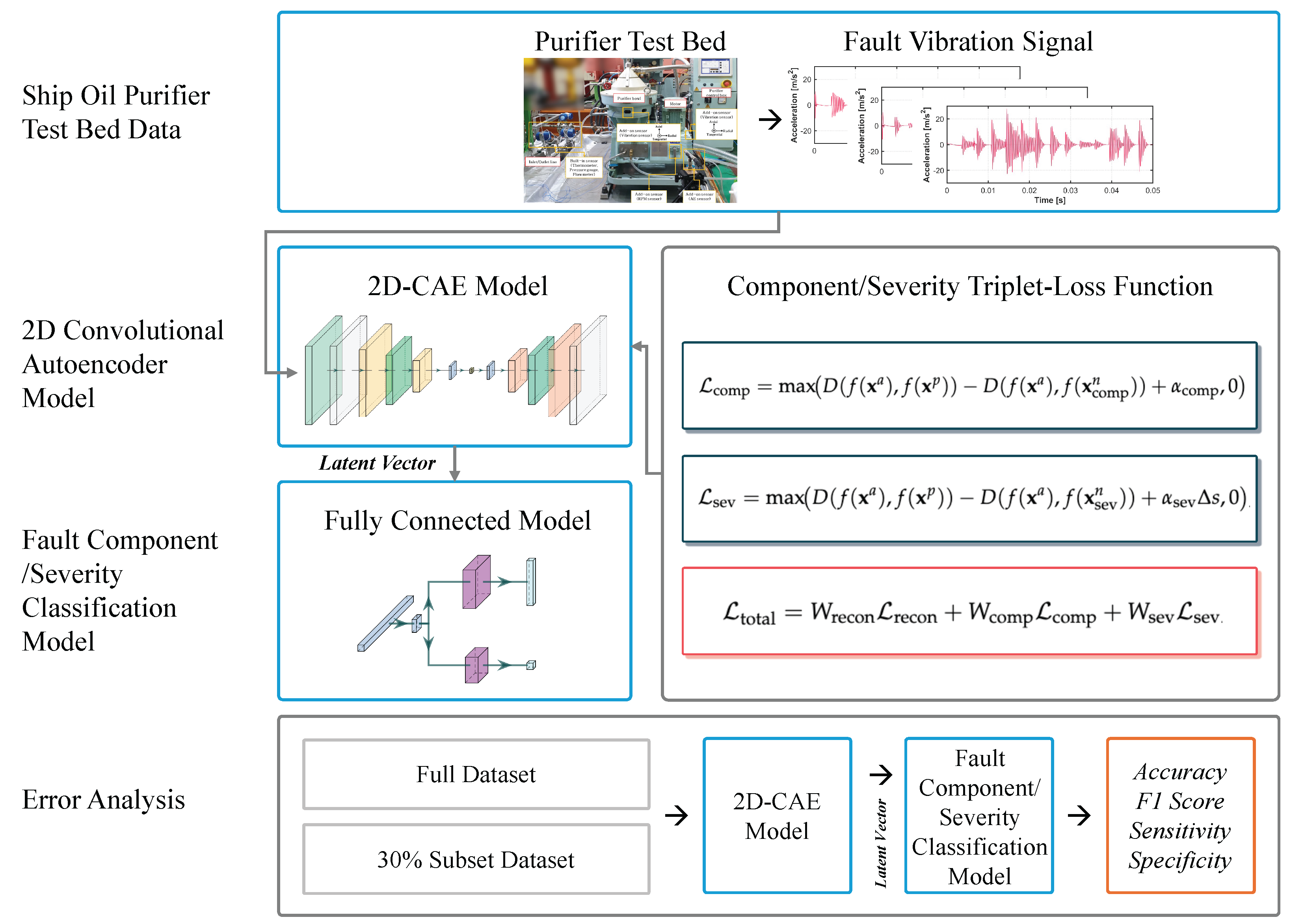Figure 5 illustrates the training loss and accuracy of the proposed AS-LSLF model. The loss curve demonstrates stable convergence of the combined objective function, with the multi-task learning approach effectively balancing the reconstruction quality and latent space structuring.

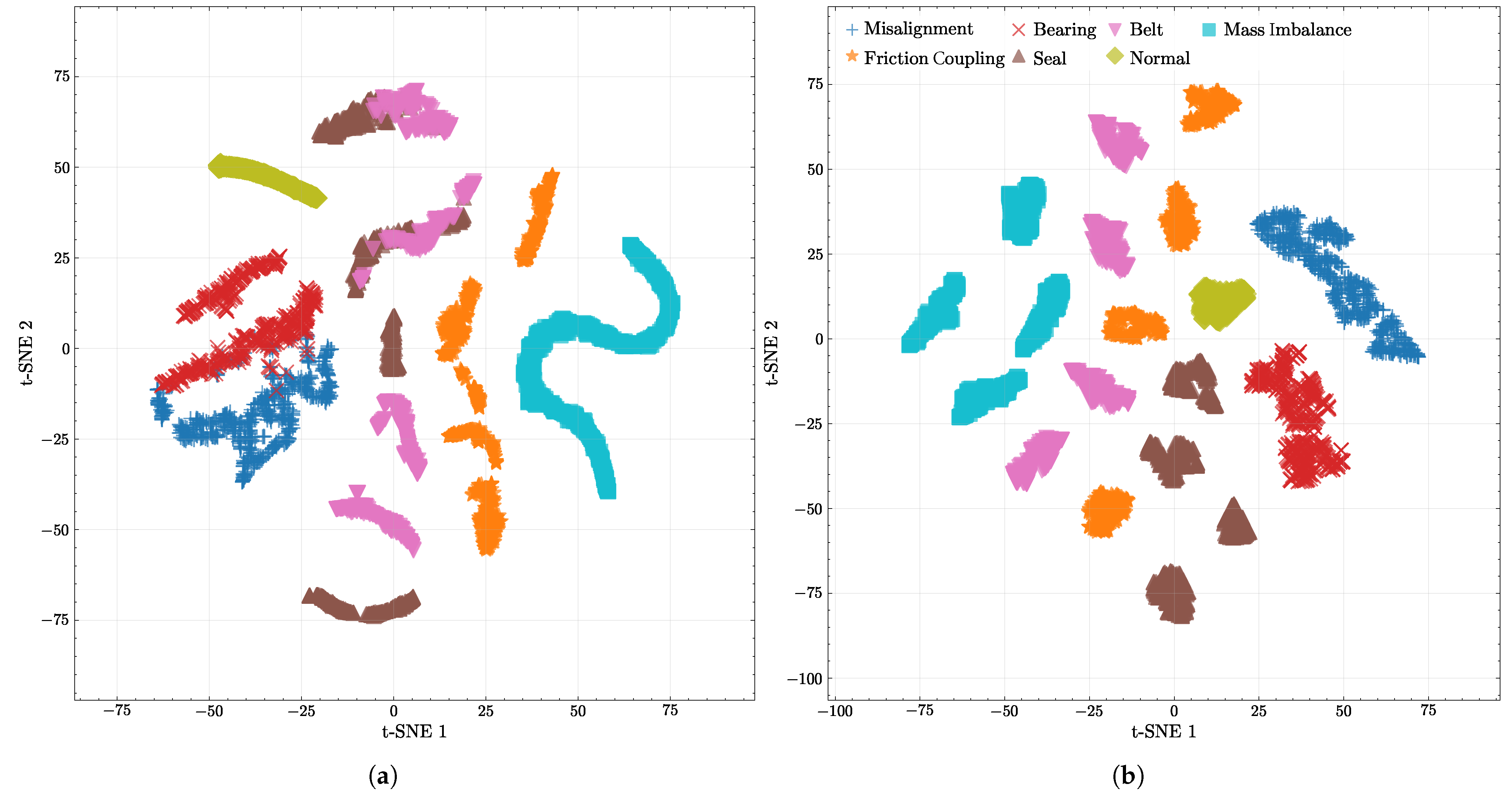
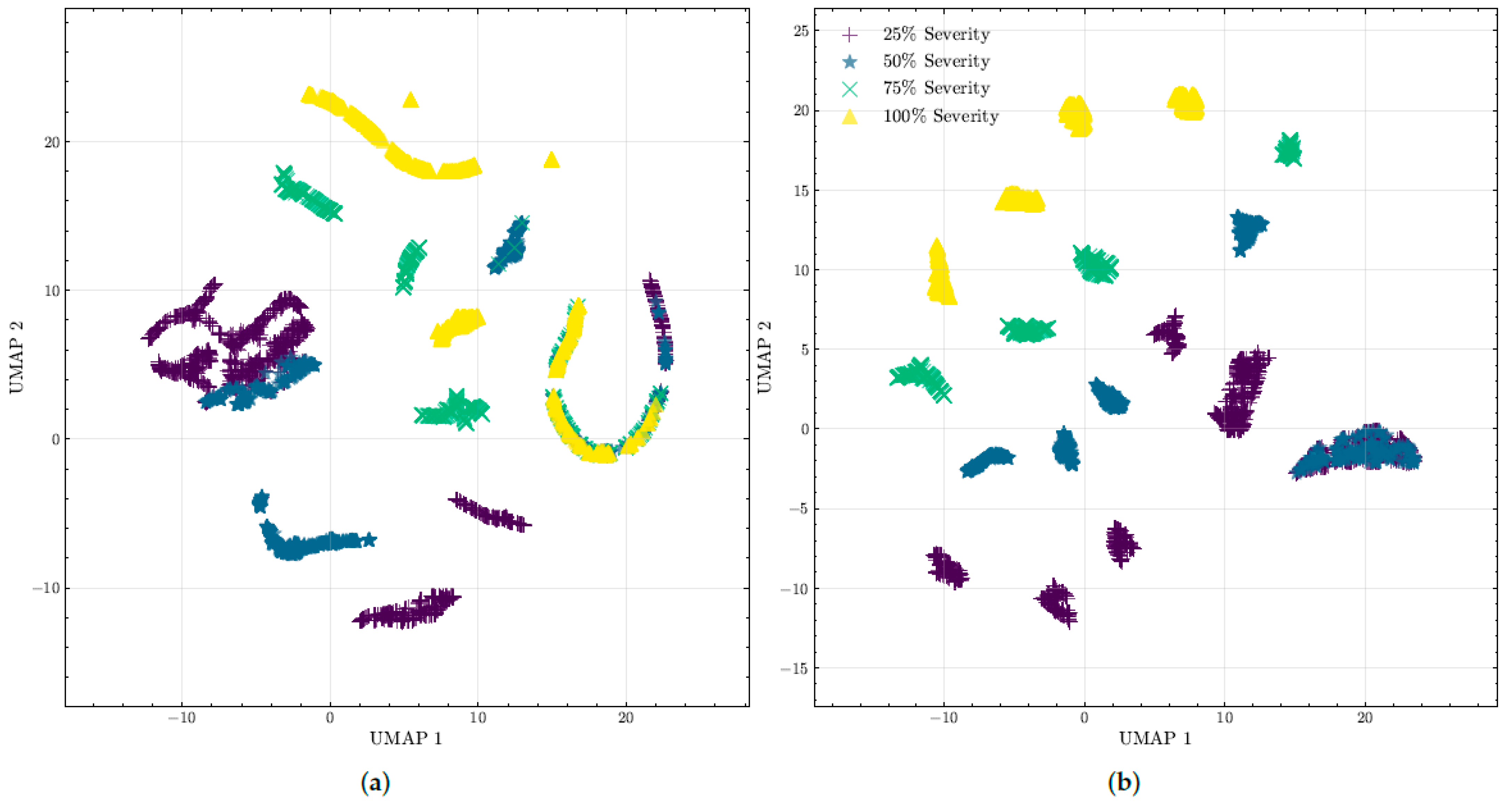
To show the capability of the proposed framework to capture the latent organization of diagnostic measurements, we visualized the latent vector from the baseline 2D-CAE and the proposed AS-LSLF encoder as two-dimensional maps. Specifically, we adopted the Uniform Manifold Approximation and Projection (UMAP) [22] and t-Distributed Stochastic Neighbor Embedding (t-SNE) [23] to project the high-dimensional embeddings into a plane for qualitative assessment. UMAP provides a topology-aware low-dimensional representation that preserves both the neighborhood structure and coarse global geometry of the original space. By contrast, t-SNE emphasizes the local neighborhood fidelity by minimizing the Kullback–Leibler divergence between pairwise similarity distributions in the original space and the embedded space, offering a complementary view of the learned latent features.

Figure 6 and Figure 7 depict separability across fault component groups, while Figure 8 and Figure 9 summarize the stratification by fault severity. In the baseline 2D-CAE embeddings, several clusters intermix, indicating weaker discrimination between classes. In contrast, the proposed AS-LSLF framework yields cleaner decision regions with markedly clearer boundaries, most prominently under UMAP, demonstrating an enhanced ability to disentangle operating conditions. The reduced overlap and wider margins achieved by the proposed model indicate more discriminative latent representations than the baseline, supporting improved downstream inference and health state characterization.

This structural superiority translates into improved quantitative performance, as demonstrated in Table 3 and Table 4, which summarize the downstream classification results from both models. Additionally, Table 5, Table 6, Table 7, Table 8, Table 9 and Table 10 provide detailed quantitative results using four key metrics: Accuracy, F1 Score, Sensitivity, and Specificity. Each metric is reported separately for the component classification and severity classification using test data for performance comparison. 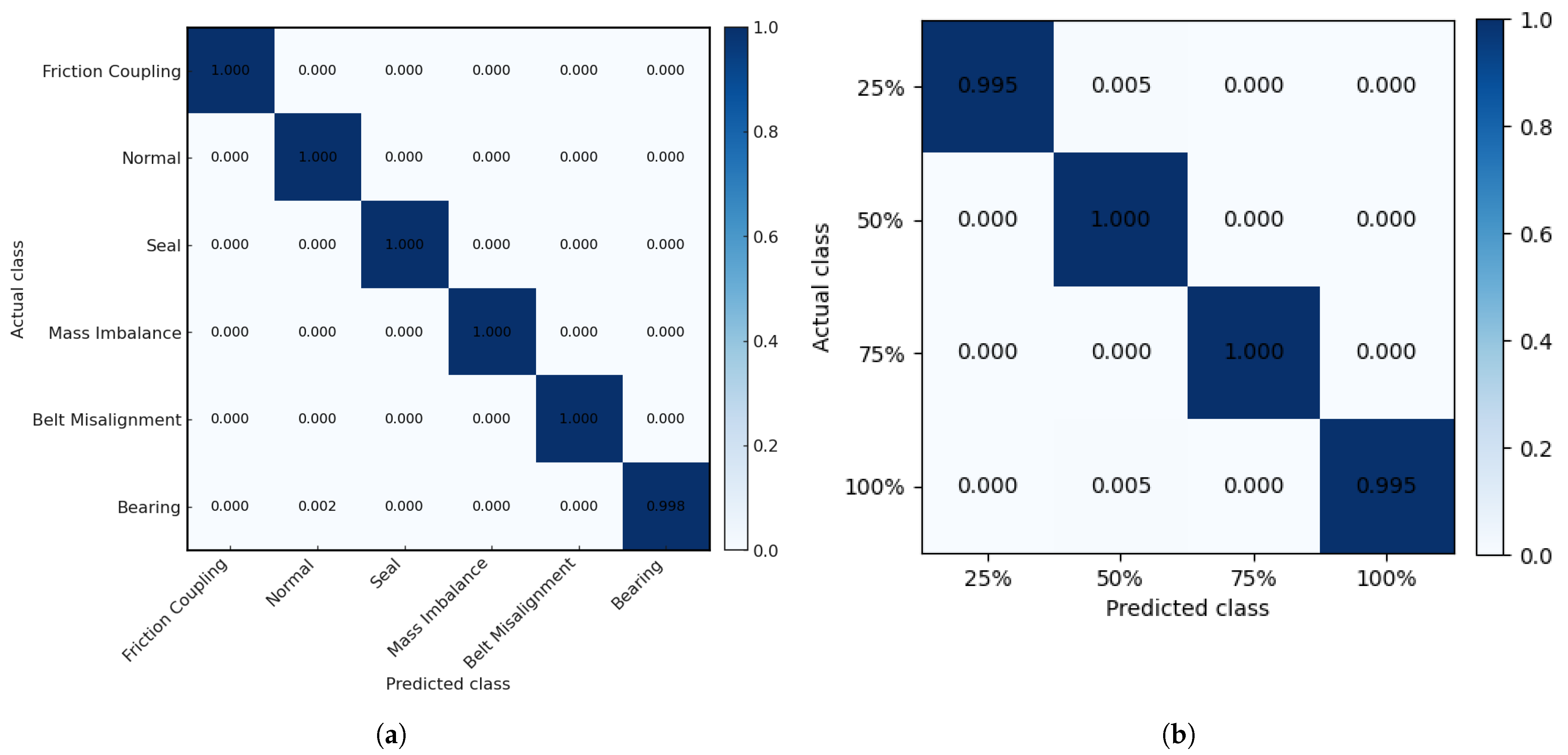Finally, Figure 10 shows the confusion matrix for component classification and fault severity classification of proposed AS-LSLF model. The performance metrics for a generic multiclass classification model are formally defined as follows:

$$\begin{array}{ccc}\hfill \mathrm{Accuracy}& =& {\displaystyle \frac{\mathrm{Number}\mathrm{of}\mathrm{Correct}\mathrm{Predictions}}{\mathrm{Total}\mathrm{Number}\mathrm{of}\mathrm{Predictions}}}\hfill \end{array}$$

(10)

$$\begin{array}{ccc}\hfill \mathrm{F}1\mathrm{Score}& =& {\displaystyle \frac{1}{N}}\sum _{i=1}^{N}2\times {\displaystyle \frac{{\mathrm{Precision}}_i\times {\mathrm{Recall}}_i}{{\mathrm{Precision}}_i+{\mathrm{Recall}}_i}}\hfill \end{array}$$

(11)

$$\begin{array}{ccc}\hfill \mathrm{Sensitivity}& =& {\displaystyle \frac{1}{N}}\sum _{i=1}^N{\displaystyle \frac{T{P}_i}{T{P}_i+F{N}_i}}\hfill \end{array}$$

(12)

$$\begin{array}{ccc}\hfill \mathrm{Specificity}& =& {\displaystyle \frac{1}{N}}\sum _{i=1}^N{\displaystyle \frac{T{N}_i}{T{N}_i+F{P}_i}},\hfill \end{array}$$

(13)

where TP (True Positive) denotes correctly predicted instances of each class, TN (True Negative) indicates correctly predicted instances not belonging to each class, FN (False Negative) indicates instances incorrectly predicted as belonging to other classes, FP (False Positive) represents instances incorrectly predicted as the given class, and N denotes the total number of classes.

Table 3. Component classification performance comparison for the ablation study.

Model	Accuracy (%)	F1 (%)	Sensitivity (%)	Specificity (%)
AS-LSLF (Proposed)	99.98	99.97	99.96	99.99
2D-CAE	99.89	99.82	99.81	99.97

Table 3. Component classification performance comparison for the ablation study.

Model	Accuracy (%)	F1 (%)	Sensitivity (%)	Specificity (%)
AS-LSLF (Proposed)	99.98	99.97	99.96	99.99
2D-CAE	99.89	99.82	99.81	99.97

Figure 6. UMAP-based projections of the learned latent manifolds from the baseline and proposed models. (a) Baseline 2D-CAE. (b) Proposed AS-LSLF.

Figure 6. UMAP-based projections of the learned latent manifolds from the baseline and proposed models. (a) Baseline 2D-CAE. (b) Proposed AS-LSLF.

Figure 7. t-SNE projections of the learned latent manifolds from the baseline and proposed models. (a) Baseline 2D-CAE. (b) Proposed AS-LSLF.

Figure 7. t-SNE projections of the learned latent manifolds from the baseline and proposed models. (a) Baseline 2D-CAE. (b) Proposed AS-LSLF.

Figure 8. UMAP visualization of the learned latent space for fault severity. (a) Baseline 2D-CAE. (b) Proposed AS-LSLF.

Figure 8. UMAP visualization of the learned latent space for fault severity. (a) Baseline 2D-CAE. (b) Proposed AS-LSLF.

Figure 9. t-SNE visualization of the learned latent space for fault severity. (a) Baseline 2D-CAE. (b) Proposed AS-LSLF.

Figure 9. t-SNE visualization of the learned latent space for fault severity. (a) Baseline 2D-CAE. (b) Proposed AS-LSLF.

Figure 10. Confusion matrix of proposed AS-LSLF model. (a) Component classification. (b) Fault severity classification.

Figure 10. Confusion matrix of proposed AS-LSLF model. (a) Component classification. (b) Fault severity classification.

Table 4. Fault severity classification performance comparison for the ablation study.

Model	Accuracy (%)	F1 (%)	Sensitivity (%)	Specificity (%)
AS-LSLF (Proposed)	99.88	99.87	99.75	99.89
2D-CAE	99.14	98.95	98.90	99.35

Table 4. Fault severity classification performance comparison for the ablation study.

Model	Accuracy (%)	F1 (%)	Sensitivity (%)	Specificity (%)
AS-LSLF (Proposed)	99.88	99.87	99.75	99.89
2D-CAE	99.14	98.95	98.90	99.35

To further assess the robustness and generalizability of our proposed model and the ablation model, we performed a five-fold cross-validation. The dataset was partitioned into five subsets of equal size. In each fold, one subset was used for testing, while the remaining four were used for training. This process was repeated five times, ensuring that each subset was used as the test set exactly once. The results, presented as the mean and standard deviation of the performance metrics across the five folds, are shown in Table 5 and Table 6. The consistently high performance across all folds with low standard deviations demonstrates the stability and reliability of our proposed approach.

Table 5. Five-fold cross-validation results for component classification.

Model	Accuracy (%)	F1 (%)	Sensitivity (%)	Specificity (%)
AS-LSLF (Proposed)	99.18 ± 0.013	99.17 ± 0.015	99.16 ± 0.014	99.19 ± 0.014
2D-CAE	98.99 ± 0.014	98.92 ± 0.015	98.91 ± 0.013	99.07 ± 0.014

Table 5. Five-fold cross-validation results for component classification.

Model	Accuracy (%)	F1 (%)	Sensitivity (%)	Specificity (%)
AS-LSLF (Proposed)	99.18 ± 0.013	99.17 ± 0.015	99.16 ± 0.014	99.19 ± 0.014
2D-CAE	98.99 ± 0.014	98.92 ± 0.015	98.91 ± 0.013	99.07 ± 0.014

Table 6. Five-fold cross-validation results for fault severity classification.

Model	Accuracy (%)	F1 (%)	Sensitivity (%)	Specificity (%)
AS-LSLF (Proposed)	99.08 ± 0.023	98.97 ± 0.014	98.85 ± 0.018	98.99 ± 0.013
2D-CAE	98.24 ± 0.025	98.05 ± 0.033	98.00 ± 0.019	98.45 ± 0.024

Table 6. Five-fold cross-validation results for fault severity classification.

Model	Accuracy (%)	F1 (%)	Sensitivity (%)	Specificity (%)
AS-LSLF (Proposed)	99.08 ± 0.023	98.97 ± 0.014	98.85 ± 0.018	98.99 ± 0.013
2D-CAE	98.24 ± 0.025	98.05 ± 0.033	98.00 ± 0.019	98.45 ± 0.024

3.2. Performance Comparison with Other Methods

To further establish the superiority of the proposed framework, its diagnostic performance was benchmarked against several state-of-the-art deep learning models commonly employed for time-series classification. The selected baselines include a two-dimensional CNN (2D-CNN) [19], a standard one-dimensional CNN (1D-CNN) [24], and a bidirectional long short-term memory network (BiLSTM) [25]. From a computational standpoint, the proposed AS-LSLF framework introduces additional complexity during training compared with a standard 2D-CNN, owing to the pairwise distance calculations required by the triplet-loss. Its inference time, however, remains comparable with the 2D-CNN. While more computationally intensive than the 1D-CNN due to its two-dimensional architecture, AS-LSLF is substantially more efficient than the BiLSTM model, whose sequential processing is inherently slower for long time series. To evaluate the robustness and data efficiency, which is critical for real-world maritime applications where acquiring extensive labeled fault data is often infeasible, the analysis was conducted under two data-utilization regimes: full and 30% of the available training data.

With full training data (Table 7 and Table 8), the proposed AS-LSLF framework outperforms all baselines across nearly every metric. The performance gap further widens under the reduced 30% dataset setting (Table 9 and Table 10); while the baseline performance drops sharply, AS-LSLF remains remarkably resilient thanks to the metric-learning composite loss that regularizes the latent space, while the BiLSTM model struggles due to lack of training data.

Table 7. Component classification performance comparison with full training data.

Model	Accuracy (%)	F1 (%)	Sensitivity (%)	Specificity (%)
AS-LSLF (Proposed)	99.98	99.97	99.96	99.99
2D-CAE	99.89	99.82	99.81	99.97
2D-CNN	99.88	99.88	99.87	99.96
1D-CNN	97.1	96.9	96.8	97.5
BiLSTM	96.68	96.40	96.20	97.10

Table 7. Component classification performance comparison with full training data.

Model	Accuracy (%)	F1 (%)	Sensitivity (%)	Specificity (%)
AS-LSLF (Proposed)	99.98	99.97	99.96	99.99
2D-CAE	99.89	99.82	99.81	99.97
2D-CNN	99.88	99.88	99.87	99.96
1D-CNN	97.1	96.9	96.8	97.5
BiLSTM	96.68	96.40	96.20	97.10

Table 8. Fault severity classification performance comparison with full training data.

Model	Accuracy (%)	F1 (%)	Sensitivity (%)	Specificity (%)
AS-LSLF (Proposed)	99.88	99.87	99.75	99.89
2D-CAE	99.14	98.95	98.90	99.35
2D-CNN	99.88	99.88	99.80	99.90
1D-CNN	92.43	91.98	91.50	93.80
BiLSTM	78.13	78.09	78.09	82.50

Table 8. Fault severity classification performance comparison with full training data.

Model	Accuracy (%)	F1 (%)	Sensitivity (%)	Specificity (%)
AS-LSLF (Proposed)	99.88	99.87	99.75	99.89
2D-CAE	99.14	98.95	98.90	99.35
2D-CNN	99.88	99.88	99.80	99.90
1D-CNN	92.43	91.98	91.50	93.80
BiLSTM	78.13	78.09	78.09	82.50

Table 9. Component classification performance comparison with 30% training data utilization.

Model	Accuracy (%)	F1 (%)	Sensitivity (%)	Specificity (%)
AS-LSLF (Proposed)	99.88	99.87	99.75	99.89
2D-CAE	97.71	97.30	96.80	97.90
2D-CNN	97.90	97.6	97.5	98.1
1D-CNN	94.34	93.76	92.50	94.80
BiLSTM	71.88	63.06	58.40	75.20

Table 9. Component classification performance comparison with 30% training data utilization.

Model	Accuracy (%)	F1 (%)	Sensitivity (%)	Specificity (%)
AS-LSLF (Proposed)	99.88	99.87	99.75	99.89
2D-CAE	97.71	97.30	96.80	97.90
2D-CNN	97.90	97.6	97.5	98.1
1D-CNN	94.34	93.76	92.50	94.80
BiLSTM	71.88	63.06	58.40	75.20

Table 10. Fault severity classification performance comparison with 30% training data utilization.

Model	Accuracy (%)	F1 (%)	Sensitivity (%)	Specificity (%)
AS-LSLF (Proposed)	99.87	99.80	99.80	99.90
2D-CAE	95.77	95.63	95.63	99.56
2D-CNN	94.21	93.95	93.95	99.26
1D-CNN	90.38	89.46	89.46	98.11
BiLSTM	61.92	58.62	58.62	90.44

Table 10. Fault severity classification performance comparison with 30% training data utilization.

Model	Accuracy (%)	F1 (%)	Sensitivity (%)	Specificity (%)
AS-LSLF (Proposed)	99.87	99.80	99.80	99.90
2D-CAE	95.77	95.63	95.63	99.56
2D-CNN	94.21	93.95	93.95	99.26
1D-CNN	90.38	89.46	89.46	98.11
BiLSTM	61.92	58.62	58.62	90.44

4. Conclusions

This paper introduced an adaptive structured latent space learning framework designed to address the critical need for accurate, interpretable, and data-efficient fault diagnosis in ship oil purifiers, a key enabling technology for degree-4 maritime autonomous surface ships. By integrating a two-dimensional convolutional autoencoder with a component-aware triplet-loss function, our framework moves beyond conventional classification-driven objectives. The core improvement lies in the composite loss, which simultaneously optimizes for signal reconstruction fidelity, categorical separation of faults by their physical origin, and ordinal arrangement according to fault severity. The experimental results, validated on a dedicated oil purifier test bed, demonstrate the efficacy of our approach. The ablation study visually and qualitatively confirmed that the proposed triplet-loss successfully sculpts the latent space into a highly structured and physically meaningful manifold, where the latent vector is organized by both the component and severity. Furthermore, the comprehensive comparative analysis against state-of-the-art deep learning models revealed the superior performance of our framework. It not only achieved a higher diagnostic accuracy but also exhibited exceptional robustness under data-scarce conditions, a testament to the powerful regularization effect of metric learning. The proposed framework thus provides a robust and interpretable solution for condition-based maintenance, advancing the operational reliability and safety of autonomous maritime systems. Future work will focus on three primary avenues. First, we aim to validate the framework under complex, non-stationary conditions of real-world maritime operations to verify its robustness and effectiveness. Second, we will explore the integration of the structured latent space with prognostic models to enable accurate prediction of remaining useful life (RUL), transitioning from diagnostics to prognostics. Finally, the framework will be extended to incorporate additional sensor modalities, such as thermal and acoustic data, to build a more holistic and resilient diagnostic system for the critical machinery of autonomous ships.