Machine Learning-Based Condition Monitoring with Novel Event Detection and Incremental Learning for Industrial Faults and Cyberattacks

Abstract

This study presents an integrated condition-monitoring approach for industrial processes. The proposed approach conveniently combines a computational intelligence-based mechanism to guarantee the resilience of the proposed scheme against unknown anomalies and a machine learning model with optimized parameters capable of unified detection and pinpointing of faults and cyberattacks in industrial plants. During the offline phase, process data are labeled, normalized, and used to train the machine learning model with hyperparameter tuned by using an optimization tool. In the online phase, the system performs real-time monitoring enhanced with a novelty mechanism to detect anomalous conditions not present in the training data, which are flagged for expert analysis and incorporated into the system through incremental learning. The implementation of the proposed strategy uses computational intelligence tools consisting of a multilayer perceptron neural network, local outlier factor, and differential evolution. The proposed framework was validated using the two-tank process benchmark, demonstrating superior detection accuracy of 99% and robustness compared to other machine learning algorithms. These results highlight the potential of combining fault diagnosis and cybersecurity in a unified architecture, thereby contributing to resilient and intelligent systems in the context of Industry 4.0/5.0.

1. Introduction

The fourth industrial revolution signifies a revolutionary shift in manufacturing and corporate environments, fueled by the convergence of cutting-edge innovations such as the Industrial Internet of Things (IIoT), Cloud and Edge Computing, Big Data, Artificial Intelligence (AI), and Robotics [1]. Such advancements allow industries to enhance interconnectivity, automate workflows, and digitize operations, transforming legacy facilities into intelligent and interconnected Cyber-Physical Systems (CPS) [2,3]. While this fusion brings substantial advantages such as improved efficiency, higher product quality, and better compliance with safety standards, it also presents new challenges, especially concerning process-related faults and cybersecurity risks [4].

On the other hand, Industry 5.0 emphasizes a human-centered, sustainable, and resilient approach to industrial production. This paradigm shift requires sophisticated monitoring systems capable of ensuring the reliability of collaborative environments between humans and robots. Therefore, the incorporation of a condition monitoring system for the detection and localization of faults and cyberattacks directly contributes to this vision, as it allows to improve resilience and reliability of industrial processes.

Process-related faults and cyberattacks present serious threats to industrial operations, potentially resulting in decreased productivity, higher operational expenses, and safety risks [5,6]. To address these risks, industrial facilities need sophisticated Condition Monitoring (CM) systems that can promptly recognize these types of abnormal operation conditions [7,8]. However, accomplishing this objective is challenging as result of the common noisy observations obtained from the processes, which make it difficult to correctly classify whether or not the operating conditions are correct. Moreover, cyberattacks are frequently crafted to imitate typical plant operation, making their recognition even more difficult [9].

The most of the current approaches for identifying faults and cyber threat detection generally follow two principal classifications, namely, model-based and data-driven approaches [10]. Model-based methods depend on a thorough understanding of the plant behavior; however, achieving this is no easy task, especially given the complexity of contemporary industrial infrastructures. On the other hand, data-driven techniques utilize historical data to detect patterns linked to faults and attacks, offering greater flexibility and adaptability in complex and evolving environments [11].

The progressive deterioration of critical components in industrial automation systems, particularly sensors, actuators, and pumping systems, directly correlates with the occurrence of new faults. Furthermore, the fast evolution of industrial network environment as well as advanced tools and techniques used by hackers facilitate the launching of new and sophisticated attacks. For this reason, a key feature of CM systems should be the inclusion of a scheme to detect unrecognized operation conditions along with a mechanism for incremental learning which allows for resilience and improved performance [12,13].

Recent developments in AI, especially in Machine Learning (ML), highlight its strong potential to overcome CM system difficulties through robust data analysis and increased classification accuracy, despite uncertainties and mixed Fault/Attack (F/A) patterns [14,15]. However, the effectiveness of ML methods is highly reliant on proper parameter selection, which continues to be a significant challenge in their practical implementation [16].

On the other hand, a CM scheme should combine fault and attack detection with pinpointing capabilities, tackling these challenges through an integrated system that maintains operational reliability and security and fosters the synergy between the Operations Technology and Information Technology teams at industrial plants [17].

Therefore, this paper addresses the following research question:

• How can a machine learning-based condition monitoring system be designed to ensure resilience against unknown anomalies while simultaneously enabling the unified detection and pinpointing of faults and cyberattacks in industrial plants?

The main contribution of this paper is the development of a condition monitoring strategy in two stages with two principal capabilities:

• A computational intelligence-based mechanism to identify unknown events, which allows for incremental learning and ensures resilience against new risks.
• A machine learning model with optimized parameters, providing a classification tool with the ability to detect and pinpoint both faults and cyberattacks in a unified manner.

The rest of this paper is structured as follows: Section 2 presents an analysis of recent approaches proposed for the detection and localization of faults and cyberattacks; Section 3 presents the main features of the computational tools utilized in the research and the proposed condition monitoring strategy; Section 4 presents the case studies used to test the proposed scheme along with the developed experiments and an analysis of the outcomes; finally, the paper ends with our conclusions.

2. Related Works

The Introduction section explains several condition monitoring strategies proposed for industrial processes in recent years. A common characteristic of most of these approaches is that they address fault diagnosis and industrial cyberattacks separately.

The drive for greater resource efficiency and productivity in industrial processes has spurred interest in approaches that integrate both Operational Technology (OT) and Information Technology (IT) [18,19]. Motivated by this convergence, the recent scientific literature has begun to feature integrated condition monitoring schemes designed to address this research challenge by jointly detecting and localizing faults and cyberattacks.

A novel method for cyberattack identification leveraging process monitoring technology was introduced by [20]. Upon fault detection, the technique employs delayed mutual information for root cause analysis. If a state variable is identified as the root cause, the fault is attributed to a cyberattack, requiring immediate operator attention. Otherwise, the event is classified as a process fault, initiating an integrated routine response.

While [21] developed a method for simultaneous fault and cyberattack detection via two filters and an unknown input observer, [22] presented a distinct approach. Their cyber–physical event reasoning system delivers real-time diagnostics for both known and novel incidents without dependence on past data. It uses a two-stage process to infer key event aspects such as occurrence, location, root cause, and physical consequences.

To enhance overall safety and security, [23] introduced a system utilizing a Bayesian Network (BN) to account for the probabilistic nature of diverse risks. Separately, [24] proposed an integrated system for diagnosing faults and cyberattacks in industrial control systems. Their methodology was based on two core components: (1) partial models of the process in its normal state, and (2) a fault isolation system built on expert knowledge, which maps the relationships between faults and diagnostic signals to detect and isolate anomalies.

Most current methodologies are dependent on mathematical models, necessitating comprehensive understanding of process parameters, characteristics, and operational regimes. This poses a significant challenge due to the complex nonlinearities, high noise levels, and frequent disturbances present in contemporary industrial environments. These constraints underscore the pressing need for the development of novel approaches that circumvent these inherent limitations.

3. Tools and Methodology

This work proposes a two-stage strategy for a condition monitoring system. This strategy conveniently combines a computational intelligence-based mechanism to guarantee the resilience of the proposed scheme against unknown anomalies using incremental learning, and a Machine Learning model with optimized parameters for the unified detection and pinpointing of faults and cyberattacks in industrial plants.

This section first provides a summary of the computational tools employed to implement the proposed condition monitoring strategy. Next, a detailed analysis of the proposed condition monitoring scheme is presented.

3.1. General Characteristics of Computational Tools

3.1.1. Multilayer Perceptron Neural Network

Currently, many and sophisticated architectures and artificial neural networks have been presented in the scientific literature. The performance achieved by each kind has a very close relationship with the application type. In this paper, the well known Multilayer Perceptron (MLP) architecture is used. MLP is a well-known tool with outstanding results in pattern recognition applications [25].

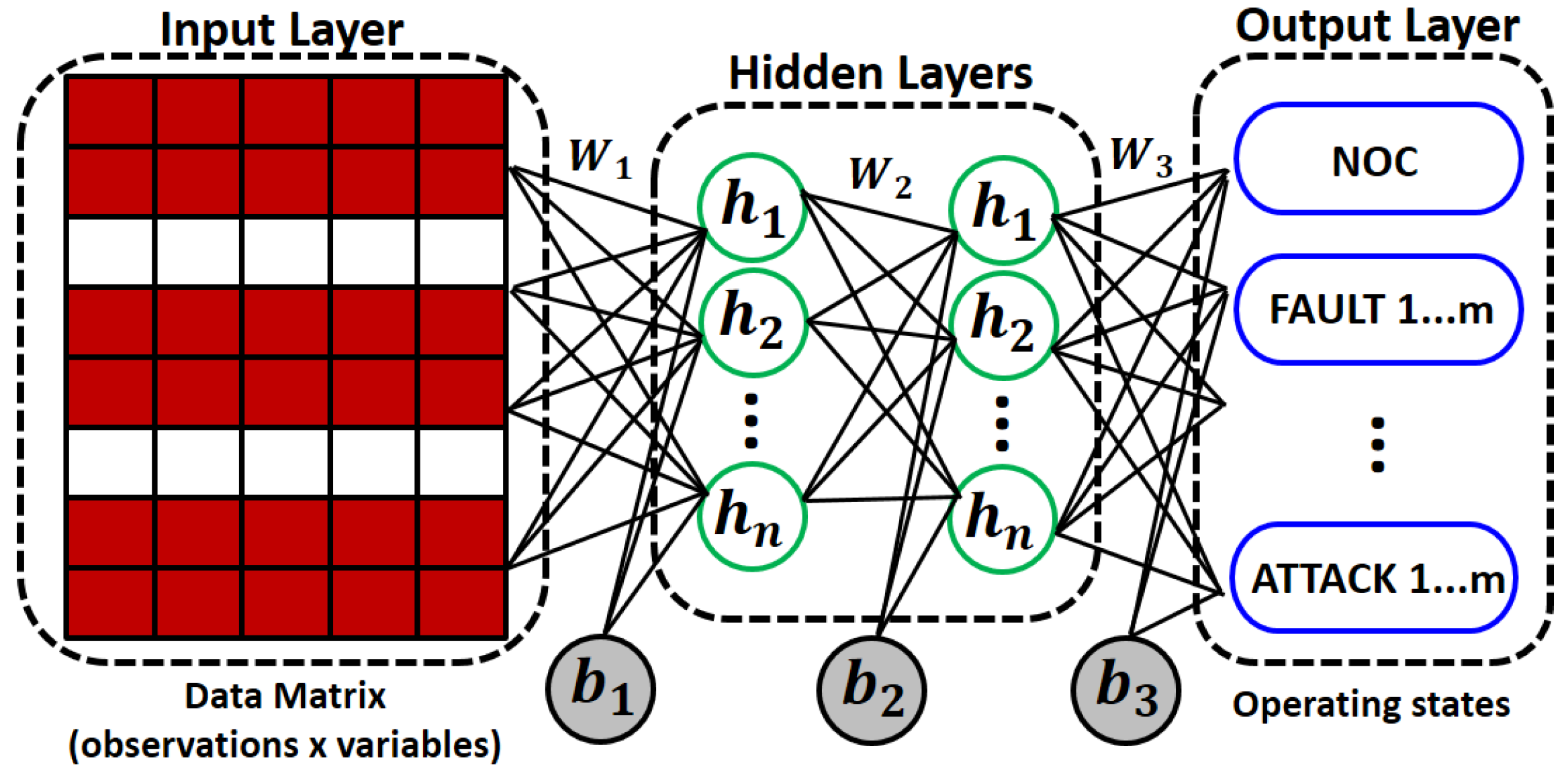
As illustrated in Figure 1, the MLP structure is organized hierarchically as follows: (1) an input layer receiving the raw data matrix (observations x variables); (2) one or more hidden layers for feature transformation; and (3) an output layer producing predictions. Our work addresses multiclass classification (Normal Operating Condition (NOC), Faults, and Attacks). These layers form a densely connected network in which each neuron communicates with all neurons in the next layer. The system operates bidirectionally: Forward Propagation (FP) computes outputs from inputs, while Backward Propagation (BP) adjusts parameters based on errors.

3.1.2. Local Outlier Factor (LOF)

The Local Outlier Factor (LOF) is a density-based unsupervised anomaly detection algorithm that identifies outliers by measuring how isolated they are from their local neighbors [26]. Its key concept is that outliers have significantly lower density compared to their neighbors. The LOF determines a sample’s local density from the distances to its neighbors. To determine it, different parameters are used:

Neighborhood of distance h ($N_h\left(x_i\right)$): Refers to the set of points with a distance to $x_i$ that is less than or equal to that of the h-th nearest neighbor of $x_i$. This set may contain h or more points depending on distance ties.

Reachability Distance $R{D}_h(x_i,x_j)$: Defined as the maximum between the h-distance of $x_j$ and the actual distance from $x_i$ to $x_j$. This distance is formally provided by Equation (1).

$$R{D}_h(x_i,x_j)=max(distanc{e}_h\left(x_j\right),distance(x_i,x_j))$$

(1)

Local Reachability Density $LR{D}_h\left(x_i\right)$: Defined as the inverse of the mean reachability distance from $x_i$ to its neighbors. This quantity is formally expressed in Equation (2).

$$LR{D}_h\left(x_i\right)={\displaystyle \frac{1}{\frac{{\sum }_{x_j\in N_h\left(x_i\right)}R{D}_h(x_i,x_j)}{|N_h\left(x_i\right)|}}}$$

(2)

From these parameters, the outlier factor can be calculated by applying Equation (3). The procedure of the LOF algorithm is provided in Figure 2.

$$LO{F}_h\left(x_i\right)={\displaystyle \frac{{\sum }_{x_j\in N_h\left(x_i\right)}LR{D}_h\left(x_j\right)}{|N_h\left(x_i\right)|}}\ast {\displaystyle \frac{1}{LR{D}_h\left(x_i\right)}}$$

(3)

3.1.3. Differential Evolution

Operating on a population-based approach, Differential Evolution (DE) is an algorithm that draws inspiration from biological processes. It aims to evolve a new generation of solutions by strategically changing individuals from the actual population. This is achieved through a sequence of mutation, crossover, and selection operations. A detailed explanation of this algorithm can be found in [27]. The DE algorithm is shown in Algorithm 1, and the stopping criteria used are as follows: (1) maximum number of iterations ($Itr\_max$) and (2) value of the objective function.

Algorithm 1 Differential Evolution

1: Input: population, escalation factor, crossover factor, $Itr\_max$.   2: Output: best individual in the population ($F\left(\widehat{\theta }\right)$ = $Ne$)   3: Create an initial population.   4: Choose the optimal solution.   5: for $l=1$ to $l=Itr\_max$ do   6:      Perform Mutation   7:      Perform Crossover   8:      Perform Selection   9:      Update optimal solution 10:      Check the Stopping criterion 11: end for

3.2. Proposed CM Methodology

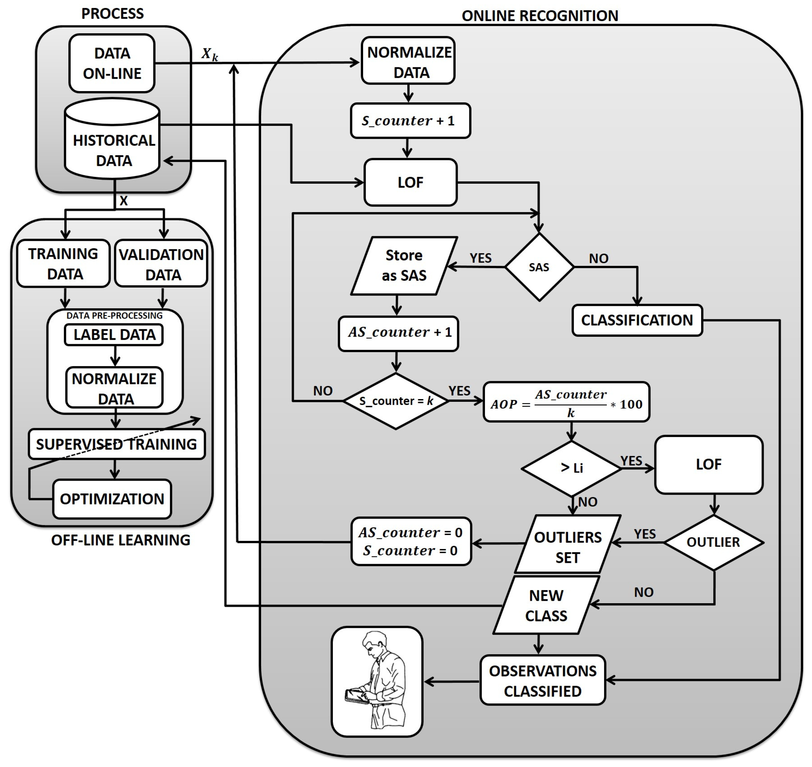
As depicted in Figure 3, the CM approach enables the detection and pinpointing of faults and cyberattacks. This adaptable strategy is suitable for diverse process industries.

3.2.1. Offline: Training Stage

The training phase is a main step in the CM strategy. To generate an artificial neural network (in this paper, an MLP) capable of detecting and identifying faults and cyberattacks in an industrial plant, the following steps are essential: data preprocessing, architecture design, training, parameter optimization, and validation.

The preprocessing phase commences with data labeling for each class. Subsequently, the dataset must be normalized; this crucial step prevents variables with higher magnitudes from overshadowing those with smaller ones, guaranteeing that the pertinent data are saved for training. The dataset is then divided, with 80% allocated to the training set (70%/10% − training/validation) and the remaining 20% reserved for the test set.

The validation data assess how well the model performs on the training set as its parameters are adjusted. This strategic data splitting is crucial for mitigating issues such as overfitting and underfitting. Following network configuration, the training process commences. Upon completion, the trained network is then deployed on the test dataset to forecast the current process state and determine the accuracy for each class.

Next, a crucial optimization step is developed to fine-tune the neural network parameters. In this step, an optimization algorithm estimates the number of neurons ($Nn$) in the different hidden layers ($ly$) by optimizing an objective function. This automated approach for determining $Nn$ leads to a better performing network configuration, ultimately enhancing classification accuracy in the real time phase.

As indicated in Equation (4), the Mean Square Error (MSE) serves as the objective function.

$$MSE={\displaystyle \frac{1}{N}}\sum _{i=1}^N{\left(A_i-{\widehat{A}}_i\right)}^2$$

(4)

Here, the Mean Squared Error (MSE) reflects the classification error, with N denoting the sample size, $A_i$ representing the best accuracy (where Acc = 1), and ${\widehat{A}}_i$ being the accuracy predicted by the ANN.

Thus, the optimization task is formulated as shown below.

$$\begin{array}{ccc}\hfill min\left\{MSE\right\}& =& {\displaystyle \frac{1}{N}}\sum _{i=1}^N{\left(A_i-{\widehat{A}}_i\right)}^2\hfill \\ \hfill s.t.\\ \hfill N{n}_{min}^1& \le & N{n}^1\le N{n}_{max}^1\hfill \\ \hfill N{n}_{min}^2& \le & N{n}^2\le N{n}_{max}^2\hfill \\ \hfill ⋮\\ \hfill N{n}_{min}^{ly}& \le & N{n}^{ly}\le N{n}_{max}^{ly}\hfill \end{array}$$

Across numerous scientific disciplines, a wide array of algorithms founded on distinct operational principles and theoretical foundations have been successfully employed to tackle optimization problems, with notable results. Several of them can be used to develop the above optimization task. Biologically-inspired algorithms fall within this array [28,29], achieving strong convergence toward the global optimum in the majority of cases along with a balanced computational effort.

The Differential Evolution (DE) algorithm is used in this study to optimize the values of parameters $N{n}^1$, $N{n}^2$, …$N{n}^{ly}$. Its selection is based on its ease of implementation and strong performance [30]. The stopping criteria were the maximum number of iterations ($Itr\_max$) and value of the objective function.

3.2.2. Online: Recognition Stage

In this phase (Figure 3), the monitoring system analyzes each observation in real time. It classifies observations as Normal or Abnormal Operating Condition (NOC, AOC), encompassing known faults and attacks. Unrecognized events are flagged as Anomalous Samples (SAS).

This stage allows the proposed scheme to detect new events. Experts establish a temporal window of k samples and a criterion $Li$. The parameter k is selected based on process characteristics and reflects the number of consecutive samples that experts consider sufficient to assess possible novel occurrences. $Li$ represents the percentage of samples classified as anomalous within the set of k samples that require analysis to confirm a possible novel pattern.

This paper introduces a new strategy for real time detection of novel patterns (Algorithm 2). In this stage, the LOF algorithm evaluates each new sample to determine whether it belongs to a known operational state [31,32,33]. The LOF classifier achieves this by constructing a decision limit around the training data. In the online stage, observations falling outside this limit are identified as abnormal (SAS). When a sample matches a recognized operational state, the machine learning algorithm assigns it to the corresponding category. Unidentified samples flagged as anomalous are stored in memory while the AS counter increases. The procedure iterates until the specified window of k observations has been fully processed.

Following classification of the k observations, the percentage classified as anomalous observations ($AOP=AS\ast 100/k$) is calculated. In the case where the $AOP$ does not exceed $Li$, the observations cannot be considered as a new class, and the AS counter is initialized for a new count. When $AOP$ is greater or equal than $Li$, the set of abnormal samples ($SAS$) undergoes evaluation to determine whether they signify a novel Fault/Attack (F/A) pattern or are outliers. The possible situation in which a new pattern indicates a changed operational state is not considered here.

To assess the set of SAS, the LOF algorithm is used. It works under the principle that a set of outliers do not achieve a density value that ensures the existence of a new pattern. Conversely, when a new event emerges, the density of the sample set is high, indicating the existence of a new class. This algorithm is used to determine whether or not the set of k abnormal samples represents a new pattern.

When the set of SAS manifests as a novel class, it is necessary for the expert to discern whether it aligns with an F/A pattern. After the identification and characterization of a new class is accomplished, if it is indeed proven to be a novel form of F/A, it is archived in the historical dataset of the process and utilized in the training stage. Afterwards, the classification algorithm requires retraining and systematic iteration of online monitoring is performed with a novel F/A identification step. This online process facilitates the automated detection of new faults and cyberattacks, which ensures the resilience and robustness of the proposed system through an incremental learning process.

Algorithm 2 Online: Classification

1: Input: data $x_k$, h-neighbors.   2: Output: Current State.   3: Choose k   4: Choose $Li$   5: Initialization $Scounter=0$   6: Initialization $AScounter=0$   7: for $j=1$ to $j=k$ do   8:     $Scounter=Scounter+1$   9:     Predict class, based on the trained LOF classifier. 10:     if k ∉ Anomalous Sample (SAS) then 11:         Apply the ML-based classifier. 12:         Identify the known class to which the sample k belongs. 13:     else 14:         Store sample k as $SAS$. 15:         $AScounter=AScounter+1$ 16:     end if 17: end for 18: Calculate $AOP$ = ${\displaystyle \frac{\left(AScounter\right)\ast 100}{k}}$ 19: if $AOP$ > $Li$ then 20:     Apply LOF algorithm for $SAS$ considering two class (New Event, Outlier). 21:     if $SAS$ ∉ $C_{outlier}$ then 22:         Create a new class. 23:         Identify the new class: Fault or Attack. 24:         Save to the historical database for use in later training. 25:     else 26:         Delete Outliers Set 27:         $AScounter=0$ 28:         $Scounter=0$ 29:     end if 30: else 31:     Delete Outliers Set 32:     $AScounter=0$ 33:     $Scounter=0$ 34: end if

4. Application of the Proposed Approach

This section present two examples demonstrating the application of the proposed CM scheme.

4.1. An Illustrative Example Using the Diamond Dataset

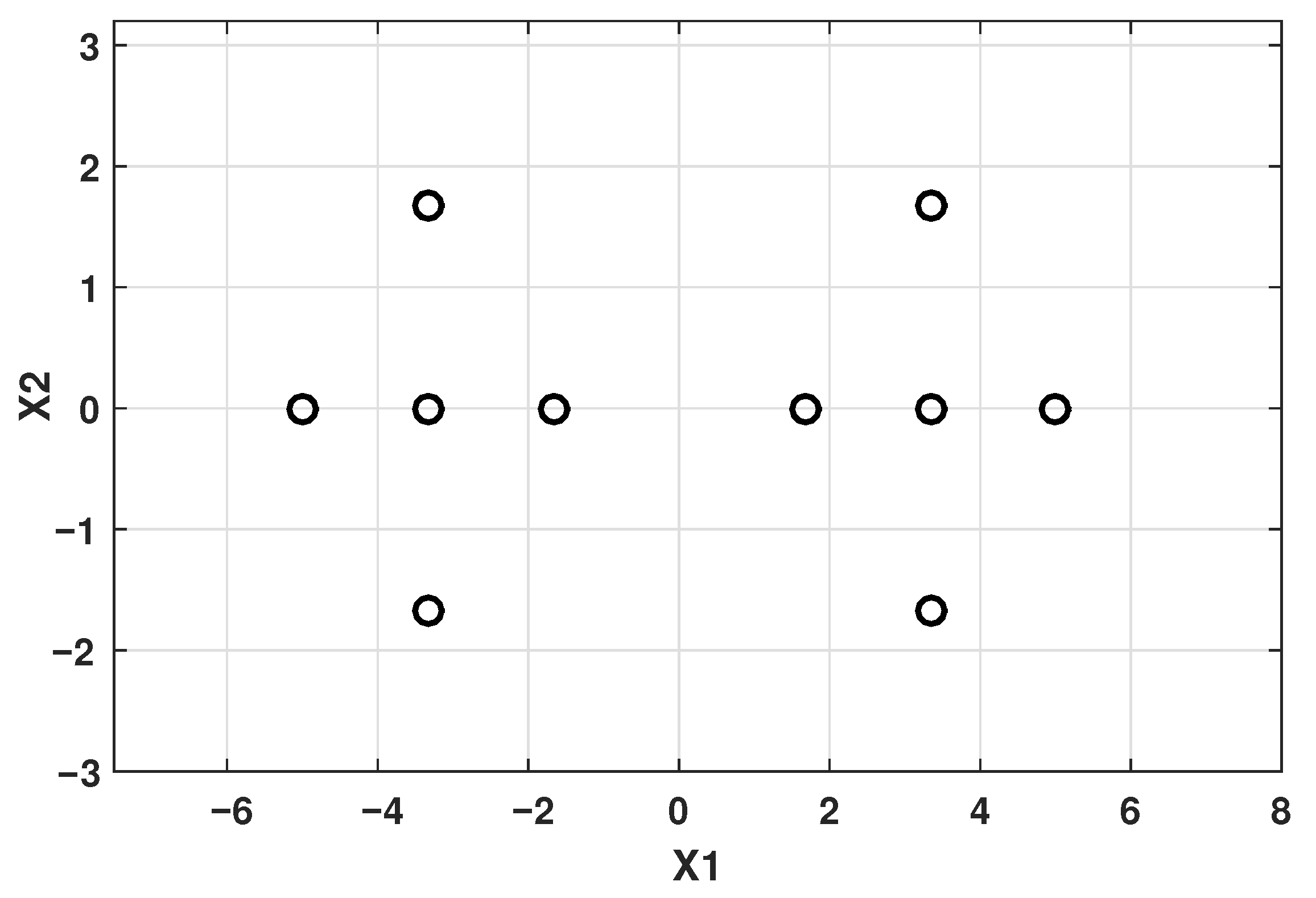
This dataset (See Figure 4) is utilized to demonstrate three examples of the proposed monitoring system featuring automatic learning capabilities. The dataset contains two classes, each with five observations, and each class is characterized by two variables, $x_1$ and $x_2$ [34].

4.1.1. Analysis and Discussion of Results

Offline: Training Stage

This example uses very little data, with the main objective being to visualize the performance of the online stage for detecting new classes. The MLP algorithm was used during the training process. To construct the neural network model, the parameters were configured with an output layer consisting of two neurons (representing the two classes) and a softmax activation function.

Table 1. Parameters of the MLP model optimized using the DE algorithm for the diamond dataset).

Parameter	Value
$Nn$ layer	1
$Nn$ Layer 1	$N{n}^1$
Cost function	Cross Entropy
Optimization function	Adam

shows the hyperparameters used in the MLP model.

To determinate the parameter $Nn$, the DE computational tool was used. The population size P, crossover constant $C_O$, and scaling factor $F_E$ were used as the control parameters. The parameters were set to the following values: $C_O=0.5$, $F_E=0.1$, $P=10$, $Itr\_max$ = 100, and $MSE$ ≤ 0.0001. The search space was $1\le N{n}^l\le 10$.

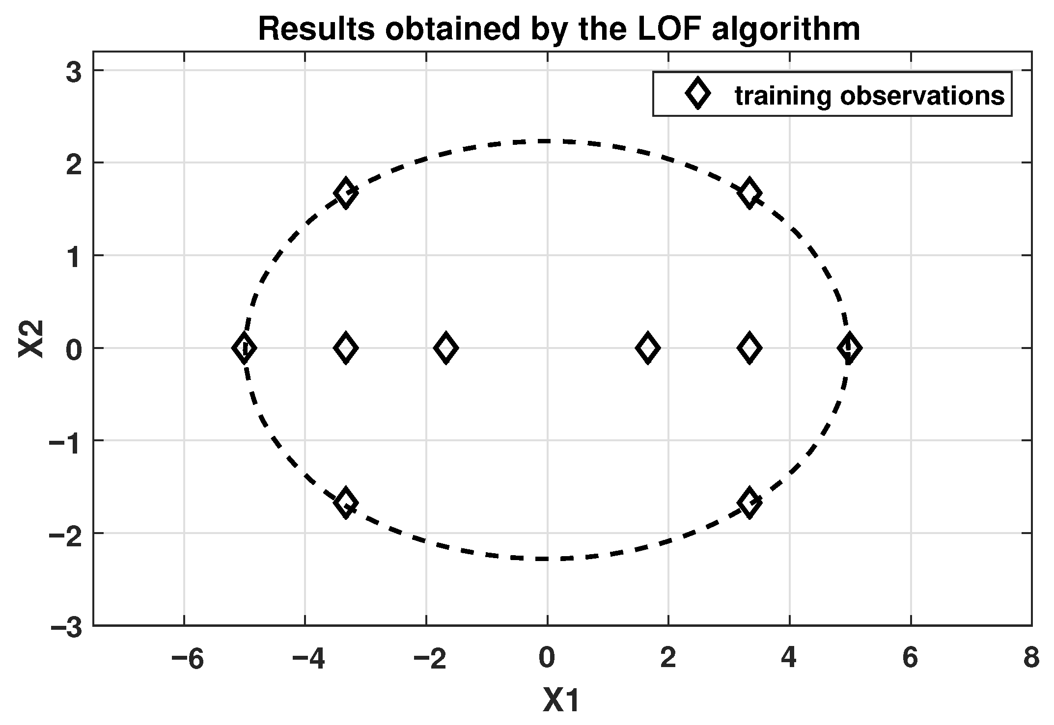
The performance of the objective function (MSE) is illustrated in Figure 5, where it is evident that the DE algorithm achieves rapid convergence. The best parameter was $N{n}^1$ = 2, obtained from iteration 4. The training error achieved by the MLP network with DE-estimated parameters is displayed in Figure 6, while Figure 7 presents the outcome of the LOF algorithm in the training phase using h = 2. Experiments were conducted to select the h-neighbors parameter in LOF, varying the number of neighbors until the best performance was determined.

Online: Recognition Stage

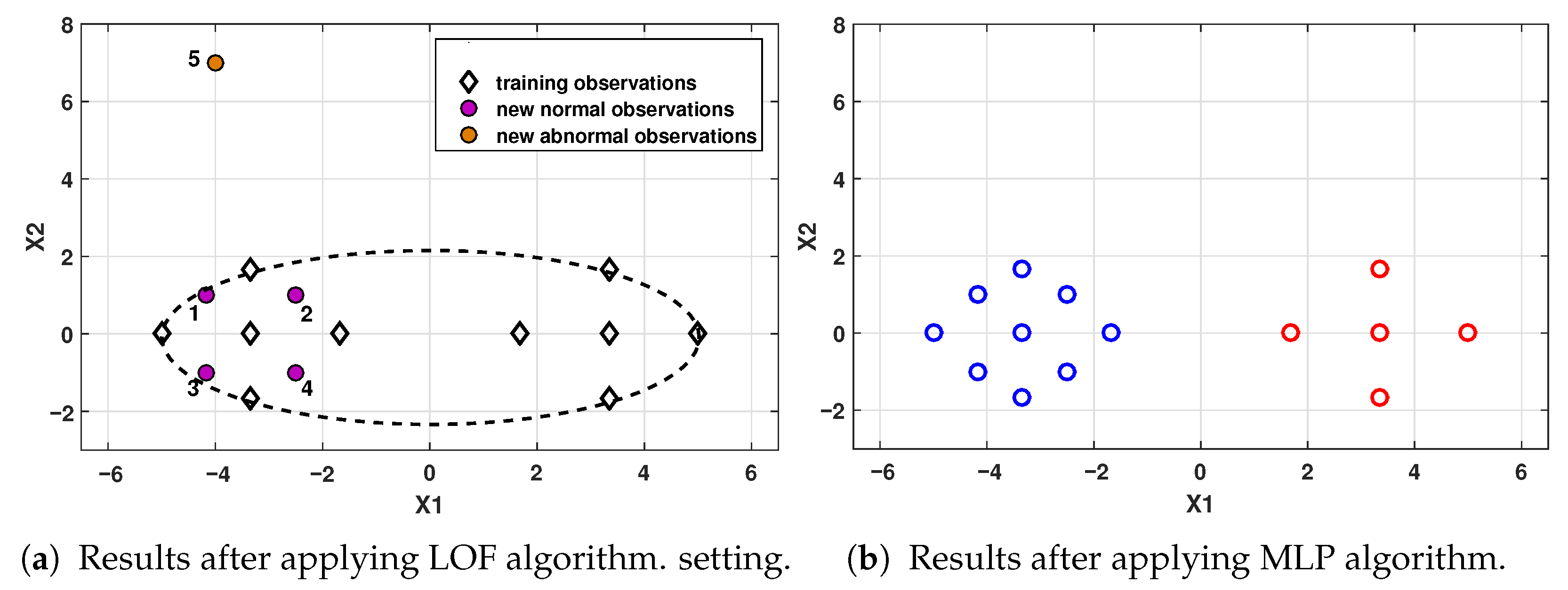
Three experiments were developed to validate the online recognition phase introduced in this study. In all examples, five observations were used to simulate the sequential acquisition of data in an online setting. The numbering associated with each observation refers to the sequence in which they arrived. For the three examples, values of $k=5$ and $Li=50\%$ were used.

• Experiment 1: Five samples were utilized, with four belonging to Class 1 and a single sample being an outlier. The goal was to assess the system’s ability to classify the samples accurately and detect a sample that represents an outlier as being SAS.
• Experiment 2: Two samples from Class 2 and three outliers that do not constitute a class were used. The aim was to analyze the system’s accuracy in classification and its ability to detect multiple outliers, such as SAS points, which do not form a new class due to their low density.
• Experiment 3: Five samples belonging to an unknown class were utilized. The aim was to analyze the appropriate classification of these samples as SAS and the capacity to detect which of these values conformed to a new pattern.

4.1.2. Result for Experiment 1

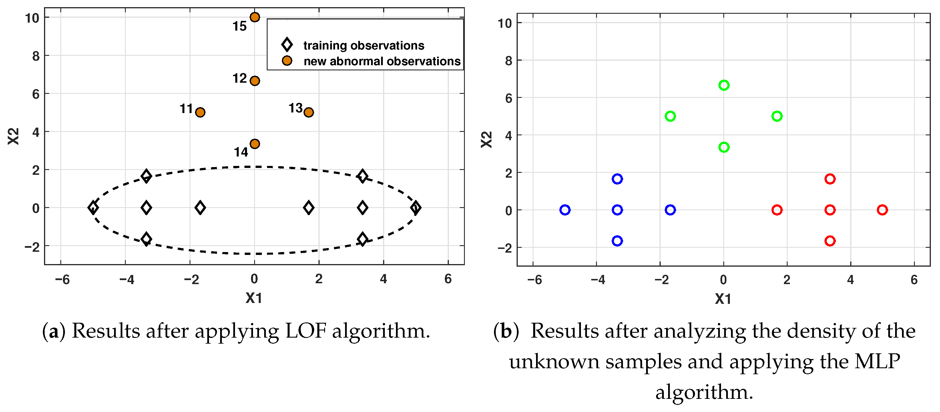
As seen in the Figure 8a, four samples were classified as known classes and the other (sample 5) as an unknown class. In this case $k=5$, AS = 1 and AOP = 20% < $Li$. Then, the observation classified as SAS was identified as an outlier. The result of the final classification of the known observations is shown in Figure 8b (Class 1:in blue and Class 2: in red).

4.1.3. Result for Experiment 2

Two samples were classified as known classes and three (samples 8, 9 and 10) were classified as unknown, as shown in Figure 9a. For this example, $k=5$, AS = 3, and AOP = 60% > $Li$. Analysis of the three samples classified as SAS was then performed. Following the density analysis, the LOF algorithm concluded that a new class was not formed. The final outcome of the online analysis is displayed in Figure 9b.

4.1.4. Result for Experiment 3

In this case, five samples were identified as unknown classes (See Figure 10a). For this example, $k=5$, AS = 5, and AOP = 100% > $Li$. Analysis of the samples was then performed. After conducting the density analysis, four samples were categorized into a new class (highlighted in green), while the remaining sample was identified as an outlier and excluded from consideration. The outcome of the online recognition process is displayed in Figure 10b.

4.2. Two-Tank Process

4.2.1. Process Description

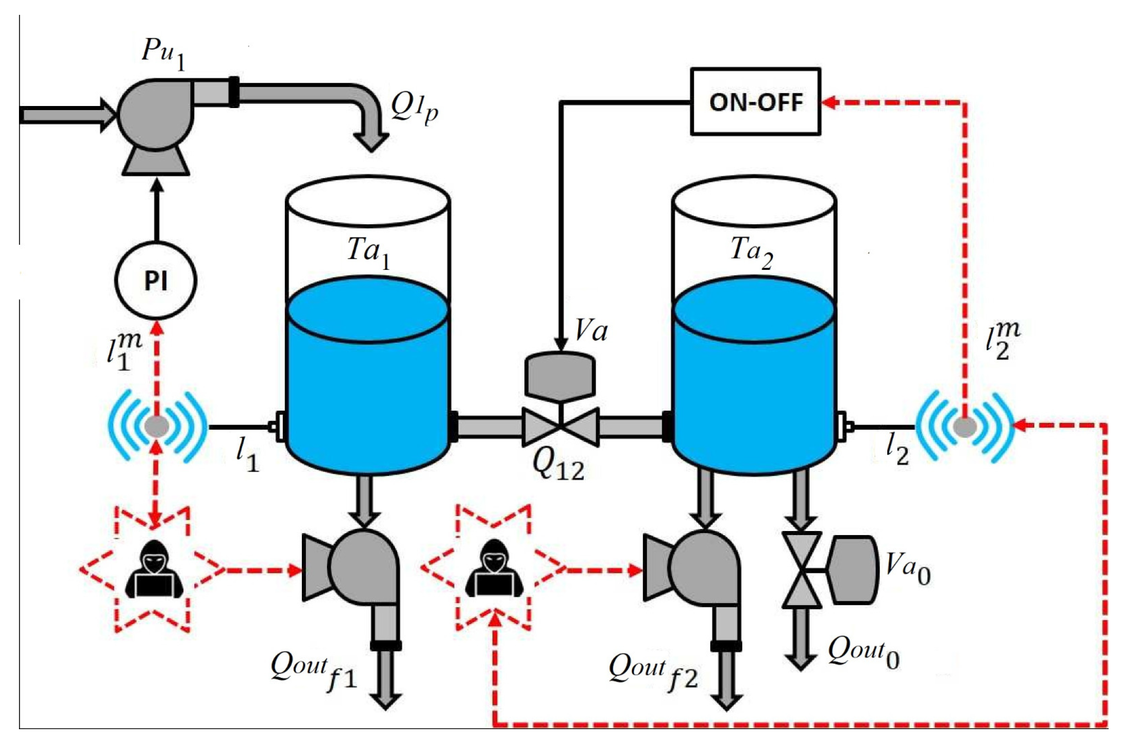
This type of system is characteristic of process industries such as petrochemicals, energy, and mining. The system consists of two tanks linked together by a pipe fitted with a valve $V{a}_b$ managed by an ON–OFF controller (see Figure 11) [35]. Pump $P{u}_1$ is managed by the control signal $U{1}_p$ from a Proportional Integral (PI) controller, and feeds Tank 1 ($T{a}_1$). Tank 2 ($T{a}_2$) has a manual valve $V{a}_0$ installed at the outlet.

Table 2. Variables of the plant.

Symbol	Description
$Q{1}_p$	Inflow to $T{a}_1$
$l_1$	Water level in $T{a}_1$
$l_2$	Water level in $T{a}_2$
$Qou{t}_0$	Outflow to consumers
$Qou{t}_{f1}$	Outflow at $T{a}_1$
$Qou{t}_{f2}$	Outflow at $T{a}_2$

shows the set of measured variables of the plant.

In this system, the following operating states were considered:

• NOC: Normal operating condition.
• F-1: This scenario corresponds to Fault 1 due to a water leak in Tank 1 ($T_1$) at a constant flow $Q_{f1}$ = ${10}^{-4}$ m³/s in the time interval 40 s $\ge t\le$ 80 s.
• A-1: This scenario corresponds to Attack 1, involving water theft in tank $T_1$ with a hidden signal added to the $h_1^m$ level reading (deception attack). In this case, the attacker withdraws a steady flow rate of $Q_{f1}$ = ${10}^{-4}$ m³/s via the pump during the period 40 s $\ge t\le$ 80 s. To conceal the theft, they inject a spoofed signal into the level sensor output at $T_1$. As a result, the measured level at $T_1$ appears constant and the PI controller continues operating normally, producing a control output $U_p^m$ similar to the NOC.
• F-2: This scenario corresponds to Fault 2 due to a water leak in Tank 2 ($T_2$) at a constant flow $Q_{f2}$ = ${10}^{-4}$ m³/s in the time interval 40 s $\ge t\le$ 80 s.
• A-2: In this scenario, the attacker initiates water theft when the system has reached a steady state. Prior to launching the attack, the attacker records sensor measurements even if water has already been illicitly extracted from the tanks. Subsequently, during the execution phase, the attacker continues to steal water while substituting the actual sensor data with the previously recorded measurements, constituting a replay attack. Specifically, water is withdrawn during the time interval 160 s $\ge t\le$ 200 s, while the sensor readings captured at t = 50 s (prior to the attack) are replayed to deceive the controller.

4.2.2. Design of Experiments

Offline: Training Stage

To conduct the training phase, 200 observations were taken from each operating state (NOC, Faults, and Attacks). The F-2 and A-2 patterns were not included in the training dataset. The aim was to assess the algorithm’s ability to identify and locate new events during the online phase. For this reason, two experiments were conducted during the training phase:

• Experiment 1: F-2 was not considered during training. The training database (TDB1) was made up of the following pattern: NC, F-1, A-1, A-2.
• Experiment 2: A-2 was not considered during training. The training database (TDB2) was made up of the following pattern: NC, F-1, A-1, F-2.

For both experiments, the MLP network was built with four neurons in the output layer (four classes) and a softmax activation function. The same hyperparameters were used according to Table 1. To determine the parameter $Nn$ using the DE algorithm, the same control parameters described in Section 4.1.1 were used. In this case, the search space is $1\le N{n}^l\le 20$. In this case, five neighbors (h = 5) were used for the LOF algorithm.

Online: Recognition Stage

In the online phase, forty observations were used for each class. In addition, fifty new samples (ten for each operating state) were added to this data set, distributed evenly across classes, to represent potential outliers. Outliers were generated as values outside the measurement range for each variable.

To validate the online recognition phase, three variants were considered for each experiment carried out in the training. In all scenarios, fifty observations were used to simulate the sequential acquisition of data in an online setting.

Experiment 1: TDB1

• Scenario 1: Fifty samples were utilized, with forty belonging to NOC and ten being outliers. The aim was to assess the system’s ability to accurately classify normal functioning and its ability to detect several samples that represent outliers as SAS.
• Scenario 2: Ten samples from F-1 and forty outliers that did not constitute a class were used. The aim was to analyze the system’s accuracy in classifying the F-1 fault and its capacity to detect multiple outliers, such as SAS points which do not form a new class due to their low density.
• Scenario 3: Forty samples from unknown event (Fault F-2) and ten outliers were used. The aim was to analyze the appropriate classification of these samples as SAS and the capacity to detect which of these values formed a new class (new fault).

Experiment 2: TDB2

• Scenario 1: Fifty samples were utilized, with forty belonging to A-1 and ten being outliers. The aim was to evaluate the system’s ability to accurately classify attack A-1 and its ability to detect several samples that represent outliers as SAS.
• Scenario 2: Ten samples from F-2 and forty outliers that did not constitute a class were used. The aim was to analyze the system’s accuracy in classifying fault F-2 and its capacity to detect multiple outliers, such as SAS points which do not form a new class due to their low density.
• Scenario 3: Forty samples from an unknown event (Attack A-2) and ten outliers were used. The aim was to analyze the appropriate classification of these samples as SAS and the ability to detect which of these values conformed to a new class (new attack).

4.2.3. Analysis and Discussion of Results

Offline: Training Stage

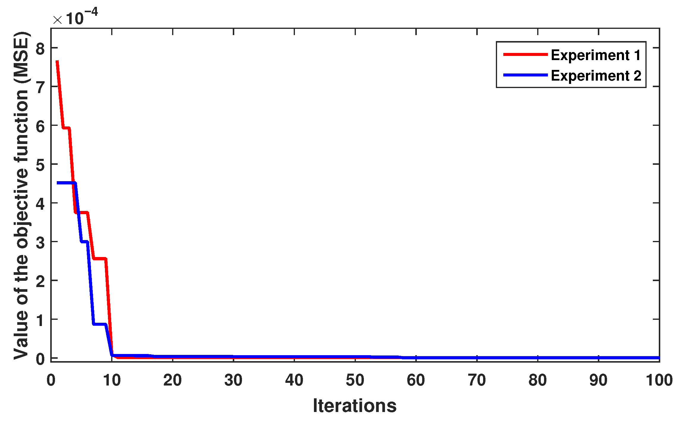
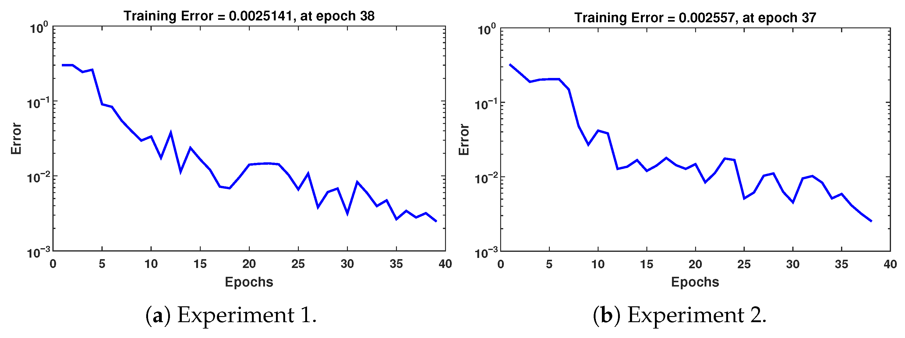
For both experiments, the performance of the objective function (MSE) is illustrated in Figure 12, again demonstrating the rapid convergence of the DE algorithm. In both experiments, the best parameter was $N{n}^1$ = 10, obtained in iteration 10. The training error achieved by the MLP network with DE-estimated parameters is shown in Figure 13, while Figure 14 shows the confusion matrices during the training phase for the two experiments.

Online: Recognition Stage

Under the premise of quickly detecting a new event, fifty samples were considered for evaluation. Therefore, a time window $k=50$, equivalent to 50 s, was considered. Furthermore, to define an appropriate level for most of the samples classified as unknown events, it was decided to use a decision threshold of $Li=60\%$. It is important to highlight that the selection of these parameters responds to the type of process and the opinions of the specialists.

Table 3. Confusion matrix for online classification: LOF-MLP.

LOF-MLP
	TDB1-Scenario 1			TDB1-Scenario 2			TDB1-Scenario 3	TDB2-Scenario 1			TDB2-Scenario 2			TDB2-Scenario 3
	NOC	SAS	AVE	F-1	SAS	AVE	SAS	A-1	SAS	AVE	F-2	SAS	AVE	SAS
NOC	40	0		0	0		0	2	0		0	0		1
F-1	0	0		10	0		0	0	0		0	0		0
A-1	0	0		0	1		0	38	0		0	1		0
A-2/F-2	0	0		0	1		0	0	0		10	0		0
O	0	10		0	38		50	0	10		0	39		49
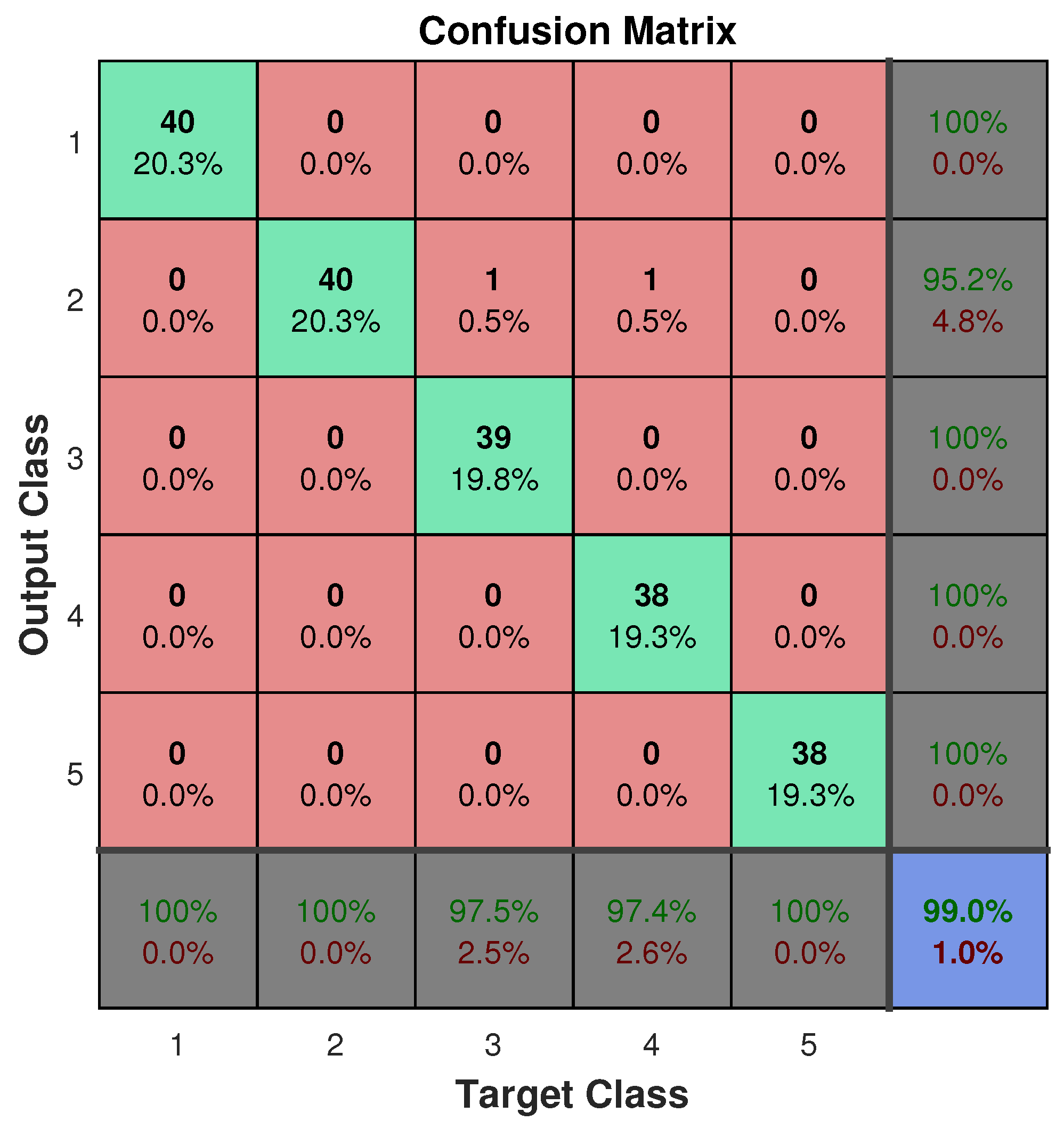
TA (%)	100	100	100	100	95.00	96.00	100	95.00	100	96.00	100	97.50	98.00	98.00

and

Table 4. Confusion matrix for online detection of new events: LOF-Algorithm.

LOF-Algorithm
	TDB1-Scenario 2	TDB1-Scenario 3			TDB2-Scenario 2	TDB2-Scenario 3
	SAS	NE	O	AVE	SAS	NE	O	AVE
NE	0	39	0		0	38	0
O	38	1	10		39	1	10
TA (%)	100	97.50	100	98.00	100	97.44	100	97.96

show the confusion matrices for the experiments described in the previous section. We considered the states NOC, F-1, A-1, F-2, A-2, and New Event (NE), along with the Outliers (O) class. The main diagonal of the confusion matrix indicates the number of samples accurately identified or classified, while the off-diagonal values reflect misclassifications. The classification accuracy for each class and total can be computed using the information of the confusion matrix. The last row exhibits the Average Accuracy (AVE) across all classes.

Analysis of Results.

As seen in Table 3, satisfactory results were obtained thanks to accurate classification of both the NOC class and the outliers. In Scenario 1 (TDB1), the LOF algorithm classifies the ten samples as $SAS$, then $AOP<Li$; therefore, the density of the set of $SAS$ was not evaluated. For Scenario 2 (TDB1), it is shown that the online algorithm achieved satisfactory results in identifying ten samples from the F-1 fault and the forty outliers. In this scenario, the LOF algorithm classifies 38 observations as $SAS$, meaning that $AOP>Li$, then evaluates the density of the set of SAS. The two outliers identified as known classes are analyzed by the MLP algorithm and classified into classes A-1 and A-2. In Scenario 3 (TDB1), forty samples belonging to a new event (Fault F-2) and ten outlier observations are evaluated and classified over fifty sample periods. In this scenario, the LOF algorithm classifies fifty observations as $SAS$; thus, $AOP>Li$, meaning that the set of outliers must be analyzed.

Considering Scenario 1 (TDB2), Table 3 displays the obtained results. In this scenario, satisfactory results are obtained thanks to accurate classification of attack A-1 and the outliers. For Scenario 2 (TDB2), the ten samples of fault F-2 and the forty outliers are successfully identified. In this case, the LOF algorithm classifies 39 observations as $SAS$; thus, $AOP>Li$, and the density of the set of $SAS$ must be evaluated. The outlier identified as a known class is analyzed by the MLP algorithm and classified into the A-1 class.

In Scenario 3 (TDB2), the classification of forty samples belonging to a new event (Attack A-2) and ten outliers is evident. In this case, the LOF algorithm classifies 49 observations as $SAS$; thus, $AOP>Li$, meaning that the set of outliers must be analyzed. The $SAS$ identified as a known class is analyzed by the MLP algorithm and classified into the NOC class.

For Scenario 2 (TDB1), Table 4 shows the evaluation results of the 38 samples identified as $SAS$. In this case, the density-based LOF algorithm must determine which $SAS$ items in the set are classified as either a new event or as outliers. In this analysis, the LOF algorithm is used to identify a single new class, where the set of $SAS$ represents the outliers. The next crucial step requires experts to evaluate these results and decide whether a new event implies a new attack or fault pattern. As can be seen, all observations are identified as outliers; therefore, they are removed and the $AS$ and S counters are reset.

For Scenario 3 (TDB1), Table 4 shows the results after implementing the LOF algorithm to classify the set of $SAS$ as outliers or as a new event. In this case, the presence of a new event (Fault F-2) is clearly evident. After identifying a new class, experts must characterize the pattern and update the historical database. This crucial step allows the condition monitoring system algorithms to be retrained, thereby integrating the new pattern.

For Scenario 2 (TDB2), the evaluation results for the 39 samples identified as $SAS$ are shown. In this case, all observations are identified as outliers; therefore, they are deleted and the $AS$ and S counters are reset. In Scenario 3 (TDB2), Table 4 presents the results after implementing the density-based LOF algorithm to classify the 49 $SAS$ as either outliers or as a new event. It can be seen that the presence of a new event (Attack A-2) is evident.

Figure 15 shows the results after the new events (fault F-2 and attack A-2) are identified and updated in the training database.

Table 5. Performance in the online classification stage.

	Precision (%)	Recall (%)	F1-Score (%)
NOC	100	100	100
F-1	100	95.24	97.54
A-1	97.50	100	98.73
F-2	97.40	100	98.68
A-2	100	100	100

shows the performance in the online classification stage. For each operating state analyzed, high precision (percentage of accurate predictions among all positive predictions) is evident, always maintaining values above 97%. Recall (percentage of positive labels that the classifier correctly predicted to be positive) shows satisfactory performance, achieving 95.24% for F-1 and 100% for the remaining classes. Finally, the F1 score is always above 97 %, offering an excellent balance between the previous metrics.

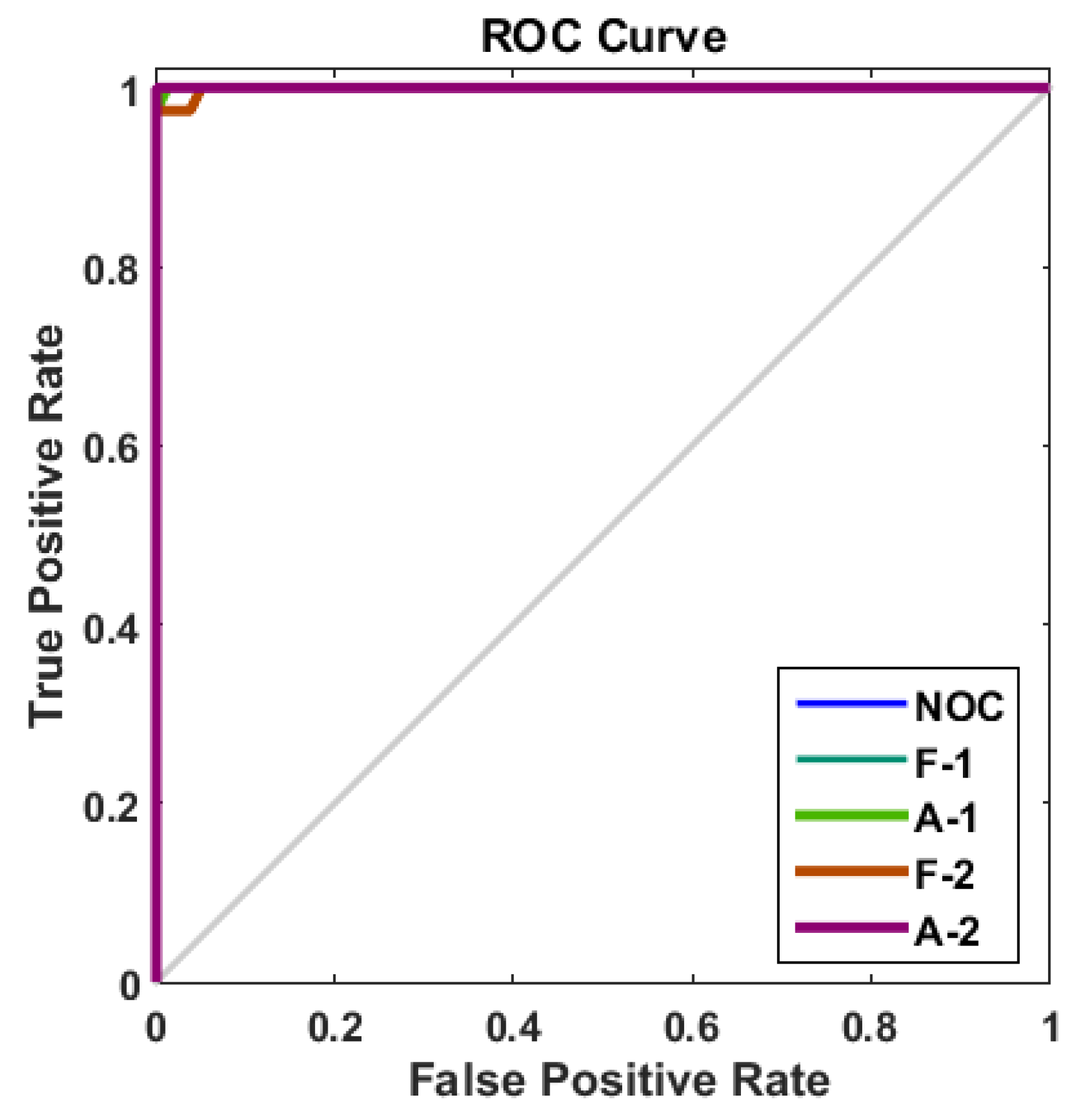
In addition, the Receiver Operating Characteristic (ROC) curve shown in Figure 16 demonstrates satisfactory performance in classifying the analyzed operating states. It can be seen that the ROC curve tends towards the upper left corner, indicating a high True Positive Rate (TPR) close to 1 and low False Positive Rate (FPR) close to 0.

4.2.4. Comparison with Other Machine Learning Tools

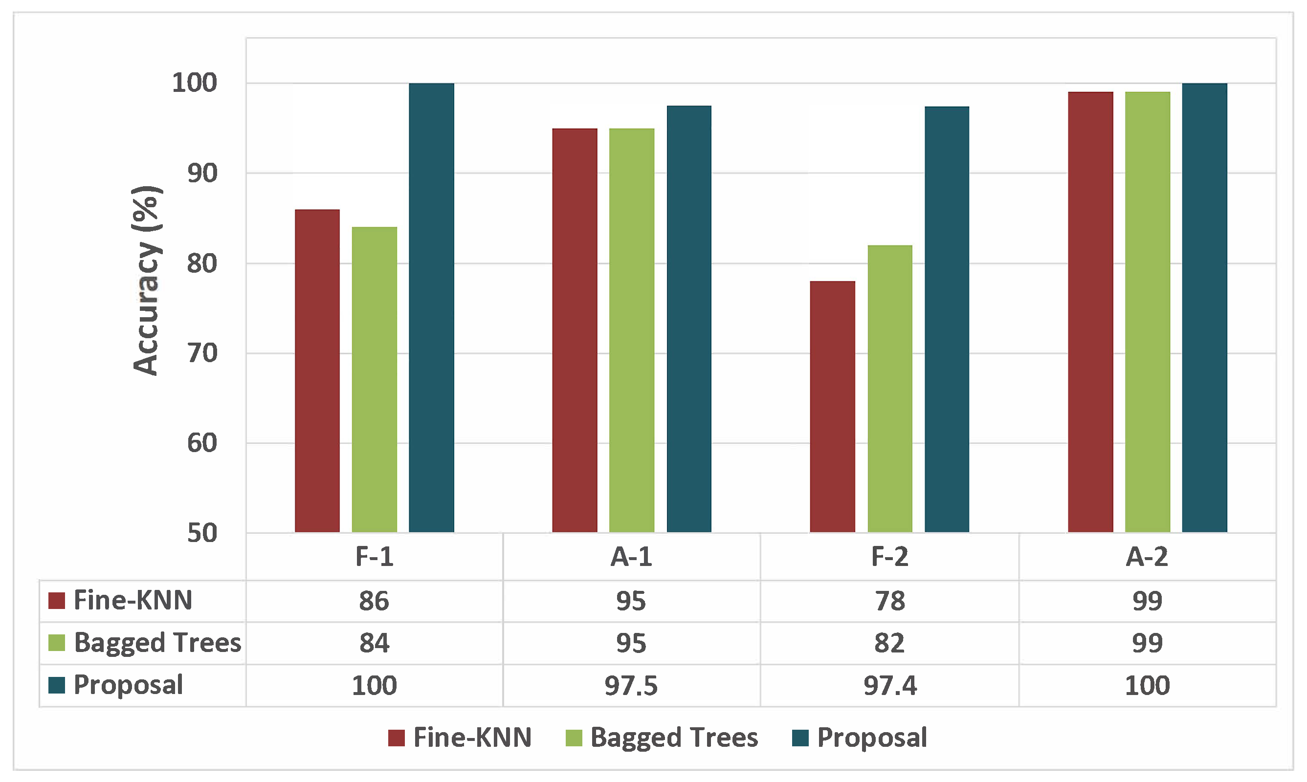
The results presented in Figure 15 using the LOF-MLP algorithm were compared to those obtained with other machine learning tools described in [36]. The algorithms included in the comparison are Boosted Trees, Bagged Trees, Medium Tree, Fine Tree, Coarse Tree, Subspace Discriminant, Linear Discriminant, Fine KNN, Medium KNN, and Coarse KNN.

The results shown in Figure 17 reflect the overall classification, confirming the superior performance of the scheme proposed in this work. A comparison with the best methods used in [36] is shown in Figure 18. The accuracy values in the classification of each operating state (without considering the NOC) reflect the excellent performance of the proposal presented in this work.

5. Conclusions

This work presents a novel two-stage architecture for condition monitoring in industrial plants. The effective combination of computational intelligence tools inside the proposed architecture achieves excellent results. In the first stage, a machine learning model with optimized parameters is trained offline. In the second stage, which takes place online, a detection mechanism and a classification system are effectively combined. The implemented detection mechanism separates the received observations into two large groups based on whether or not they belong to a known pattern. Observations that are considered to not belong to known patterns are systematically evaluated in order to identify unknown patterns and eliminate outliers which affect the classification system. Identified unknown patterns are characterized by experts and added to the training database, ensuring incremental learning and the resilience of the proposed strategy. Observations deemed to fit known patterns are classified by the machine learning model using the optimized parameters trained in the first stage. This model proves to be highly effective in identifying classes corresponding to faults, cyberattacks, and normal operating mode. The absence of observations belonging to unknown classes and outliers in the final classification process is a key element in the outstanding performance results obtained by the proposed architecture.

The implementation of the proposed strategy was achieved using a Multilayer Perceptron Neural Network as a Machine Learning model, the Differential Evolution algorithm to optimize the hyperparameters of the previous model, and the Local Outlier Factor algorithm in the mechanism for detecting unknown patterns and eliminating outliers.

The use of ML tools enables efficient handling of large and noisy sets of observations, which improves classification performance even when fault and attack categories overlap. This integration of commonly independent operations into an integrated approach is a major scientific advancement, fostering better cooperation between Operational Technology (OT) and Information Technology (IT) teams. It also boosts system reliability, strengthens security, and lowers computational complexity, offering a practical solution for today’s industrial settings.

The proposed framework was validated using the two-tank process benchmark, a characteristic system of process industries such as petrochemicals, energy, and mining. The results demonstrate an accuracy of over 99% and superior robustness compared to other machine learning algorithms. These results highlight the potential of combining fault diagnosis and cybersecurity in a unified architecture, thereby contributing to resilient and intelligent systems that meet the demands of Industry 4.0/5.0.

Notwithstanding the above, this work’s supervised learning framework is constrained by its dependence on labeled data, which are often unavailable in industrial settings, as well as by the inherent lack of interpretability of neural network models, which impedes analysis of feature importance. To overcome these limitations, future work will explore unsupervised learning techniques, such as those presented in [37,38] for real-time embedded systems. This shift will leverage unlabeled data to identify complex patterns, thereby enhancing the performance of fault and cyberattack detection and localization. On the other hand, it would be also interesting to explore deep learning approaches that incorporate physics-informed neural networks, as presented in [39], where physical knowledge is integrated into input preparation, model construction, and output specification. This could result in a more interpretable and robust model.

References

1. Macas, M.; Wu, C.; Fuertes, W. A survey on deep learning for cybersecurity: Progress, challenges, and opportunities. Comput. Netw. 2022, 212, 109032. [Google Scholar] [CrossRef]
2. Bashendy, M.; Tantawy, A.; Erradi, A. Intrusion response systems for cyber-physical systems: A comprehensive survey. Comput. Secur. 2023, 124, 102984. [Google Scholar] [CrossRef]
3. Lucchese, M.; Salerno, G.; Pugliese, A. A Digital Twin-Based Approach for Detecting Cyber–Physical Attacks in ICS Using Knowledge Discovery. Appl. Sci. 2024, 14, 8665. [Google Scholar] [CrossRef]
4. Azzam, M.; Pasquale, L.; Provan, G.; Nuseibeh, B. Forensic readiness of industrial control systems under stealthy attacks. Comput. Secur. 2023, 125, 103010. [Google Scholar] [CrossRef]
5. Committee on National Security Systems (cnss) Glossary, cnssi 4009. Available online: https://www.niap-ccevs.org/ (accessed on 10 June 2025).
6. Perales Gómez, A.L.; Fernández Maimó, L.; Huertas Celdrán, A.; García Clemente, F.J. VAASI: Crafting valid and abnormal adversarial samples for anomaly detection systems in industrial scenarios. JISA 2023, 79, 103647. [Google Scholar] [CrossRef]
7. Anthi, E.; Williams, L.; Rhode, M.; Burnap, P.; Wedgbury, A. Adversarial attacks on machine learning cybersecurity defences in industrial control systems. JISA 2021, 58, 102717. [Google Scholar] [CrossRef]
8. Garcia, J.; Rios-Colque, L.; Peña, A.; Rojas, L. Condition Monitoring and Predictive Maintenance in Industrial Equipment: An NLP-Assisted Review of Signal Processing, Hybrid Models, and Implementation Challenges. Appl. Sci. 2025, 15, 5465. [Google Scholar] [CrossRef]
9. Kravchik, M.; Demetrio, L.; Biggio, L.; Shabtai, A. Practical evaluation of poisoning attacks on online anomaly detectors in industrial control system. Comput. Secur. 2022, 122, 1–20. [Google Scholar] [CrossRef]
10. Doing, D.; Han, Q.; Xiang, Y.; Zhang, X. New features for fault diagnosis by supervised classification. IEEE Trans. Instrum. Meas. 2021, 70, 1–15. [Google Scholar]
11. Lundgren, A.; Jung, D. Data-driven fault diagnosis analysis and open-set classification of time-series data. Control Eng. Pract. 2022, 121, 105006. [Google Scholar] [CrossRef]
12. Ahmad, R.; Alsmadi, I.; Alhamdani, W.; Tawalbeh, L. A Deep Learning Ensemble Approach to Detecting Unknown Network Attacks. JISA 2022, 67, 103196. [Google Scholar] [CrossRef]
13. Huang, H.; Li, T.; Ding, Y.; Li, B.; Liu, A. An artificial immunity based intrusion detection system for unknown cyberattacks. Appl. Soft Comput. 2023, 148, 110875. [Google Scholar] [CrossRef]
14. Khan, N.A.; Sulaiman, M.; Lu, B. Predictive insights into nonlinear nanofluid flow in rotating systems: A machine learning approach. Eng. Comput. 2025, 41, 179–196. [Google Scholar] [CrossRef]
15. Said, N.; Mansouri, M.; Al Hmouz, R.; Khedher, A. Deep Learning Techniques for Fault Diagnosis in Interconnected Systems: A Comprehensive Review and Future Directions. Appl. Sci. 2025, 15, 6263. [Google Scholar] [CrossRef]
16. Rodríguez-Ramos, A.; Bernal de Lázaro, J.M.; Silva Neto, A.; Llanes Santiago, O. Fault detection using kernel computational intelligence algorithm. In Computational Intelligence, Optimization and Inverse Problems with Applications in Engineering; Platt, G., Yang, X.S., Silva Neto, A., Eds.; Springer: Berlin/Heidelberg, Germany, 2019; pp. 63–75. [Google Scholar]
17. Shaukat, K.; Luo, S.; Varadharajan, V. A novel method for improving the robustness of deep learning-based malware detectors against adversarial attacks. Eng. Appl. Artif. Intell. 2022, 116, 105461. [Google Scholar] [CrossRef]
18. Kok, A.; Martinetti, A.; Braaksma, J. The Impact of Integrating Information Technology With Operational Technology in Physical Assets: A Literature Review. IEEE Access 2024, 12, 111832–111845. [Google Scholar] [CrossRef]
19. Jeffrey, N.; Tan, Q.; Villar, J.R. A hybrid methodology for anomaly detection in Cyber–Physical Systems. Neurocomputing 2024, 568, 127068. [Google Scholar] [CrossRef]
20. Ma, F.; Ji, C.; Rao, J.; Han, C.; Wang, J.; Sun, W. A cyber-attack detection based on time-delay mutual information analysis. Process Saf. Environ. Prot. 2025, 200, 107361. [Google Scholar] [CrossRef]
21. Taheri, M.; Khorasani, K.; Shames, I.; Meskin, N. Cyberattack and machine-induced fault detection and isolation methodologies for cyber-physical systems. IEEE Trans. Control Syst. Technol. 2024, 32, 502–517. [Google Scholar] [CrossRef]
22. Müller, N.; Bao, K.; Matthes, J.; Heussen, K. Cyphers: A cyberphysical event reasoning system providing real-time situational awareness for attack and fault response. Comput. Ind. 2023, 151, 103982. [Google Scholar]
23. Amin, M.T.; Khan, F.; Halim, S.Z.; Pistikopoulos, S. A holistic framework for process safety and security analysis. Comput. Chem. Eng. 2022, 165, 107963. [Google Scholar]
24. Syfert, M.; Ordys, A.; Koscielny, J.M.; Wnuk, P.; Mozaryn, J.; Kukiełka, K. Integrated approach to diagnostics of failures and cyber-attacks in industrial control systems. Energies 2022, 15, 6212. [Google Scholar] [CrossRef]
25. Elsisi, M.; Tran, M.Q.; Mahmoud, K.; Mansour, D.E.; Lehtonen, M.; Darwish, M.M. Effective iot-based deep learning platform for online fault diagnosis of power transformers against cyber-attacks and data uncertainties. Measurement 2022, 190, 110686. [Google Scholar] [CrossRef]
26. Breunig, M.M.; Kriegel, H.-P.; Ng, R.T.; Sander, J. LOF: Identifying density-based local outliers. In Proceedings of the 2000 ACM SIGMOD International Conference on Management of Data, Dallas, TX, USA, 15–18 May 2000; pp. 93–104. [Google Scholar]
27. Rodríguez-Ramos, A.; Silva-Neto, A.J.; Llanes-Santiago, O. An approach to fault diagnosis with online detection of novel faults using fuzzy clustering tools. Expert Syst. Appl. 2018, 113, 200–212. [Google Scholar] [CrossRef]
28. Tuptuk, N.; Hailes, S. Identifying vulnerabilities of industrial control systems using evolutionary multiobjective optimisation. Comput. Secur. 2024, 137, 103593. [Google Scholar] [CrossRef]
29. Rodríguez-Ramos, A.; Bernal de Lázaro, J.; Prieto-Moreno, A.; Silva Neto, A.; Llanes-Santiago, O. An approach to robust fault diagnosis in mechanical systems using computational intelligence. JIM 2019, 30, 1601–1615. [Google Scholar] [CrossRef]
30. Bilal; Pant, M.; Zaheer, H.; García-Hernández, L.; Abraham, A. Differential Evolution: A review of more than two decades of research. Eng. Appl. Artif. Intell. 2020, 90, 103479. [Google Scholar] [CrossRef]
31. Kilic, V.N.; Essiz, E.S. K-Salp Swarm Anomaly Detection (K-SAD): A novel clustering and threshold-based approach for cybersecurity applications. Comput. Secur. 2025, 151, 104325. [Google Scholar] [CrossRef]
32. Adesh, A.; Shobha, G.; Shetty, J.; Xu, L. Local outlier factor for anomaly detection in HPCC systems. J. Parallel Distrib. Comput. 2024, 192, 104923. [Google Scholar] [CrossRef]
33. Mattera, G.; Mattera, F.; Vespoli, S.; Salatiello, E. Anomaly detection in manufacturing systems with temporal networks and unsupervised machine learning. CAIE 2025, 203, 111023. [Google Scholar] [CrossRef]
34. Kaur, P.; Soni, A.; Gosain, A. Robust kernelized approach to clustering by incorporating new distance measure. Eng. Appl. Artif. Intell. 2013, 26, 833–847. [Google Scholar] [CrossRef]
35. Quevedo, J.; Sánchez, H.; Rotondo, D.; Escobet, T.; Puig, V. A two-tank benchmarkfor detection and isolation of cyber-attacks. IFAC Pap. OnLine 2018, 51, 770–775. [Google Scholar] [CrossRef]
36. Chanthery, E.; Audine, S. Diagnosis approaches for detection and isolation of cyber attacks and faults on a two-tank system. In Proceedings of the 30th International Workshop on Principles of Diagnosis DX’19, Klagenfurt, Austria, 11–13 November 2019. hal-02439489. [Google Scholar]
37. Rivera Torres, P.J.; Gershenson García, C.; Sánchez Puig, M.F.; Kanaan Izquierdo, S. Reinforcement Learning with Probabilistic Boolean Network Models of Smart Grid Devices. Complexity 2022, 265241. [Google Scholar] [CrossRef]
38. Rivera Torres, P.J.; Gershenson García, C.; Sánchez Puig, M.F.; Kanaan Izquierdo, S. Reinforcement Learning with Probabilistic Boolean Networks in Smart Grid Models. In Proceedings of the 19th Latin American Control Congress; Springer: Cham, Switzerland, 2022; pp. 215–224. [Google Scholar]
39. Yin, C.; Li, Y.; Wang, Y.; Dong, Y. Physics-guided degradation trajectory modeling for remaining useful life prediction of rolling bearings. MSSP 2025, 224, 112192. [Google Scholar] [CrossRef]
Figure 1. General MLP architecture for condition monitoring systems.
Processes 13 02984 g001
Figure 2. Local Outlier Factor (LOF) process: (a) determine the h-value; (b) calculate the RD; (c) calculate the LRD; (d) calculate the LOF score for each data point.
Processes 13 02984 g002
Figure 3. Proposal of CM scheme with online identification of unknown event.
Processes 13 02984 g003
Figure 4. Diamond dataset.
Processes 13 02984 g004
Figure 5. Objective function value.
Processes 13 02984 g005
Figure 6. Training error for the MLP-DE algorithm.
Processes 13 02984 g006
Figure 7. Results of training using the LOF algorithm.
Processes 13 02984 g007
Figure 8. Results of the online analysis stage (Experiment 1).
Processes 13 02984 g008
Figure 9. Results of the online analysis stage (Experiment 2).
Processes 13 02984 g009
Figure 10. Results of the online analysis stage (Experiment 3).
Processes 13 02984 g010
Figure 11. Scheme of the two-tank process.
Processes 13 02984 g011
Figure 12. Objective function value.
Processes 13 02984 g012
Figure 13. Training error for the MLP-DE algorithm.
Processes 13 02984 g013
Figure 14. Confusion matrix for the training stage (1, 2, 3, 4: 200).
Processes 13 02984 g014
Figure 15. Confusion matrix: Online stage (1: NOC; 2: F-1; 3: A-1; 4: F-2; 5: A-2).
Processes 13 02984 g015
Figure 16. ROC curve for the online stage.
Processes 13 02984 g016
Figure 17. Overall classification results.
Processes 13 02984 g017
Figure 18. Classification results for F-1, A-1, F-2, and A-2.
Processes 13 02984 g018