Abstract
Efficient scheduling is critical for the success of any organization. Researchers have proposed numerous strategies for addressing various scheduling problems. The hybrid flow shop (HFS) scheduling is a complex and NP-hard problem that arises in many manufacturing and service industries. This work introduces an optimization technique that utilizes atomic orbitals to address issues in HFS scheduling. Our objective is to reduce makespan (Cmax). Makespan minimization is critical for improving productivity and resource utilization. The standard atomic orbital search optimization algorithm (AOSOA) is hybridized with constructive heuristics to enhance solution quality. The scheduling problem of an electrical panel board manufacturing industry is solved using the hybrid AOSOA (HAOSOA). The results were better than those previously reported. A variety of random test situations of varying sizes and configurations were devised to assess the efficacy of the suggested algorithm. The proposed algorithm’s outcomes were compared against well-known algorithms discussed in the literature. Friedman and Wilcoxon test results indicate that the proposed methodology improves the solution quality in each test instance compared to all the metaheuristics used for comparison. The performance of the proposed algorithm is also evaluated using benchmark problems from the literature. In the first test, the algorithm has a rank value of 1, indicating it performs better than each of the comparing algorithms. In the second test, it is able to find the best makespan for 65 of the 77 problems.
1. Introduction
Scheduling is widely used in different domains, including manufacturing, services management, computing, airline routing, aircraft maintenance, hospitals, timetabling for schools and universities, supermarkets, and transportation. For example, in manufacturing, scarce resources are assigned to jobs, and then these assigned jobs are sequenced according to each resource. Various types of scheduling environments have been given in the academic field [1]. Due to its significance in both theoretical and practical contexts, the hybrid flow shop (HFS) has recently garnered much attention. The intractable nature of this problem, characterized by its strong non-deterministic polynomial-time hard (NP-hard) property, renders the utilization of exact methods for problems impractical, even in the context of relatively modest problem sizes. Consequently, researchers have explored numerous heuristics and metaheuristics methodologies to solve these problems. On the other hand, the HFS environment can be representative of real-world industries such as electronics, furniture manufacturing, and other production environments [2,3]. Hence, in this study, an HFS problem is analyzed to address the key technical challenges in finding optimal solutions.
1.1. Hybrid Flow Shop Scheduling Problems
In essence, an HFS comprises a flow shop, along with parallel machine environments, and includes multiple stages, each with parallel machines and a task that necessitates the simultaneous completion of both components. To optimize performance, Allaoui and Artiba [4] investigated a 2-stage HFS schedule allocation with m machines incorporated following the initial phase. Their objective was to identify the most feasible minimal makespan. They opted for a branch-and-bound strategy after evaluating the pertinent model and the likelihood of machine failure. However, the branch-and-bound method can only be used to solve small problems. Hence, to tackle the HFS scheduling problems of medium and large sizes, metaheuristics may be used. Jabbarizadeh et al. [5] developed various heuristics and metaheuristics to reduce the makespan in a hybrid flexible flow shop (FFS) scheduling system characterized by restricted machine availability and setup times dependent on task sequence. Luo et al. [6] introduced a genetic algorithm (GA) based solution approach to solve problems in a metalworking company under the makespan criterion. The metalworking procedure comprises two separate stages. The early phase involves multiple gadgets, but the subsequent stage demands only one piece of equipment. They considered batching operations, a blocking environment, machine unavailability, and sequence-dependent setup time (SDST) in their research work. Zandieh and Gholami [7] analyzed the HFS scheduling problems under SDST and machine breakdowns for minimizing the projected makespan. They introduced an immune algorithm (IA) to handle the proposed model.
Behnamian and Ghomi [8] developed a hybrid GA/VNS (variable neighborhood search) approach to address HFS scheduling challenges, aiming to minimize overall resource allocation costs and duration. Their research focused on processing durations that varied according to the available technology and resources. From this work, it is understood that the performance of metaheuristics could be improved by hybridizing them with local search techniques or heuristics. Choi and Wang [9] devised an innovative decomposition-based approach to minimize the makespan with probabilistic processing durations in a flexible flow shop. Kianfar et al. [10] analyzed the FFS scheduling problems with SDST, where they considered the jobs’ arrival time to be uncertain and dynamic to minimize the average job delay using a hybrid GA. Mirabi et al. [11] examined a two-stage HFS scenario, where a solitary machine is used in the initial phase and numerous identical machines operate simultaneously in the subsequent phase, in the event of machine failures. However, two-stage scheduling problems are practically insignificant, as real industrial scheduling problems typically involve multiple stages. Wang et al. [12] employed a cluster-based scheduling technique to address the HFS problem, which involves fluctuating processing durations and machine failures. Ebrahimi et al. [13] investigated the HFS to reduce makespan and total delay, considering the different setup durations of families based on their sequence of occurrence. Wang and Choi [14] developed a holonic decomposition-based method to rectify the changeable flow shop schedule with modifiable processing durations. They achieved this by subjecting the program to multiple random evaluations.
Wang et al. [15] proposed a multi-objective problem in a two-stage HFS environment with maintenance. In Liu et al. [16], HFS is analyzed with the focus on working conditions. Multi-skilled workers and fatigue factors are incorporated within scheduling. Maciel et al. [17] designed a hybrid GA for blocking machine and SDST in a hybrid Flow Shop Scheduling Problem (FSSP) under makespan. In Fu et al. [18], a stochastic HFS is analyzed, which more closely resembles real-world applications. Researchers are investigating artificial bee colony methods to minimize makespan. In a preliminary phase of the hot-cold casting process, Wang et al. [19] addressed the HFS problem using batch processing equipment. Yu et al. [20] investigated the hybrid flow shop setting utilizing the total tardiness criterion. Production assembly and worker resources are also taken into account in the model. Zhang et al. [21] employed a hybrid approach integrating Particle Swarm Optimization (PSO) and Q-learning to address the energy-efficient Hybrid Flow Shop (HFS) problem. Their methodology is to maximize energy efficiency for both energy consumption and makespan. Geetha et al. [22] analyzed the carbon emission problem under the HFS environment. A pigeon-inspired optimization algorithm is selected to handle the problem. From the above literature review, it is evident that metaheuristics perform well in solving HFS scheduling problems to minimize makespan. Hence, in this work, an attempt is made to solve the HFS scheduling problems using a newly developed metaheuristics algorithm.
1.2. Atomic Orbital Search Optimization Algorithm (AOSOA)
Authors developed an improved Atomic orbital search optimization algorithm (AOSOA) using a global search approach that employs a numerical optimization method to harness its effective exploration capability for feature selection in machine learning methods in [23]. The opposite-based learning approach augments the initial population, accelerating convergence to the optimal result. A dynamic photon rate strikes an equilibrium between exploration and exploitation. The successive backward selection strategy improves the quality of the optimal findings. To control the unknown parameters of a solar cell, AOSOA is proposed. The model is tested for various solar cell design problems. Based on comparisons with different algorithms, AOSOA appears to produce better solution values [24]. In [25], AOSOA is introduced using different benchmark problems and engineering design problems. Statistical analysis shows that the new approach has better solution quality than the comparison algorithms. Different truss structures are investigated to assess the efficiency of the AOSOA in solving truss optimization problems. A comparative analysis of the AOSOA with those of other methods documented in the literature reveals the AOSOA to be effective in addressing complex design problems, as evidenced by its notable capacity for weight reduction [26]. The study [27] examines various constrained design problems from different engineering fields to evaluate AOSOA. The findings of AOSOA for solving these engineering design problems were assessed, and AOSOA exhibited superior performance in most cases.
A multi-objective approach has been developed for the AOSOA [28]. In the study, a range of metrics is employed to evaluate different benchmark and engineering design problems. The multi-objective AOSOA often leads to better solutions. The AOSOA was used in the project scheduling of a dam construction [29]. Considering the necessity to minimize time, cost, risk, and ensure the highest quality, AOSOA is proposed to solve this issue. The outcomes of this assessment are then evaluated against various metaheuristic methods. The findings indicated that this approach could lessen the time and cost of the dam project. The AOSOA has been revised to incorporate a dynamic, opposite-based learning mechanism. This facilitates the examination of the search domain for many potential solutions to the feature selection problem [30].
A variety of algorithms were employed for comparative analysis. The modified AOSOA, based on statistical analysis, demonstrates superior performance. The practical and efficient extraction of solar photovoltaic power is crucial for achieving optimal utilization and production [31]. Nevertheless, classic photovoltaic (PV) systems often yield multiple power peaks, resulting in considerable power loss if the optimal mixture of voltage and current is not achieved. To solve this problem, methodologies have been developed that can identify the optimal value. Because the PV power output is complex and exhibits many local peaks, previous approaches struggle to cope with partial shading conditions (PSC). This paper proposes a technique for maximum power point tracking (MPPT) in partial shade situations. The objective is to improve MPPT efficiency and effectiveness in challenging conditions. The proposed algorithm improves efficiency, duty ratios, shorter tracking time, and reduced output variations, which result in better power points. The authors employ AOSOA to design both low-order FIR filters and high-performance variants. The algorithm outperformed ABC (Artificial Bee Colony), PSO, DE (differential evolution), and GA when evaluated against them [32].
The popularity of electric buses is still constrained by several factors, with range anxiety representing a significant obstacle [33]. To address this issue, a proper approximation technique for the driving range of electric buses using AOSOA was developed. The findings indicate that the novel technique outperforms the current state of machine learning in terms of both accuracy and speed. This paper presents an intelligent hybrid methodology for reducing harmonics, aiming to enhance power quality in a distribution system based on renewable energy sources. The proposed method enhances power quality by integrating AOSOA with a feedback artificial tree (FAT) to mitigate harmonic distortion. The AOSOA is employed to identify the optimal values for fundamental and harmonic loop parameters, including the direct current, voltage, and terminal voltage of the shunt active power filter. The FAT method is then used to create optimal control signals. The proposed approach is implemented, and its performance is evaluated by comparing it to existing methods [34].
A Proportional-Integral-Derivative (PID) controller for a lower limb robot is detailed in [35] to assist humans in walking. We can increase the controller’s efficiency by modifying its parameters using AOSOA. The findings from the dynamic simulations demonstrate considerable promise in enhancing the quality of life. Evaluating green building design schemes is crucial to reducing a building’s carbon emissions. The study developed a valuation index scheme for green building design outlines in accordance with the requirements for green building development. Optimizing the atomic orbital search [36] is one method for objectively examining green building design concepts. Using AOSOA, which gives an optimum design based on predicted demand, this study discusses a strategy for enhancing the capacity and efficiency of mixed green energy sources. The developed approach further optimizes factors like including cost, power generation, contribution, supply continuity, and unmet load [37]. To enhance the efficacy of the logistic regression model in addressing issues related to spam detection, an improved AOSOA is put forth for consideration [38]. Since the typical logistic regression approach involves gradient descent, its detection rate is low. To address this issue, the proposed strategy utilizes AOSOA to enhance the base approach’s search performance.
The study presents a detailed model for proton exchange membrane fuel cells, which is crucial for simulating, controlling, and analyzing the performance of these cells. The slow convergence rate and vulnerability to being stuck in a local minimum are viewed as limitations of metaheuristic methods. To overcome these limitations, an enhanced atomic orbital search algorithm is proposed, based on Lévy flight and chaotic maps, for estimating parameters associated with the cells problem [39]. Educational institutions agree that Bloom’s taxonomy serves as a valuable tool for assessing students’ understanding of course content. Considering this, a novel, optimized framework for classifying examination questions has been proposed. This system utilizes AOSOA to evaluate an online, real-time repository of university exams. Consequently, by emphasizing fundamental attributes in the original data, test questions can be more readily classified [40].
This article presents the development of a high-gain metasurface antenna through a hybrid approach that combines human cognitive search optimization methods with AOSOA. The combined system is used for optimizing antenna parameters. Accordingly, this methodology has resulted in the development of a highly efficient and high-gain metasurface antenna [41]. Air pollution tracking is the study and assessment of air quality to identify the concentration of every pollutant and contaminant present in a specific region. It is vital to monitor air pollution to identify its sources and assess its impact on the health of both individuals and the environment. This study presents the development of an AOSOA to predict and classify the presence of air contaminants [42]. The unpredictable nature of renewable energy sources makes it difficult to forecast their output. Photovoltaic and wind power are widely employed in operational power systems. The article offers AOSOA for short-term prediction of hybrid photovoltaic and wind energy systems based on this technology [43]. From the above literature review, it is evident that the AOSOA performed well in solving various optimization problems. However, its application to solve the scheduling problem is not available in the literature.
1.3. Gap Analysis and the Contributions of the Work
From the above literature review, the following points were observed:
- Gap between the theory and practice in solving the scheduling problems. Hence, there is an opportunity for solving scheduling problems in the hybrid flow shop using recently developed algorithms.
- The AOSOA is a newly developed algorithm to handle different optimization problems.
- There is no known use of the AOSOA to handle scheduling problems.
Based on the above observations, this research aims to address problems using the AOSOA in hybrid flow shop scheduling.
The fundamental contributions of this study are given below:
- To apply the newly developed AOSOA to solve a realistic industrial scheduling problem.
- To propose random test problem cases and benchmark problems to validate the efficiency of the planned AOSOA.
- To compare the solution quality of the developed approach with other metaheuristics studied in the literature by performing the statistical analysis.
2. Problem Definition
In the context of an HFS scheduling problem, a set of N jobs is available for simultaneous processing in a sequential manner on disparate stages. It is imperative to note that each job has a fixed processing time for each stage. At each stage, there is a set of identical parallel machines. It is noteworthy that certain production stages may comprise a single machine, while at least one production stage must incorporate multiple machines. The composition of each job is subject to variation, with distinct operations constituting its constituent elements. The execution of these operations will be conducted by any one of the machines at various stages. The initial stage of the process involves executing specific operations by the designated jobs. After this stage, the jobs are then transferred to the subsequent stage, where the following operations are performed. The sequence of stages through which the jobs must pass is a prerequisite for their successful completion. A simple layout of the HFS environment is given at Figure 1. In this example, the manufacturing environment has four different stages that each consist of various machines.

Figure 1.
Layout of an HFS environment.
The objective of the suggested study is to reduce the makespan by addressing a hybrid flow shop scheduling challenge. Makespan represents the full time needed to complete all the job. There are initially n available vacancies. The jobs will undergo several stages, each utilizing multiple parallel machines. The time for processing each job is fixed. Any machine can be assigned a job because there are multiple machines at every level. Once processing has begun at a stage, the jobs may not be interrupted. The mathematical model has been formulated as shown below [22]. The following notations are used.
Minimize Cmax
Subject to:
for all given l = 1,…, N
Cmax ≥ Cls, for all s = 1, 2,…, M, l = 1, 2,…, N
Cls = Sls + Psl
Cls ≤ Sl (s + 1), for s = 1, 2,…, M − 1
Shs ≥ Cls BWhls, for all given job pairs (h, l)
Sls ≥ Chs + B − 1, for all given job pairs (h, l)
Sl1 ≥ Rl for all l = 1, 2,…, N
Ylus ∈ {0, 1}, Whls ∈ {0, 1},
u = 1, 2,…, ms, and s = 1, 2,…, M
Cls ≥ 0, for all s = 1, 2,…, M, l = 1, 2,…, N
- Chs The duration required to complete job h at stage s
- ClM The duration required to complete the job l at the stage M
- Cls The duration required to complete the job l at stage s
- Cmax Makespan
- N Number of jobs to be scheduled (index l)
- Psl Operation time of the job l at stage s
- Rl Ready time of the job l
- B A consistent and unchanging value or quantity (B→∞)
- M The quantity of manufacturing stages (index s)
- ms The number of machines that exhibit similarity at a certain stage, denoted as s
- Shs The commencement time for a certain task, denoted as h, at a particular stage, denoted as s
- Sls The commencement time for a certain task, denoted as l, within a particular phase, referred to as s
- Sl1 The commencement time for task l during the first stage
- Whls The binary variable takes the value of 1 when task h is scheduled before job l during processing at stage s, and 0 otherwise
- Ylus The binary variable takes the value of 1 when job l is allocated to machine u during step s, and 0 otherwise.
The objective is to minimize the makespan. This is given in Equation (1). Equation (2) ensures that the makespan is equal to or greater than the completion time of the last job. The optimality conditions are always fulfilled if Cmax is positive according to the objective function when the effort is minimized. Equation (3) measures the completion time of job l at stage s. The assignment of each work to a single machine in each stage is ensured by Equation (4), while Equation (5) allows the starting point of each job only after it has been completed in the previous stage. Using Equations (5) and (6) in conjunction ensures that the mathematical model guarantees that only a single job can be assigned to a machine within a given stage at any given time. If Whls equals 1 and job h was completed before job l, Equation (6) is easy to fulfill. Then Equation (7) guarantees that the start of job l in stage s depends on the completion of job h. If Whls = 0 means that job l precedes job h, then it can be observed that Equation (7) is easily satisfied and the starting time of job h at stage s must be equal to the completion time of job l at stage s to fulfill condition (6). Then, Equation (8) imposes a constraint on the start of job scheduling, which requires that the start times of a job must be after the release times of jobs in the system. Furthermore, Equation (9) enforces binary values of zero or 1 for both variables Ylus and Whls. Equation (10) represents the non-negative constraint.
3. Proposed Algorithm
An atomic orbital is the space surrounding a nucleus where electrons are expected to be found. In a long-exposure image of an atom, the electrons appear as a rapidly shifting cloud of charge as they whirl around the nucleus in a manner reminiscent of a wave. Although their exact position around the nucleus is indeterminate, the probability of electron presence can be computed utilizing the diagram of the probability density of electrons. To discover the total chance of finding an electron at a given distance from the basis, the volume surrounding the nucleus needs to be partitioned into thin, spherical, concentrical layers with a radius of r. The circular likelihood distribution graphic illustrates that the volume of each layer swiftly outpaced the density, resulting in a greater total probability for the second layer.
Given that electrons are posited to create imaginary shells around the basis, it is assumed that they are in the lowest energy state. The quantum number n is associated with the electron orbit radius and reveals the energy level. A smaller orbital and a lower energy state are associated with the electron in the shell corresponding to a lower principal quantum number, n. The energy emission or absorption may result from the excitation of electrons around the nucleus by photons, interactions, or magnetic fields. The term “binding energy” refers to the sum of energy required to eliminate a single electron.
The quantum mechanics of this phenomenon dictate that the motion of electrons between orbitals results in a corresponding alteration in their energy levels. If the electron absorbs an energy amount that is less than its binding energy, a shift to an outer orbital occurs. If it absorbs more energy, it moves to a lower energy level in its inner orbital.
The introduced AOSOA reflects potential solutions, X, for electrons in the vicinity of the nucleus. The exploration area is defined as the cloud of electrons surrounding the nucleus, which is separated into distinct layers. Solution candidates (Xi) are depicted with electrons, with some decision variables (xi, j) indicating the positions of the candidate solutions.
- By applying Equation, we randomly select the starting points of the electrons in the electron mist:
Here, m is the number of electrons (alternative solutions), and d is the problem length, which is the place of the electrons (alternative solutions).
The energy state of each electron is taken as the objective measurement of a potential solution. Candidates for solutions with higher objective values characterize electrons having fewer energy levels; meanwhile, those with higher levels of energy are denoted by candidates for solutions that demonstrate poorer performance in terms of values in the objective function. To quantitatively analyze the energy levels of disparate solution alternatives, the vector formulation is employed.
Here, E represents the objective value, Ei denotes the level of energy of the i-th alternative, and m signifies the candidate solutions.
The atomic orbital model is theoretically expressed by an ‘n’ random integer, indicating the level of hypothetical layers ‘L’ within the nucleus. The nuclear model’s quantum number is modeled after this number. To characterize the wavelike behavior of electrons near the nucleus, these layers partition the search region into sections. The radius (R) of these layers illustrates how they are scattered across the nucleus. The layer with the lesser radius (R0) is the nucleus layer (L0), whilst the larger radii (Li) correspond to the first through nth (Ln) spherical layers encircling the nucleus.
The quantum atomic theory illustrates the electrons’ relative positions to the nucleus through the probability density function (PDF)–a graphical representation of electron probability density. The PDF is a function that computes the chance of a mutation occurring within a specified range. Potential solution locations within the conceptual layers surrounding the nucleus can be identified using the PDF. The minimization or maximization of the objective function determines the sequence of possible solutions. Priority is given to the options with the best values of the objective function. Electrons with lower energy levels relate to solution applicants with superior. Therefore, the electrons in the outermost layers have lower PDF values, while the electrons in the innermost levels have larger PDF values. This matches the electron production seen in the atomic quantum-based model. The probability of detecting any particle in the second arbitrary layer must exceed that of the first layer. Consequently, the 2nd layer PDF (among L1 and L2) is larger than that of the 1st layer (among L0 and L1).
To identify the electrons in each hypothetical layer with the lowest energy levels, the solution applicants exhibiting the optimal values of the objective function in each LEk are evaluated. Furthermore, the electron with the LE within the atom is recognized as the solution option with the optimal value of the objective function among all possible results. Equation provides the fundamental approach for the objective function values (Ek) and the position vectors (Xk) of the solution applicants in the arbitrary layers given by Equations (13) and (14):
Here is the i-th possible solution of the k-th made-up layer, n denotes the highest layer, p denotes the entire possible solutions of the k-th imaginary layer, d shows the problem dimension, and the objective function in the i-th solution applicant of layer k.
The binding energy ‘BE’ and binding state ‘BS’ of the imaginary k-th layer can be calculated as the mean value of the locations of all electrons (candidate solutions) and the standards of objective in all solution alternatives at that specific layer:
where and denotes the BE and BS of the k level; and are the objective function and location solution contender i in the layer k; m is the entire set of solution candidates in the exploration space.
Using this information, the BS and BE of an atom can be measured by the mean positions and values of the objective function for each solution candidate in the search space, which is considered in the following calculation.
Electrons with differing amounts of energy can be found in different layers of the nucleus, each with a different energy state. This phenomenon is illustrated in a proposed model that incorporates two methods for solution candidates’ position updating. The initial phase involves photons interacting with electrons, but the subsequent process accounts for secondary interactions with magnetic fields. These two procedures are performed for respective solution candidates inside the hypothetically generated layers, based on the attributes of the candidate and its respective layer.
To show how a photon affects electrons near the nucleus, a random integer ‘Φ’ is created in the [0, 1] range for each electron. The PR parameter can be utilized to ascertain the likelihood of a photon and electron interaction. If the value of the random integer ‘Φ’ ≥ PR, then the mobility of electrons is influenced by the photon’s absorption and emission.
To control the photon emission, the energy level () of the electron () is related to the BEk of the related arbitrary layer. If is bigger than or the same as BEk, a photon is emitted, causing the electron to transition to the atom’s LE for achieving the BS.
To update the position of an electron, Equation (19) can be used:
In Equation (19), and denote the current and future locations for the ith alternative of the k-th layer; LE represents the solution of the candidate with the lowermost atom energy level; BS signifies the atom BS; vectors αi, βi, and γi are composed the values of randomly generated within 0 to 1, utilized to delineate the quantity of energy emitted. If the value of is less than BEk, which means that the photon and electron have arrived at the BSk, and the condition exhibits the minimal energy level (LEk) of the k-th layer concurrently. The position is then updated in Equation (20):
If the number of randomly generated electrons is less than the PR, the interaction between photons and electrons is rendered impossible. The solution candidates are updated based on these effects given in Equation (21):
where is the randomly generated number.
The AOSOA to Solve the Scheduling Problems
Shells are the imaginary layers around the nucleus from the electron-atom model. From the point of atomic model, the nucleus is the best solution candidate with the lowest energy. Each layer has a corresponding binding energy. Each solution candidates (electrons) are placed between these layers around the nucleus based on their energy level (makespan value). By measuring the candidate solution (makespan value), they are placed within these layers. With each iteration, if the candidate’s solution quality improves, it passes the binding energy threshold and moves to the next layer therefore also moving closer to the nucleus. If the solution does not improve at that iteration, the candidate moves further from the nucleus. The atomic orbital search optimization algorithm was developed to solve continuous optimization problems. The scheduling problems are discrete optimization problems. The initial positions of the candidates are randomly generated. The random positions are converted into job permutations using the smallest position value (SPV) rule described by Bean [44]. Researchers have proven that hybridizing heuristics with metaheuristics improves solution quality [45]. Hence, in the present work, the NEH constructive heuristics proposed by Nawaz et al. [46] is used to improve the solution quality. The NEH heuristics is used to generate one of the initial solutions in AOSOA. This AOSOA is known as the hybrid atomic orbital search optimization algorithm (HAOSOA).
4. Computational Experiments
All algorithm implementations are written in C++ and executed on a PC equipped with a 2.80 GHz Intel Core i9-12900 K processor and 32 GB of RAM. Three types of problems were used to validate the performance of the proposed HAOSOA. The scheduling problem of an electrical panel board manufacturing company is considered first. Then, randomly generated problems were used to test the performance of the proposed HAOSOA. Finally, benchmark problems available in the literature were used, and the performance of HAOSOA was compared with that of other algorithms from the open science literature.
4.1. Industrial Scheduling Problem
The scheduling problem of a leading electrical panel board manufacturing industry located in Chennai, India, is considered in this work. The industry produces various models of panel boards. Among them, Model-X is used in this work. The panel board model-X consists of 20 different parts. The parts are processed in seven different stages. The different stages and the number of machines in each stage are presented in Table 1. The processing time of jobs on different machines is given in Table 2. The company accepts orders and processes them. The company simply follows the first-in-first-out dispatching rule. The panel boards are manufactured in lots. The lot size is 300. The company completes the production of one lot in 885,000 s. After implementing the HAOSOA, the completion time has significantly reduced. The comparison of the makespan for the company sequence and the sequence attained by the HAOSOA is depicted in Figure 2. From the figure, it is evident that the proposed HAOSOA has significantly reduced the makespan. The makespan value of about 6% has been reduced by implementing the HAOSOA. The makespan reduction would reduce the production cost as well as the power consumption. A reduction in power consumption will reduce the environmental impacts caused by industry. Random problems were also used to validate the performance of the proposed HAOSOA. Computational experiments on random problem instances are discussed in the following section.

Table 1.
Different stages and the number of machines in each stage in the company.
Table 2.
Processing time (in s) of jobs on different machines.
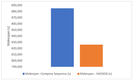
Figure 2.
Makespan comparison of the industrial scheduling problem.
4.2. Random Benchmark Problems
We performed simulation experiments with various parameter values to analyze the efficiency of this approach. The factor levels of the experimental design are outlined in Table 3. The problem description is presented in Table 4. The numbers of jobs are 20, 50, and 100. The number of stages is 5, 10, and 20. The number of machines in each stage is 2, 3, and 5. The real industrial scheduling problems might have a similar number of jobs, stages, and machines. The population size and the number of iterations are the two key parameters of the proposed HAOSOA. The small values of these two parameters would lead to poor diversity, whereas the too large values need a higher computational cost. To balance the diversity and computational cost, the population size is considered to be 100 and 200. The number of iterations is considered to be 200 and 500. Based on these values (3 × 3 × 3 × 1 × 2 × 2), 108 experiments were performed. The algorithm is run 20 times, and the average makespan value is considered. The algorithm’s efficacy was subsequently evaluated by juxtaposing it with previously examined algorithms. The efficacy of the proposed algorithm was assessed in comparison to alternative solutions utilizing the percentage deviation index (PDI). Equation (22) facilitated the determination of the PDI. It indicates the deviation of the makespan value obtained using different algorithms with respect to the optimal makespan value. The smaller PDI means the algorithm has a better solution quality on the test problem.
Table 3.
Factor levels for the design of experiments.
Table 4.
Problem description.
is value of the attained objective function.
is the optimal value of objective function.
The results of the HAOSOA were compared with the adaptive shuffled frog-leaping algorithm (ASFLA) [19], GA [6], Hybrid GA (HGA) [10], improved GA (IMGA) [6], and iterated greedy algorithm (IGA) [20]. The results are presented in Table 5. The table shows that the HAOSOA achieves about 1–4% better results over other methods. Though this value seems to be smaller, it is still significant. Geetha et al. [45] proved that the reduction in makespan would minimize the total energy cost and hence the environmental impact. Hence, even if the proposed algorithm reduces the makespan by 1–4%, it would reduce the total energy cost as well as the environmental impacts such as global warming, climate change, and greenhouse effect.
Table 5.
Percentage deviation index comparison of different algorithms.
4.2.1. Effectiveness Analysis
To evaluate the effectiveness and generalizability of the proposed HAOSOA, the HAOSOA was tested on a diverse set of random benchmark instances with varying characteristics:
- Small-scale instances (jobs × stages × machines: 20 × 5 × 2)
- Medium-scale instances (jobs × stages × machines: 50 × 10 × 3)
- Large-scale instances (jobs × stages × machines: 100 × 20 × 5)
The PDI values of HAOSOA and other algorithms shown in Table 5 indicated that the AOSOA consistently achieved lower PDI values, demonstrating its effectiveness across different HFS configurations.
4.2.2. Sensitivity Analysis
The sensitivity analysis was conducted to understand how the performance of HAOSOA is affected by its key parameters. The population number and the iteration number are the two key parameters of HAOSOA. The population size was 100 and 200. The number of iterations was 200 and 500. The PDI values indicate that HAOSOA exhibits stable performance over a reasonable range of parameter values, confirming its robustness.
4.2.3. Statistical Analysis of Results
We employed statistical analysis to evaluate the outcomes and assess the efficacy of diverse strategies.
4.2.4. Friedman Test
It has been asserted by numerous individuals that the Friedman test is used to examine the interaction between two or more independent variables. In the event of the null hypothesis being accepted, all the tactics are essentially the same. Given the lack of adherence to this hypothesis, it is conceivable that the cases under scrutiny demonstrated varying performance levels. The Friedman test evaluates algorithms based on their suitability for each data set and it is asserted that Rank 1 is the most efficient technique, followed by Rank 2 and subsequent ranks [47]. Table 6 displays the Friedman test results. The test indicates that HAOSOA is the most efficient algorithm, with a rating of 1.00. The p-value shows significant differences among the algorithms.
Table 6.
Friedman test results.
4.2.5. Wilcoxon Signed Rank Test
Two instances are evaluated to belong to distinct categories utilizing the Wilcoxon signed-rank test. It has been hypothesized by numerous researchers that this non-parametric measure is equivalent to the paired t-test. The objective of this two-sample test is to identify statistically significantly different means of 2 sample means or 2 outputs of an algorithm [47]. Table 7 encapsulates the test results. The HAOSOA algorithm outperforms by improving the solution quality against the other algorithms for each problem instance.
Table 7.
Wilcoxon test results.
4.3. Benchmark Problems
To validate the performance of the proposed algorithm, the benchmark problems proposed by Carlier and Neron [48] are considered in this work. Ten and fifteen jobs are considered in the benchmark problems. The number of stages is 5 and 10. The makespan results of the proposed algorithm are compared with the PSO [49], quantum-inspired immune algorithm (QIA) [50], ant colony optimization (ACO) algorithm [51], artificial immune system (AIS) algorithm [52], and AOSOA. Among the above algorithms, the PSO [49], AIS [52], AOSOA, and the HAOSOA can solve all 77 problems. The makespan comparison of different algorithms on benchmark problems is presented in Table 8. Based on the pairwise comparison, HAOSOA finds the exact solutions in 65 cases. However, in 12 problems, HAOSOA found slightly worse solution values than the lower bound (LB). Comparing HAOSOA against PSO, in 68 problems, solutions are the same, whereas in 9 problems, HAOSOA finds better solutions. QIA [50] is only able to solve 41 case problems. 29 of them have the same makespan value as HAOSOA, and in 12 problems, HAOSOA can find a better makespan. HAOSOA performs equal to or better than AOSOA, and in some cases, the results of HAOSOA exactly match the lower bound where AOSOA slightly deviates. PSO, AIS, and AOSOA provide similar results for most of the problems. Similar to QIA [50], ACO [51] can only solve 63 case problems, and 40 of them have a similar makespan with HAOSOA. In 18 problems, HAOSOA produces better makespan, but in 5 case problems, ACO [51] has better makespan values. Finally, in 65 cases, there is a tie between the AIS algorithm [52] and HAOSOA, whereas in 12 cases, HAOSOA finds a better makespan than the AIS. The results demonstrate that the HAOSOA is a highly competitive and stable method for solving the hybrid flow shop scheduling problems. It performs on par or better than other algorithms. The consistent performance of the HAOSOA makes it a strong candidate for real-world scheduling applications.
Table 8.
Makespan comparison of different algorithms on benchmark problems.
5. Conclusions
This paper examines the scheduling difficulties of a mixed-flow plant and the potential to minimize its makespan. A unique metaheuristic termed atomic orbital search optimization has been created to tackle this problem. Positive heuristics were employed to enhance response quality. The performance of the proposed HAOSOA was tested with the industrial scheduling problem of an electrical panel board manufacturing industry. Results indicated that the HAOSOA reduced the makespan by 6%. Randomly selected problems were utilized to assess the program’s performance. The efficacy of the recommended method was assessed against other previously documented strategies. The statistical study revealed the proposed algorithm’s effectiveness. The proposed technique has been demonstrated to be statistically efficient. The performance of the proposed algorithm was also verified using the benchmark problems existing in the literature. The results proved that the HAOSOA is superior to many other algorithms. Although this study is based on several assumptions, it shows potential for future advancement in addressing the HFS timing challenge. Eliminating these assumptions may enhance the proposed technique. The potential to combine the atomic orbital search optimization algorithm with other heuristics or metaheuristics to achieve better results is another promising aspect of this study. Furthermore, the proposed technique may be utilized to handle scheduling problems with sustainable objective functions, offering hope for significant improvements in this area of study. In this study, only the HFS environment is investigated with the help of HAOSOA. Two different benchmark problem sets are used to evaluate the proposed algorithm’s performance against other metaheuristics. Based on the first test benchmark, HAOSOA performs better in each of the 108 test instances against ASFLA, GA, HGA, IMGA, and IGA. In the second problem set, the proposed algorithm was able to solve all 77 cases and found the best values in 65 of them.
This study is limited only to the HFS environment, but to understand the nature of the HAOSOA, different scheduling environments can be analyzed in further studies. Also, different test problems can be used to compare the algorithm against other metaheuristics.
Author Contributions
Conceptualization, G.A. and M.K.M.; methodology, P.M.; software, M.K.M.; validation, M.K.M. and G.A.; formal analysis, Ö.T.; data curation, Ö.T.; writing—original draft preparation, G.A.; writing—review and editing, M.K.M.; supervision, M.K.M.; project administration, Ö.T. All authors have read and agreed to the published version of the manuscript.
Funding
This research received no external funding.
Data Availability Statement
The original contributions presented in this study are included in the article. Further inquiries can be directed to the corresponding author.
Conflicts of Interest
The authors declare no conflicts of interest.
References
- Pinedo, M.L. Scheduling: Theory, Algorithms, and Systems; Springer: Cham, Switzerland, 2016. [Google Scholar]
- Gholami, H.; Sun, H. Toward automated algorithm configuration for distributed hybrid flow shop scheduling with multiprocessor tasks. Knowl. Based Syst. 2023, 264, 110309. [Google Scholar] [CrossRef]
- Lei, D.; Su, B. A multi-class teaching–learning-based optimization for multi-objective distributed hybrid flow shop scheduling. Knowl. Based Syst. 2023, 263, 110252. [Google Scholar] [CrossRef]
- Allaoui, H.; Artiba, A. Scheduling two-stage hybrid flow shop with availability constraints. Comput. Oper. Res. 2006, 33, 1399–1419. [Google Scholar] [CrossRef]
- Jabbarizadeh, F.; Zandieh, M.; Talebi, D. Hybrid flexible flowshops with sequence-dependent setup times and machine availability constraints. Comput. Ind. Eng. 2009, 57, 949–957. [Google Scholar] [CrossRef]
- Luo, H.; Huang, G.Q.; Zhang, Y.; Dai, Q.; Chen, X. Two-stage hybrid batching flowshop scheduling with blocking and machine availability constraints using genetic algorithm. Robot. Comput. Integr. Manuf. 2009, 25, 962–971. [Google Scholar] [CrossRef]
- Zandieh, M.; Gholami, M. An immune algorithm for scheduling a hybrid flow shop with sequence-dependent setup times and machines with random breakdowns. Int. J. Prod. Res. 2009, 47, 6999–7027. [Google Scholar] [CrossRef]
- Behnamian, J.; Ghomi, S.F. Hybrid flowshop scheduling with machine and resource-dependent processing times. Appl. Math. Model. 2011, 35, 1107–1123. [Google Scholar] [CrossRef]
- Choi, S.H.; Wang, K. Flexible flow shop scheduling with stochastic processing times: A decomposition-based approach. Comput. Ind. Eng. 2012, 63, 362–373. [Google Scholar] [CrossRef][Green Version]
- Kianfar, K.; Ghomi, S.F.; Jadid, A.O. Study of stochastic sequence-dependent flexible flow shop via developing a dispatching rule and a hybrid GA. Eng. Appl. Artif. Intell. 2012, 25, 494–506. [Google Scholar] [CrossRef]
- Mirabi, M.; Ghomi, S.F.; Jolai, F. A two-stage hybrid flowshop scheduling problem in machine breakdown condition. J. Intell. Manuf. 2013, 24, 193–199. [Google Scholar] [CrossRef]
- Wang, K.; Choi, S.H.; Qin, H.; Huang, Y. A cluster-based scheduling model using SPT and SA for dynamic hybrid flow shop problems. Int. J. Adv. Manuf. Technol. 2013, 67, 2243–2258. [Google Scholar] [CrossRef]
- Ebrahimi, M.; Ghomi, S.F.; Karimi, B. Hybrid flow shop scheduling with sequence dependent family setup time and uncertain due dates. Appl. Math. Model. 2014, 38, 2490–2504. [Google Scholar] [CrossRef]
- Wang, K.; Choi, S.H. A holonic approach to flexible flow shop scheduling under stochastic processing times. Comput. Oper. Res. 2014, 43, 157–168. [Google Scholar] [CrossRef]
- Wang, Z.; Deng, Q.; Zhang, L.; Li, H.; Li, F. Joint optimization of integrated mixed maintenance and distributed two-stage hybrid flow-shop production for multi-site maintenance requirements. Expert Syst. Appl. 2023, 215, 119422. [Google Scholar] [CrossRef]
- Liu, Y.; Shen, W.; Zhang, C.; Sun, X. Agent-based simulation and optimization of hybrid flow shop considering multi-skilled workers and fatigue factors. Robot. Comput. Integr. Manuf. 2023, 80, 102478. [Google Scholar] [CrossRef]
- Maciel, I.S.F.; Prata, B.A.; Nagano, M.S.; Abreu, L.R. A hybrid genetic algorithm for the hybrid flow shop scheduling problem with machine blocking and sequence-dependent setup times. J. Proj. Manag. 2022, 7, 201–206. [Google Scholar] [CrossRef]
- Fu, Y.; Zhou, M.; Guo, X.; Qi, L. Scheduling Dual-Objective Stochastic Hybrid Flow Shop with Deteriorating Jobs via Bi-Population Evolutionary Algorithm. IEEE Trans. Syst. Man Cybern. Syst. 2020, 50, 5037–5048. [Google Scholar] [CrossRef]
- Deming, L.; Tao, D. An adaptive shuffled frog-leaping algorithm for parallel batch processing machines scheduling with machine eligibility in fabric dyeing process. Int. J. Prod. Res. 2024, 62, 7704–7721. [Google Scholar] [CrossRef]
- Yu, F.; Lu, C.; Zhou, J.; Yin, L. Mathematical model and knowledge-based iterated greedy algorithm for distributed assembly hybrid flow shop scheduling problem with dual-resource constraints. Expert Syst. Appl. 2024, 239, 122434. [Google Scholar] [CrossRef]
- Zhang, W.; Li, C.; Gen, M.; Yang, W.; Zhang, G. A multiobjective memetic algorithm with particle swarm optimization and Q-learning-based local search for energy-efficient distributed heterogeneous hybrid flow-shop scheduling problem. Expert Syst. Appl. 2024, 237, 121570. [Google Scholar] [CrossRef]
- Geetha, M.; Chandra Guru Sekar, R.; Marichelvam, M.K.; Tosun, Ö. A Sequential Hybrid Optimization Algorithm (SHOA) to Solve the Hybrid Flow Shop Scheduling Problems to Minimize Carbon Footprint. Processes 2024, 12, 143. [Google Scholar] [CrossRef]
- Abd Elaziz, M.; Ouadfel, S.; Abd El-Latif, A.A.; Ali Ibrahim, R. Feature selection based on modified bio-inspired atomic orbital search using arithmetic optimization and opposite-based learning. Cogn. Comput. 2022, 14, 2274–2295. [Google Scholar] [CrossRef]
- Ali, F.; Sarwar, A.; Bakhsh, F.I.; Ahmad, S.; Shah, A.A.; Ahmed, H. Parameter extraction of photovoltaic models using atomic orbital search algorithm on a decent basis for novel accurate RMSE calculation. Energy Convers. Manag. 2023, 277, 116613. [Google Scholar] [CrossRef]
- Azizi, M. Atomic orbital search: A novel metaheuristic algorithm. Appl. Math. Model. 2021, 93, 657–683. [Google Scholar] [CrossRef]
- Azizi, M.; Mohamed, A.W.; Shishehgarkhaneh, M.B. Optimum design of truss structures with atomic orbital search considering discrete design variables. In Handbook of Nature-Inspired Optimization Algorithms: The State of the Art: Volume II: Solving Constrained Single Objective Real-Parameter Optimization Problems; Springer International Publishing: Cham, Switzerland, 2022; pp. 189–214. [Google Scholar]
- Azizi, M.; Talatahari, S.; Giaralis, A. Optimization of engineering design problems using atomic orbital search algorithm. IEEE Access 2021, 9, 102497–102519. [Google Scholar] [CrossRef]
- Azizi, M.; Talatahari, S.; Khodadadi, N.; Sareh, P. Multiobjective atomic orbital search (MOAOS) for global and engineering design optimization. IEEE Access 2022, 10, 67727–67746. [Google Scholar] [CrossRef]
- Baghalzadeh Shishehgarkhaneh, M.; Fardmoradinia, S.; Keivani, A.; Azizi, M. BIM-based resource trade-off in dam project scheduling using Atomic Orbital Search (AOS) algorithm. AUT J. Civ. Eng. 2023, 6, 469–492. [Google Scholar]
- Elaziz, M.A.; Abualigah, L.; Yousri, D.; Oliva, D.; Al-Qaness, M.A.; Nadimi-Shahraki, M.H.; Ewees, A.A.; Lu, S.; Ali Ibrahim, R. Boosting atomic orbit search using dynamic-based learning for feature selection. Mathematics 2021, 9, 2786. [Google Scholar] [CrossRef]
- Hussain, M.T.; Tariq, M.; Sarwar, A.; Urooj, S.; BaQais, A.; Hossain, M.A. Atomic orbital search algorithm for efficient maximum power point tracking in partially shaded solar PV systems. Processes 2023, 11, 2776. [Google Scholar] [CrossRef]
- Karakaş, M.F.; Latifoğlu, F. Metaheuristic FIR filter design with multi-objective atomic orbital search algorithm. Avrupa Bilim Ve Teknol. Derg. 2022, 39, 13–16. [Google Scholar]
- Ke, H.; Bi, J.; Wang, Y.; Zhang, Y. Driving range estimation for electric bus based on atomic orbital search and back propagation neural network. IET Intell. Transp. Syst. 2024, 18, 2884–2895. [Google Scholar] [CrossRef]
- Kiruthiga, B.; Karthick, R.; Manju, I.; Kondreddi, K. Optimizing harmonic mitigation for smooth integration of renewable energy: A novel approach using atomic orbital search and feedback artificial tree control. Prot. Control. Mod. Power Syst. 2024, 9, 160–176. [Google Scholar] [CrossRef]
- Kumar, R.; Bothara, Y.; Ezhilarasi, D.; Mohanavelu, K. Atomic Orbital Search Optimization Based Fractional Order PID Controller for 4 DoF Lower Limb Exoskeleton. In Proceedings of the 2023 International Conference on Power, Instrumentation, Control and Computing (PICC), Thrissur, India, 19–21 April 2023; pp. 1–6. [Google Scholar]
- Liu, G.; Zhao, T.; Yan, H.; Wu, H.; Wang, F. Evaluation of urban green building design schemes to achieve sustainability based on the projection pursuit model optimized by the atomic orbital search. Sustainability 2022, 14, 11007. [Google Scholar] [CrossRef]
- Mahdi Mudassir, S.M.; Salma, U. A hybrid technique for optimal sizing and performance analysis of hybrid renewable energy sources. Energy Environ. 2023, 36, 1617–1647. [Google Scholar] [CrossRef]
- Manita, G.; Chhabra, A.; Korbaa, O. Efficient e-mail spam filtering approach combining Logistic Regression model and Orthogonal Atomic Orbital Search algorithm. Appl. Soft Comput. 2023, 144, 110478. [Google Scholar] [CrossRef]
- Ozkaya, B. Optimal Parameter Estimation of PEMFC Model Using an Improved Atomic Orbital Search Algorithm. Appl. Model. Simul. 2024, 8, 283–300. [Google Scholar]
- Revanesh, M.; Rudra, B.; Guddeti, R.M.R. An Optimized Question Classification Framework Using Dual-Channel Capsule Generative Adversarial Network and Atomic Orbital Search Algorithm. IEEE Access 2023, 11, 75736–75747. [Google Scholar] [CrossRef]
- Rohit, P.; Datta, A.; Satyanarayana, M. Design of High Gain Metasurface Antennas using Hybrid Atomic Orbital Search and Human Mental Search Algorithm for IoT Application. In Proceedings of the 2023 10th International Conference on Signal Processing and Integrated Networks (SPIN), Noida, India, 23–24 March 2023; pp. 20–24. [Google Scholar]
- Saravanan, R.; Godwin Ponsam, J.; Sathiya, V.; Saranya, G. Air pollution monitoring approach using atomic orbital search algorithm with deep learning driven. Glob. NEST J. 2024, 26, 1–9. [Google Scholar]
- Zafar, M.H.; Khan, N.M.; Khan, U.A. Short term hybrid PV/Wind power forecasting for smart grid application using feedforward neural network (FNN) trained by a novel atomic orbital search (AOS) optimization algorithm. In Proceedings of the 2021 International conference on frontiers of information technology (FIT), Islamabad, Pakistan, 13–14 December 2021; pp. 72–77. [Google Scholar]
- Bean, B.C. Genetic algorithms and random keys for sequencing and optimization. ORSA J. Comput. 1994, 6, 154–160. [Google Scholar] [CrossRef]
- Geetha, M.; Chandra Guru Sekar, R.; Marichelvam, M.K. A Hybrid Honey Badger Algorithm to Solve Energy-Efficient Hybrid Flow Shop Scheduling Problems. Processes 2025, 13, 174. [Google Scholar] [CrossRef]
- Nawaz, M.; Enscore, E.E., Jr.; Ham, I. A heuristic algorithm for the m-machine, n-job flow-shop sequencing problem. Omega 1983, 11, 91–95. [Google Scholar] [CrossRef]
- Tosun, Ö. Using artificial bee colony algorithm for permutation flow shop scheduling problem under makespan criterion. Int. J. Math. Model. Numer. Optim. 2014, 5, 191–209. [Google Scholar] [CrossRef]
- Carlier, J.; Neron, E. An exact method for solving the multi-processor flow-shop. RAIRO Oper. Res. Rech. Opérationnelle 2000, 34, 1–25. [Google Scholar] [CrossRef]
- Liao, C.J.; Tjandradjaja, E.; Chung, T.P. An approach using particle swarm optimization and bottleneck heuristic to solve hybrid flow shop scheduling problem. Appl. Soft Comput. 2012, 12, 1755–1764. [Google Scholar] [CrossRef]
- Niu, Q.; Zhou, T.; Ma, S. A quantum-inspired immune algorithm for hybrid flow shop with makespan criterion. J. Univers. Comput. Sci. 2009, 15, 765–785. [Google Scholar]
- Alaykýran, K.; Engin, O.; Döyen, A. Using ant colony optimization to solve hybrid flow shop scheduling problems. Int. J. Adv. Manuf. Technol. 2007, 35, 541–550. [Google Scholar] [CrossRef]
- Engin, O.; Döyen, A. A new approach to solve hybrid flow shop scheduling problems by artificial immune system. Future Gener. Comput. Syst. 2004, 20, 1083–1095. [Google Scholar] [CrossRef]
Disclaimer/Publisher’s Note: The statements, opinions and data contained in all publications are solely those of the individual author(s) and contributor(s) and not of MDPI and/or the editor(s). MDPI and/or the editor(s) disclaim responsibility for any injury to people or property resulting from any ideas, methods, instructions or products referred to in the content. |
© 2025 by the authors. Licensee MDPI, Basel, Switzerland. This article is an open access article distributed under the terms and conditions of the Creative Commons Attribution (CC BY) license (https://creativecommons.org/licenses/by/4.0/).