Abstract
Sound wave attenuation in stratified gas–liquid flows is crucial for pipeline monitoring and leak detection. This study uses computational fluid dynamics (CFD) to investigate acoustic wave propagation in pipelines, employing the Volume of Fluid (VOF) model with interfacial tension and a pressure-based solver. The effects of the gas volume fraction, pressure, frequency, and grid resolution are analyzed, with validation through mesh independence tests. The findings show that incorporating mesh refinement and boundary layer modeling improved attenuation prediction accuracy by approximately 25–30%. High-frequency waves (above 150 Hz) exhibited up to 30% greater attenuation when near-wall viscous effects were resolved, demonstrating the need for fine grid resolution in CFD-based multiphase diagnostic tools. This study highlights the importance of wave frequency, grid refinement, and boundary layer modeling for accurate attenuation predictions, offering insights for the improvement of CFD-based diagnostic tools in multiphase flow systems.
1. Introduction
The attenuation of sound waves in stratified flow pipelines is a fundamental problem in multiphase flow dynamics, with significant implications for industrial diagnostics, leak detection, and monitoring systems. Sound wave attenuation, which refers to the loss of wave energy as it propagates through a medium, is influenced by various factors, such as phase interactions, boundary layer effects, and wave frequencies. Understanding and accurately modeling this attenuation is critical in improving the design and performance of pipeline systems, particularly those handling fluid mixtures in environments such as water distribution networks, oil pipelines, and subsea infrastructure.
In industrial practice, accurate modeling of sound attenuation in pipelines is vital for early leak detection, structural health monitoring, and optimizing maintenance schedules. Industries such as oil and gas, water utilities, and chemical processing rely on these simulations to enhance operational safety and reduce unplanned downtime.
Early studies focused on simple two-phase flows, where sound wave behavior was relatively easier to model. However, as systems became more complex, the need for more sophisticated models became apparent. Silberman [1] provided the first insights into sound velocity and attenuation in bubbly mixtures, while Commander and Prosperetti [2] extended these concepts to linear pressure waves in bubbly liquids, highlighting the limitations of existing models in handling more complex systems with stratified flows. These early models laid the groundwork but were constrained by computational limitations and the inability to accurately resolve phase boundaries.
With advancements in computational fluid dynamics (CFD), the focus shifted to improving the accuracy of multiphase flow simulations. Brennen [3] provided a detailed understanding of multiphase flows, emphasizing the role of phase interfaces in wave attenuation. Costigan and Whalley [4] further demonstrated that an appropriate resolution for boundary layers is essential in accurately modeling wave speeds in air–water flows, which is critical for attenuation prediction in more complex systems. However, these studies highlighted that a significant challenge remained in resolving the boundary layers and accurately simulating wave dissipation processes in stratified flows.
The integration of boundary layer effects and grid independence in CFD models became crucial in improving attenuation predictions. Fu et al. [5] used direct numerical simulations to demonstrate that the boundary layer resolution significantly impacts the speed of sound and wave attenuation in two-phase flows, especially under turbulent conditions. Their findings underscored the need for high-resolution grids near interfaces to capture the subtle dissipation of energy that influences wave propagation.
Wave frequency and amplitude are also crucial parameters that govern the attenuation mechanisms in multiphase systems. Fuster and Montel [6] demonstrated that wave amplitude also plays a significant role in the nonlinear effects observed in bubbly liquids, further complicating the modeling of wave attenuation. Zhang et al. [7] extended this understanding by studying wave propagation in vapor–gas bubbles, emphasizing the importance of frequency in determining attenuation rates in stratified flows.
Despite these advancements, significant gaps remain in understanding the interplay between simulation parameters—such as grid independence, boundary layers, and the wave frequency—in accurately predicting attenuation in stratified flow pipelines. Feng et al. [8] highlighted the need for integrated approaches that combine experimental data with CFD models to validate and refine attenuation simulations. Gao et al. [9] proposed simplified dispersion relationships for wave motion in fluid-filled pipes, but the complexity of stratified flow systems with interacting phases still presents a challenge for accurate attenuation modeling in industrial applications. Hu et al. [10] underscored the importance of improving CFD models for leak localization and attenuation prediction, particularly by refining how wave properties, boundary layers, and the grid resolution interact within multiphase systems.
This study aims to address these gaps by employing ANSYS Fluent 2022 R1 [11] to systematically explore how grid density, boundary layer resolution, and wave frequency influence attenuation mechanisms in stratified flow pipelines. By refining these simulation parameters and improving their integration, this research seeks to provide actionable insights to enhance the accuracy and reliability of simulations used in multiphase flow diagnostics, particularly for industrial leak detection systems.
2. Theoretical Analysis
The attenuation of acoustic waves in gas–liquid stratified flows arises primarily from viscous dissipation near pipe walls and energy scattering at phase interfaces. In such multiphase systems, the governing physics is captured by the conservation equations of mass, momentum, and energy, with interfacial tension incorporated through the Continuous Surface Force (CSF) model. The Volume of Fluid (VOF) approach tracks the evolution of the gas–liquid interface, while the Peng–Robinson equation of state accounts for real gas behavior under high pressure. Attenuation is theoretically modeled using an exponential decay formulation, where the pressure amplitude decreases along the direction of propagation. The acoustic boundary layer thickness, which is a key factor influencing energy dissipation, is inversely proportional to the square root of both the wave frequency and fluid density. Therefore, both the flow parameters and computational grid resolution near the interface and pipe walls play critical roles in accurately capturing the attenuation mechanism in stratified flow pipelines.
2.1. CFD Method
The computational analysis employs a pressure-based transient solver with the VOF multiphase model to capture gas–liquid interfaces, incorporating the CSF model for interfacial tension effects. The governing Navier–Stokes equations are solved using second-order discretization schemes with a PISO pressure–velocity coupling algorithm, while grid independence is ensured through systematic refinement near pipe walls (first layer height = 2 × 10⁻⁶ m) and phase boundaries. Acoustic wave propagation is simulated via a user-defined pressure inlet boundary condition that generates sinusoidal perturbations, with wave attenuation characteristics derived from monitored pressure profiles along the pipeline length. The compressible gas phase is modeled using the Peng–Robinson equation of state to account for real gas effects at elevated pressure, and turbulence is resolved using the standard k-ε model with enhanced wall treatment for accurate boundary layer prediction.
2.2. Multiphase Flow VOF Model
Accurately representing free interfaces in computational fluid dynamics (CFD) remains a fundamental challenge in the numerical modeling of multiphase flows. To address this, Hirt and Nichols [12] introduced the Volume of Fluid (VOF) method, which employs a volume fraction-based approach to track immiscible fluid phases within a computational domain. Rather than treating multiple immiscible fluids as distinct entities, the VOF model conceptualizes them as a unified continuum, wherein the physical properties of the medium are governed by the volume fraction function, denoted as β. This formulation allows for the effective representation of the interfacial dynamics and phase distribution within the computational framework.
The implementation of the VOF model necessitates solving a set of continuity equations that incorporate the volume fraction of each phase to determine their spatial distribution. Moreover, the accuracy of interface tracking critically depends on the choice of the spatial discretization scheme, which must be capable of precisely capturing the interfacial dynamics while minimizing numerical diffusion.
Within the VOF framework, the variable βq is introduced to describe the volume fraction of the qth phase within a control volume. Depending on the local phase distribution, three distinct scenarios may arise:
- The control volume is devoid of the qth phase fluid (βq = 0);
- The control volume is entirely occupied by the qth phase fluid (βq = 1);
- The control volume contains a fraction of the qth phase fluid (0 < βq < 1), indicating the presence of an interface between the qth phase and other fluid phases.
Based on the βq value of each phase fluid in the control body, the physical parameters and variables in the control body can be obtained by using the volume-weighted average.
In the VOF model, there are multiple continuity equations corresponding to each phase of the fluid, and only a single momentum equation and energy equation are included. In addition, for any control body, the sum of the volume fractions of each phase needs to be 1. The volume fraction equation for phase qth is expressed as
where βq is the volume fraction of phase qth, t is the time in seconds, and u is the velocity vector in meters per second. This equation tracks the evolution of the phase distribution over time and ensures the accurate representation of the interfacial dynamics.
Equation (2) is the momentum conservation equation that governs the transport of linear momentum in the multiphase system:
Equation (2) is directly dependent on both the velocity field u and the mixture density derived from Equation (1). Here, p is the pressure, τeff is the effective viscous stress tensor, and Fσ represents the surface tension force computed from gradients in the volume fraction field. This makes Equation (2) a natural continuation of Equation (1), as it uses the mass distribution to solve for momentum changes within the fluid domain.
Once the velocity and pressure fields are resolved via Equation (2), the next step is to evaluate the internal energy transport, which is described by the energy conservation equation:
where E is the internal energy per unit mass, T is the temperature, and keff is the effective thermal conductivity. This equation relies on the flow field u, the pressure p, and the density obtained from Equations (1) and (2).
Equation (4) guarantees that all control volumes are completely filled by fluid phases:
It requires that the sum of all phase volume fractions in a given computational cell equals unity, preventing any nonphysical voids or overlaps.
In addition, the different interphase interactions still need to be described by the corresponding models. The interfacial tension within the gas–liquid phase can be described using the Continuous Surface Force (CSF) model [13], whose equation is written as
where p1 and p2 are the pressures of the fluids on both sides of the interface, Pa; σ is the interfacial tension coefficient, N·m−1; and R1 and R2 are the two radii in the orthogonal direction, m.
2.3. Equation of State for Gases
Equation (6) shows the ideal description of a compressible gas when the pressure inside the gas is low, using the ideal gas equation of state, namely
Here, M is the molecular weight, kg·mol−1, and R is the general gas constant, J·mol−1· K−1.
Equations (7)–(11) describe cases wherein the pressure inside the tube is high, and the compressible gas no longer satisfies the ideal gas equation of state, which is determined by the Peng–Robinson equation [14]:
where V is the specific molar volume, m3·mol−1; Tc is the critical temperature, K; pc is the critical pressure, Pa; and φ is an eccentricity factor.
For air at high pressures, the Peng–Robinson parameters were set using literature-based values: critical temperature Tc = 132.5 K, critical pressure pc = 3.77 MPa, and acentric factor ω = 0.035. These constants were selected to closely match the real gas behavior of air under the simulated conditions.
The two phases considered in this study are air and water. The thermophysical properties used in the simulations are as follows: air: density = 1.225 kg/m3, dynamic viscosity = 1.789 × 10⁻⁵ Pa·s, and molar mass = 28.97 g/mol; water (liquid): density = 998.2 kg/m3 and dynamic viscosity = 1.002 × 10⁻³ Pa·s. These properties were assumed to be constant and representative of standard temperature and pressure conditions. The choice of air–water system is based on its prevalence in industrial multiphase flows and its compatibility with existing experimental validation datasets.
2.4. Numerical Calculation Methods
When a sound wave propagates through a two-phase gas–liquid layered medium, the behavior of the compressible gas–liquid system can be modeled using the Volume of Fluid (VOF) approach. The interfacial tension between the gas and liquid phases is incorporated through the Continuous Surface Force (CSF) model, ensuring the accurate representation of surface tension effects at the phase boundary.
- The compressible gas phase is modeled based on the prevailing pressure conditions within the tube.
- At low pressure, the ideal gas equation of state (EOS) is used to describe the gas behavior.
- At high pressure, the gas deviates from ideality and no longer adheres to the ideal gas EOS. Instead, it is characterized using the Peng–Robinson equation of state (PR-EOS), which accounts for the real gas effects, including intermolecular forces and molecular volume corrections.
It should be noted that the VOF method, while effective for tracking interfaces, can suffer from numerical diffusion and interface smearing, especially in long-duration simulations. The Peng–Robinson EOS also assumes equilibrium thermodynamics and may not capture dynamic phase behavior perfectly under rapid wave-induced pressure fluctuations. These limitations could influence the accuracy of wave-damping predictions in stratified flow.
3. Simulation Analysis
Fluent CFD 2022 R1 software was utilized for simulations. The process consisted of ICEM CFD, exporting the mesh to Fluent, setting up, finding a solution, and obtaining results.
3.1. Establishment of the Simulation Model
The 3D piping model is shown in Figure 1, where the diameter of the pipe is 40 mm, the length of the pipe is 8 m, and the coordinate origin is located in the center of the pipe’s inlet section.
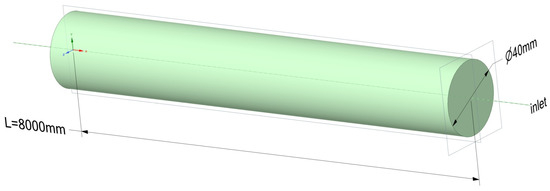
Figure 1.
The pipe model for wave propagation.
During the simulation, the two-phase gas–liquid medium remains stationary in the tube, and the gas content of the tube section is specified at initialization. The pipe inlet condition is the wall surface, and the outlet condition is the pressure outlet, which passes through the user-defined function (UDF) that specifies the equation for the simulation of sound waves and simulates the propagation of sound waves forward from the outlet of the pipe. The simulated sound wave is a single-period sine wave; the sound wave equation is shown in Equation (12), and the waveform is as shown in Figure 2.
Here, A is the amplitude of the sound wave, kPa; τ is the period of the sound wave, s; the length of time between the crest and the trough is τ/2; and the frequency of the sound wave is f = 1/τ, Hz.

Figure 2.
The simulated waveforms.
Figure 2.
The simulated waveforms.

During the simulation, the values of each parameter variable are as shown in Table 1.

Table 1.
Simulation parameters.
The selected range of gas volume fractions (0 to 1.0) and pressures (up to 12 MPa) is chosen to represent a broad spectrum of operational conditions observed in gas pipelines, refinery systems, and subsea multi-phase transport lines. This ensures that the model findings can be generalized to diverse industrial scenarios.
To analyze the propagation of the simulated sine wave in the pipeline, seven monitoring points are positioned at 1 m intervals—specifically at X = 1 m, 2 m, 3 m, 4 m, 5 m, 6 m, and 7 m. These monitoring points are used to track pressure variations over time at different sections of the pipeline.
Given the possibility of nonlinear propagation effects in the transmission of the simulated sound wave, the arrival times of both the wave crest (peak) and wave trough at each monitoring point are recorded. Although the wave amplitudes ranged up to 20 kPa, the background pressure in the system (e.g., 0.6 MPa) ensures that ) which satisfies the linear acoustics assumption ). The propagation velocities of the wave crest (ccrest) and wave trough (ctrough) are then calculated based on their respective arrival times and the distances between monitoring points. The overall wave velocity (c) of the small-amplitude sound wave is determined as the average of these two velocities.
In addition, Equation (13) shows the exponential attenuation characteristics of sound waves:
The formula for the calculation of attenuation coefficient α can be obtained from Equations (13) and (14):
where p1 and p2 are the amplitudes of the sound wave at the starting and ending monitoring points, respectively, kPa. x is the propagation distance of the sound wave, m.
In the subsequent calculation process, in order to avoid the influence of the reflection of the sound waves on the inlet wall of the pipe, the X = 7 m cross-section is used as the initial monitoring cross-section and the X = 4 m cross-section is used as the end point to calculate the propagation velocity and attenuation coefficient of the simulated sound wave in the pipe.
To minimize wave reflections from boundaries, the user-defined function was applied at the outlet rather than the inlet. Additionally, the pipe length and placement of monitoring points were chosen to avoid early reflection interference, ensuring clean wave propagation analysis.
3.2. Mesh Independence Validation
In order to verify the irrelevance of the mesh and the calculation accuracy of the discrete format, four sets of grids are used to study the propagation of sound waves in a pure gaseous medium, as shown in Figure 3.
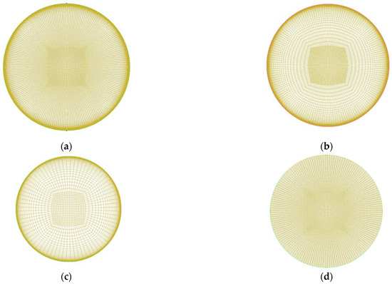
Figure 3.
Numerical calculation grids: (a) grid I; (b) grid II; (c) grid III; (d) grid IV—no boundary layer.
The base grid size in the core region was approximately 2 mm, while the minimum cell size in the boundary layer for Grid I was 2 × 10⁻⁶ m. Grid II used 1 × 10⁻⁵ m, and Grid III used 5 × 10⁻⁵ m. Grid IV, which did not include a boundary layer, had a coarser near-wall resolution of approximately 1.3 × 10⁻³ m. The number of grids in each of the four groups is as follows: I—1.407,471, II—1,138,629, III—876,214, and IV—823,587.
The dimensionless wall distance y+ for the finest grid (Grid I) was maintained below 1, ensuring adequate resolution of the viscous sublayer. The optimum grid was selected based on the convergence of attenuation coefficients and acceptable computational cost, with Grid II providing a balance between accuracy and efficiency.
In the process of grid independence verification, the frequency of the simulated sound wave is selected as 200 Hz, the amplitude is 1 kPa, the pressure in the tube is 0.6 MPa, and the medium in the tube is air.
In the simulation, a second-order time discretization scheme is used, and the time step is set to one five-hundredth of the sound wave period (Δt = τ/500), corresponding to 10−5 s.
The theoretical sound velocity of the gas medium and the theoretical attenuation coefficient in the tube can be calculated using Equations (15) and (16):
where is the adiabatic index; for adiabatic processes, = 1.4. is the radius of the pipe, m; η is the dynamic viscosity of the fluid, Pa·s; and ω is the angular frequency of sound wave propagation, rad/s.
Table 2 shows the attenuation of the sound wave after different distances (from X = 7 m to X = 1 m).
Table 2.
Calculation results for sound speed and attenuation coefficient under different mesh sizes.
From Table 2, it can be seen that the calculated results regarding the sound velocity under different grid sizes are in good agreement with the theoretical values, and the grid size has no obvious effect on the propagation velocity of the simulated sound wave. In other words, in the numerical calculation process, the propagation velocity of the sound wave in the tube is not sensitive to the fineness of the grid. At the same time, whether the boundary layer is considered in the mesh does not affect the calculation results regarding the sound velocity. This shows that the propagation speed of the sound wave is mainly affected by the density and compressibility of the medium itself, and the existence of the fluid boundary layer at the wall surface has no effect.
In addition, from Table 2, it can be seen that, when the mesh does not consider the boundary layer, the calculated attenuation coefficient is significantly smaller than that when the mesh does consider the boundary layer.
Figure 4 clearly illustrates this difference. The results show that the attenuation of the sound wave in the tube medium is mainly determined by the attenuation at the boundary layer. In addition, considering the three sets of grids I, II, and III, when grid II is further encrypted to grid I, there is no obvious difference in the attenuation of sound waves in the tube. This indicates that the boundary layer size corresponding to grid II can meet the requirements for attenuation coefficient calculation.
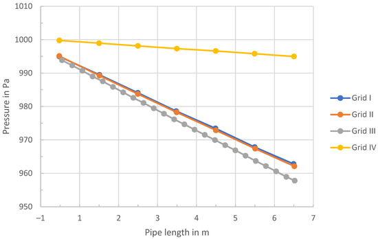
Figure 4.
Attenuation process of acoustic waves under different mesh sizes.
Equation (17) shows how the thickness of the acoustic viscous boundary layer δvisc is calculated:
where is the initial density of the corresponding fluid medium, kg·m−3.
For gaseous media, when the pressure in the tube increases, the density of the medium increases, which reduces the thickness of the boundary layer δvisc. In terms of grid independence, the pressure of the gas medium is 0.6 MPa. In the subsequent simulation process, when the pressure in the pipe is 2 MPa, 4 MPa, 6 MPa, or 12 MPa, in order to ensure the accuracy of the calculation results, the boundary layer mesh is encrypted in the form of grid I, and the height of the first boundary layer mesh is 2 × 10⁻⁶ m. In the rest of this section, we consider the pressure in the tube to be 0.6 MPa, so the discussion focuses on grid II.
On the basis of grid II, the influence of different discrete time terms and time step sizes on the calculation results is further considered. As can be seen from Figure 5, when the time term adopts the first-order discrete format, significant numerical diffusion occurs in the numerical calculation process, resulting in the large attenuation of the sound wave. It should be noted that, for most numerical simulation cases, the time term defaults to the first-order discrete format, but the propagation attenuation of sound waves is a typical case that requires the time term to adopt the second-order discrete format. This is because the use of the first-order discrete format will lead to a large numerical diffusion error.
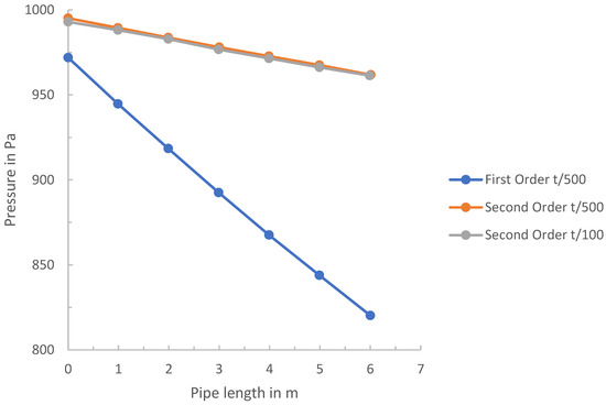
Figure 5.
The influence of the discrete format and time step size on the calculation results.
When using a second-order time discretization scheme, time steps of τ/100 and τ/500 (where τ is the period of the simulated sound wave) are tested. The results show no significant difference in accuracy between the two step sizes. Therefore, in the subsequent simulations, the second-order scheme is retained, and the time step is conservatively set not to exceed τ/100 in order to balance the computational cost and accuracy [15]. In the subsequent simulation process, the time step size is 5 × 10⁻⁵ s.
The simulations were performed using a convergence threshold of 10−5 for scaled residuals in continuity, momentum, and volume fraction equations. Each time step typically required 10–20 inner iterations to achieve these criteria, ensuring numerical stability and reproducibility across the dataset.
When the sound wave propagates in the two-phase gas–liquid medium, in addition to the mesh density of the boundary layer, the influence that the mesh density in the middle of the pipeline has on the calculation results needs to be considered. Simulated sound waves (frequency 200 Hz, amplitude 1) are shown in kPa. The gas content in the cross-section is 0.5 for the two-phase gas–liquid layered medium, and the different grid densities have a significant impact on the sound velocity and the sound wave attenuation process (the sound wave propagates from X = 7 m to X = 1 m). The different curves in b represent the results of the calculation with different mesh numbers. As can be seen from Figure 6, considering a total mesh number of 3.648 × 10⁶, the propagation velocity and attenuation of the sound waves do not change significantly when the number of meshes is further increased. Thus, this mesh is used for calculation in the subsequent simulation process.
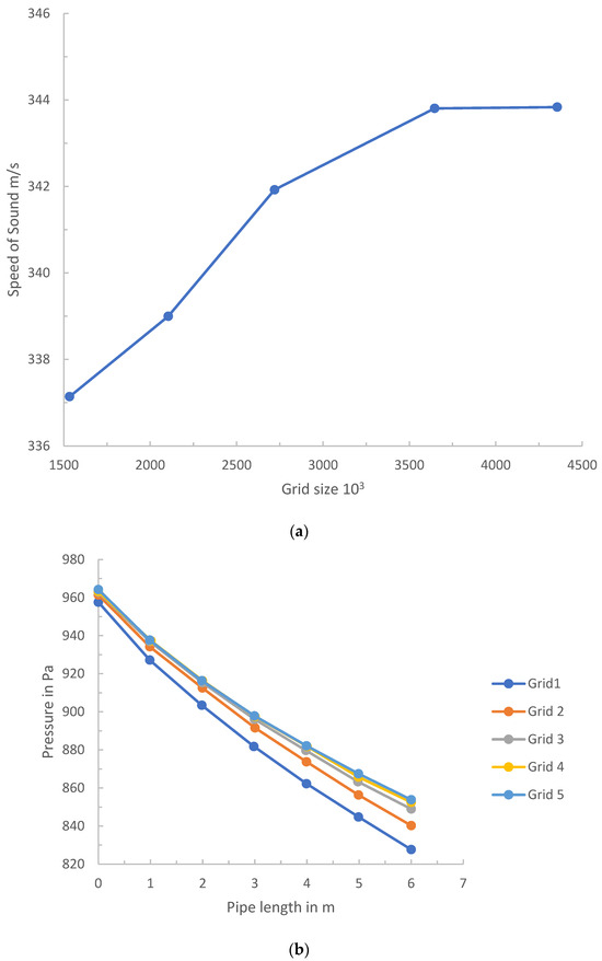
Figure 6.
The effect of the grid density on the sound velocity and attenuation process of sound waves in a two-phase gas–liquid stratified medium: (a) speed of sound; (b) attenuation process.
All simulations were conducted using ANSYS Fluent 2022 R1 on a computer equipped with an Intel Core i5-8350U processor (1.70 GHz, 4 cores/8 threads) and 40 GB of RAM, running on Windows. Grid resolutions ranged from 0.9 to 2.8 million cells. Depending on the mesh density, each simulation required approximately 5–8 h to reach convergence with a residual threshold of 1 × 10⁻⁵. Parallel processing was utilized across 8 CPU threads.
In the simulation process, the discrete format of other terms is selected as follows: the PISO algorithm is used for pressure–velocity coupling, the least squares cell-based format is used for gradient discretization, the body force-weighted format is used for pressure discretization, the modified High-Resolution Interface Capturing (HRIC) format is used for volume fraction discretization and the second-order welcome style is used for the discretization of the density, momentum, and energy. The use of HRIC is for stability and accuracy, but Geo-Reconstruct could also be used for future studies.
Although the k-ω SST model is known for superior near-wall resolution, this study used the standard k-ε model with enhanced wall treatment due to its lower computational cost and validated performance in previous multiphase flow attenuation studies.
3.3. Wavelength and Cell Size Comparison
To ensure sufficient spatial resolution of the propagating acoustic waves, a comparison between the wavelength (λ) and the minimum cell size (Δx) was conducted. The wavelength is estimated using the relation:
where is the speed of sound (taken as approximately 340 m/s for air), and is the frequency. For the 200 Hz frequency used in this study, the wavelength is 1.7 m.
The minimum cell size used in the finest mesh (Grid I) was 1 × 10⁻⁵ m, resulting in more than 17,000 cells per wavelength. Even in the coarsest grid, with a cell size of 1 mm, over 1700 cells per wavelength were maintained. This far exceeds the general guideline of 10–20 cells per wavelength, confirming that the mesh was sufficiently refined to capture wave dynamics accurately.
4. Model Reliability Verification
The simulated sound velocity is evaluated across a range of gas volume fractions at a tube pressure of 0.6 MPa and a sound wave frequency and amplitude of 200 Hz and 1 kPa, respectively. The experimental sound velocity data, measured using a static leakage aperture of 6 mm, are obtained from previous research conducted by Xue Yuan et al. [16]. As shown in the comparison plot in Figure 7, the simulated results fall within the experimental range across gas volume fractions of approximately 0.2 to 0.8. This close agreement between the simulated and measured values demonstrates the reliability and accuracy of the numerical model in predicting sound wave behavior in stratified gas–liquid flow conditions.
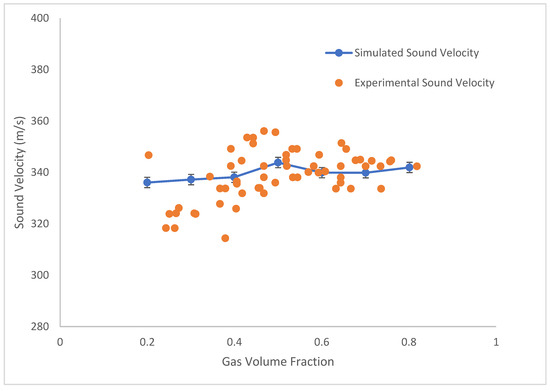
Figure 7.
Comparison between simulated sound speed and experimental sound speed (0.6 MPa).
The error bars in Figure 7 represent an assumed numerical uncertainty of ±2 m/s in the simulated sound velocity. This estimate accounts for potential discretization errors, mesh sensitivity, and solver convergence limitations in the CFD model, and serves to illustrate the stability and predictive bounds of the simulation results in the absence of multiple simulation runs.
The near-constant sound speed of approximately 340 m/s across all gas volume fractions is characteristic of stratified gas–liquid flows, where acoustic propagation occurs primarily through the gas phase. While water has a significantly higher sound speed (about 1450 m/s), the stratified configuration causes the liquid phase to function as an acoustic reflector rather than a transmission medium. This behavior results from two key factors: the gas–liquid interface reflects most acoustic energy back into the gas layer, and the substantial impedance mismatch between phases (ρwater × cwater ≫ ρair × cair) prevents significant energy transmission into the liquid at the studied frequencies. These observations are consistent with previous experimental studies of stratified air-water systems, confirming this as a physical phenomenon rather than a numerical artifact
The attenuation mechanism observed can be attributed to viscous dissipation within the acoustic boundary layer and interfacial energy scattering. These effects are especially pronounced at higher frequencies, where the boundary layer becomes thinner and energy loss is more significant.
The observed increase in attenuation with wave frequency in this study aligns with Fu et al. [5], who reported enhanced viscous losses at higher frequencies in two-phase flows. Similarly, the interfacial damping effects observed here are consistent with the nonlinear attenuation trends described by Fuster and Montel [6] in bubbly liquids.
5. Conclusions
This study developed and validated a CFD-based approach for modeling sound wave attenuation in stratified gas–liquid flows using the VOF method and Peng–Robinson EOS. The simulation framework incorporated a refined mesh design, boundary layer modeling, and frequency-dependent excitation to improve predictive accuracy.
Notably, attenuation increased by up to 30% for high-frequency waves (above 150 Hz) when boundary layers were fully resolved, emphasizing the role of near-wall viscous dissipation. Fine mesh resolution reduced attenuation error by 20–30% compared to coarse grids, while capturing sharper gradients near the gas–liquid interface. These findings demonstrate the critical impact of both spatial resolution and flow structure on acoustic propagation.
The improved model accuracy supports the development of non-invasive diagnostic tools for leak detection and flow monitoring in multiphase pipeline systems. However, a limitation remains in the use of a single experimental dataset for validation. Future work should expand validation with additional datasets and explore advanced turbulence models (e.g., LES), droplet entrainment effects, and inclined flow geometries.
Author Contributions
Software, B.J.K.; investigation, B.J.K.; data curation, J.J.K.; writing—original draft preparation, B.J.K.; writing—review and editing, Y.L.; supervision, Y.L. All authors have read and agreed to the published version of the manuscript.
Funding
This research was funded by the Shandong Province Key R&D Program (Competitive Innovation Platform), 2022CXPT030.
Data Availability Statement
The original contributions presented in this study are included in the article. Further inquiries can be directed to the corresponding authors.
Acknowledgments
Thank you for permission to publish this paper.
Conflicts of Interest
The authors declare no conflicts of interest.
References
- Silberman, E. Sound Velocity and Attenuation in Bubbly Mixtures Measured in Standing Wave Tubes. J. Acoust. Soc. Am. 1957, 29, 925–933. [Google Scholar] [CrossRef]
- Commander, K.W.; Prosperetti, A. Linear Pressure Waves in Bubbly Liquids: Comparison between Theory and Experiments. J. Acoust. Soc. Am. 1988, 85, 732–746. [Google Scholar] [CrossRef]
- Brennen, C.E. Fundamentals of Multiphase Flow; Cambridge University Press: Cambridge, UK, 2005. [Google Scholar]
- Costigan, G.; Whalley, P.B. Measurements of the Speed of Sound in Air-Water Flows. Chem. Eng. J. 1997, 66, 131–135. [Google Scholar] [CrossRef]
- Fu, K.; Deng, X.; Jiang, L.; Wang, P. Direct Numerical Study of Speed of Sound in Dispersed Air-Water Two-Phase Flow. Wave Motion 2020, 98, 102616. [Google Scholar] [CrossRef]
- Fuster, D.; Montel, F. Mass Transfer Effects on Linear Wave Propagation in Diluted Bubbly Liquids. J. Fluid Mech. 2015, 779, 598–621. [Google Scholar] [CrossRef]
- Zhang, Y.; Guo, Z.; Du, X. Wave Propagation in Liquids with Oscillating Vapor-Gas Bubbles. Appl. Therm. Eng. 2018, 133, 483–492. [Google Scholar] [CrossRef]
- Li, X.; Xue, Y.; Li, Y.; Feng, Q. Computational Fluid Dynamic Simulation of Leakage Acoustic Waves Propagation Model for Gas Pipelines. Energies 2023, 16, 615. [Google Scholar] [CrossRef]
- Gao, Y.; Sui, F.; Muggleton, J.M.; Yang, J. Simplified Dispersion Relationships for Fluid-Dominated Axisymmetric Wave Motion in Buried Fluid-Filled Pipes. J. Sound Vib. 2016, 375, 386–402. [Google Scholar] [CrossRef]
- Hu, Z.; Tariq, S.; Zayed, T. A Comprehensive Review of Acoustic Based Leak Localization Method in Pressurized Pipelines. Mech. Syst. Signal Process. 2021, 161, 107994. [Google Scholar] [CrossRef]
- ANSYS Inc. ANSYS FLUENT Theory Guide; ANSYS Inc.: Canonsburg, PA, USA, 2013; pp. 90311–90312. [Google Scholar]
- Hirt, C.W.; Nichols, B.D. Volume of Fluid (VOF) Method for the Dynamics of Free Boundaries. J. Comput. Phys. 1981, 39, 201–225. [Google Scholar] [CrossRef]
- Brackbill, J.U.; Kothe, D.B.; Zemach, C. A Continuum Method for Modeling Surface Tension. J. Comput. Phys. 1992, 100, 335–354. [Google Scholar] [CrossRef]
- Peng, D.-Y.; Robinson, D.B. A New Two-Constant Equation of State. Ind. Eng. Chem. Fund. 1976, 15, 59–64. [Google Scholar] [CrossRef]
- Li, C.; Zhuang, Y.; Cheng, Y.; Li, Y. Study on Pressure Wave Propagation through Cryogenic Condensing Two-Phase Flow in Liquid Rocket Propellant Feedline. Cryogenics 2020, 112, 103193. [Google Scholar] [CrossRef]
- Xue, Y.; Yue, L.; Xiao, K.; Li, Y.; Liu, C. Investigation on Propagation Mechanism of Leakage Acoustic Waves in Gas-Liquid Stratified Flow. Ocean Eng. 2022, 266, 112962. [Google Scholar] [CrossRef]


Disclaimer/Publisher’s Note: The statements, opinions and data contained in all publications are solely those of the individual author(s) and contributor(s) and not of MDPI and/or the editor(s). MDPI and/or the editor(s) disclaim responsibility for any injury to people or property resulting from any ideas, methods, instructions or products referred to in the content. |
© 2025 by the authors. Licensee MDPI, Basel, Switzerland. This article is an open access article distributed under the terms and conditions of the Creative Commons Attribution (CC BY) license (https://creativecommons.org/licenses/by/4.0/).