RANS Simulation of Turbulent Flames Under Different Operating Conditions Using Artificial Neural Networks for Accelerating Chemistry Modeling

Abstract

Combustion modeling using computational fluid dynamics (CFD) offers detailed insights into the flame structure and thermo-chemical processes. Furthermore, it has been extensively used in the past to optimize industrial furnaces. Despite the increasing computational power, the prediction of the reaction kinetics in flames is still related to high calculation times, which is a major drawback for large-scale combustion systems. To speed-up the simulation, artificial neural networks (ANNs) were applied in this study to calculate the chemical source terms in the flame instead of using a chemistry solver. Since one ANN may lack accuracy for the entire input feature space (temperature, species concentrations), the space is sub-divided into four regions/ANNs. The ANNs were tested for different fuel mixtures, degrees of turbulence, and air-fuel/oxy-fuel combustion. It was found that the shape of the flame and its position were well predicted in all cases with regard to the temperature and CO. However, at low temperature levels (<800 K), in some cases, the ANNs under-predicted the source terms. Additionally, in oxy-fuel combustion, the temperature was too high. Nevertheless, an overall high accuracy and a speed-up factor for all simulations of 12 was observed, which makes the approach suitable for large-scale furnaces.

1. Introduction

Combustion processes at temperatures above 1000 °C (e.g., gas turbines [1], steel reheating furnaces [2], glass melting [3]), as well as other reactive flows at moderate temperature levels (e.g., solid oxide fuel cells [4]) and (near) ambient conditions (e.g., bioreactors [5]), are essential for modern society to produce high-tech products or products for daily life. Modeling the reactive flow using computational fluid dynamics (CFD) simulation needs the consideration of the chemical reactions over time, which means that in addition to the transport equations for the continuity and momentum, the energy equation and transport equations for the chemical species (or a related quantity, such as the mixture fraction) also have to be solved. Additionally, at high temperatures, the radiative transport equation also has to be considered. With regard to combustion processes, the determination of the chemical reactions and the radiative heat transfer represent the highest computational demand. Considering the chemistry calculation, Mao et al. [6] presented the performance of three hardware configurations by CFD simulation of a 2D Taylor–Green vortex. It was found that the chemistry step needs the majority of the calculation time compared to the other transport equations. Since the calculation of the reaction kinetics during combustion processes is crucial for the overall calculation time, many chemistry solvers have been published in the past, trying to effectively predict the chemistry, such as Cantera [7] or CVODE [8]. Cuoci et al. [9], with their OpenSMOKE++ framework, were able to accelerate the chemistry calculation, where the required time for solving the reaction kinetics equals the transport step in the simulation. However, it was found that the performance of the ordinary differential equation (ODE) solvers for chemistry is sensitive to the reaction mechanism used. Nevertheless, the prediction of the reaction kinetics within a flame or the numerical cell is still a crucial point in combustion simulation, especially when it comes to direct numerical simulation (DNS) for micro-scale modeling of turbulent flames or large domains (e.g., industrial furnaces, gas turbines), where commonly large eddy simulation (LES) or simulations based on the RANS (Reynolds-averaged Navier–Stokes) equations are used. Reducing the calculation time in the chemistry step would significantly improve the applicability of CFD simulations for the analysis of combustion processes. One method to address this issue is the use of artificial neural networks (ANNs). It was already shown by Kalogirou [10] back in 2003 that techniques based on artificial intelligence (AI) can be helpful in understanding combustion and were later used to monitor the combustion behavior in furnaces (e.g., [11,12,13]). Since the response of ANNs for the prediction of chemical kinetics is significantly faster than their conventional calculation, it makes sense to use them in CFD simulations of reactive flows (especially combustion). One prominent field where CFD simulations of reactive flows are used is high-temperature processing in the steel, glass, or cement industry, where the energy supply is commonly performed by the combustion of fuels. Since these applications are related to high energy demand and CO₂ emissions, the optimization and novel designs of high-temperature furnaces are of high importance. However, in such furnaces, the number and type of measurement devices are limited. Subsequently, the information level based on measurements is limited, and optimization procedures are difficult. CFD simulations provide a more detailed insight into the temperatures, flow field, and heat fluxes in such systems as a basis for optimization. Due to the large dimensions of the furnaces, the calculation time is very high. Therefore, a speed-up of the CFD simulation is needed.

In CFD simulations of reactive flows or combustion processes, the species transport equation (see Equation (1)) has to be solved, where $\rho$ is the density, $Y_i$ is the species mass fraction of the species $i$, $t$ is the time, $\overrightarrow{v}$ is the velocity vector, ${\overrightarrow{J}}_i$ is the diffusion velocity of the species $i$, and ${\dot{\omega }}_i$ is the reaction rate of the species $i$. The reaction rates are predicted by the chemistry solver. In the case of laminar flows or DNS, the source terms for each species from the reaction kinetics can be used directly in the transport equation. However, in CFD simulations of turbulent flames considered by LES or RANS, the turbulence/chemistry interaction has to be taken into account, since micro-scale mixing and reactions cannot be fully resolved by the coarser numerical grid (resolution) compared to DNS.

$${\displaystyle \frac{\partial }{\partial t}}\left(\rho Y_i\right)+\nabla ·\left(\rho \overrightarrow{v}{Y}_i\right)+\nabla ·{\overrightarrow{J}}_i={\dot{\omega }}_i$$

(1)

Commonly, there are some main approaches used to predict turbulence/chemistry interaction within a flame: (i) reactor-based methods (e.g., eddy dissipation concept (EDC) [14]), (ii) flamelet-based methods [15,16] (e.g., presumed probability density functions (PDFs)), or (iii) transported PDF. In presumed PDFs, the thermo-chemical state in a flame front is determined by considering small laminar flamelets, which can be related to the so-called mixture fraction and its variance. The relation between these quantities and the thermo-chemical state can be pre-calculated and stored in look-up tables, which makes the prediction of the chemistry during the simulation unnecessary. Thus, this approach is leading to low calculation times but suffers from accuracy. In contrast, the transported PDF approach represents a highly accurate method, but it is related to a high calculation time. So, it makes sense for PDF approaches to use ANNs to predict the scalar quantities (species concentrations, temperature) based on the mixture fraction, variance, and, if necessary, other parameters. Early attempts were proposed by Kempf et al. [17] and Ihme et al. [18]. They trained ANNs to predict the temperature and species concentrations based on the mixture fraction, variance, and progress variable, which were later used for the LES of a turbulent flame. A similar study was performed by Zhang et al. [19], where a good agreement between the ANN-assisted CFD simulation with data of the Sandia D flame was observed. Further studies on flamelet tabulation using ANNs can be found in [19,20,21]. For reactor-based models, the ANN inputs are not related to the mixture fraction but to the actual thermo-chemical state in the cell defined by the temperature and species concentrations. Subsequently, the ANN calculates the “new” thermo-chemical state after the time $∆t$. In 2010, Mehdizadeh et al. [22] trained feed-forward ANNs to predict the behavior of the reaction kinetics of a four-step global reaction scheme. Recently, Mao et al. [6] published the DeepFlame open-source framework to predict the temperature and species concentrations in the flame. DeepFlame was able to significantly reduce the calculation time by a factor of 15 (a factor of 97 only for the chemistry step—all reduction factors for the calculation time mentioned in this section here or later include the chemistry step, flow, and transport properties). Furthermore, Chi et al. [23] and Wan et al. [24] also predicted the reaction rates with ANNs and coupled them with a CFD code for the simulation.

All studies from the last paragraph showed that a single ANN can be used for modeling the reaction kinetics. However, Mehdizadeh et al. [22] already reported inconsistencies in predicting CO with the ANN. Also, Owoyele et al. [25] found that one ANN can hardly predict the full range of possible thermo-chemical states and their reaction rates since the combustion is a multi-variable and highly non-linear process. There are two ways to overcome this issue. First, as was performed by Mao et al. [6] in DeepFlame, reduce the range to where the ANN should work. For example, Mao et al. reduced the temperature range from 700 to 3100 K. All numerical cells with a temperature below 700 K were considered by the chemistry solver in OpenFOAM. Second, use multiple ANNs, which are specialized for a small range of conditions (e.g., temperature or species concentrations), as was shown by Ding et al. [26] and Franke et al. [27]. For deciding which specialized ANN should be used to predict the reaction kinetics in a numerical cell, self-organizing maps (SOMs) (see Franke et al. [27]) or the mixture-of-expert (MOE) framework (see Owoyele [28]) were commonly applied in the past. Although multiple ANNs were used in some studies, the calculation time was still significantly lower compared to the chemistry solver (a factor of 4.6 lower in Franke et al. [27] and a factor of 12 in Ding et al. [26]). Another methodology was proposed by Prieler et al. [29], where only two ANNs were used, deciding just between the states “ignition” and “no ignition”. The decision was made by a support vector machine (SVM). The approach worked quite well; however, it was just tested for laminar counter-flow diffusion flames and not for turbulent cases.

To summarize the state of the art, recent studies using ANNs for the reaction kinetics used a single ANN for a limited range of temperature and species concentrations or the full range but had limited accuracy on the prediction. The DeepFlame framework showed a calculation acceleration of a factor of 15. Using multiple ANNs improved the accuracy for the full range of temperature and species concentrations, but with a slightly lower performance (a speed-up factor of 4.6 to 12). Furthermore, it has to be mentioned that all studies from above validated their ANNs with the corresponding framework on a certain fuel and oxidizer. In the present study, the focus is on using multiple ANNs, but with a very limited number (four ANNs). For example, Franke et al. [27] tested 25, 100, and 400 SOM subdomains, where for each subdomain, one ANN was needed. For the decision on which of the four specialized ANNs should be used in the numerical cell, only the residence time of the reactants in a numerical cell will be considered. In addition, the trained ANNs will be tested for different Reynolds numbers (turbulence), fuels (methane, hydrogen, and mixtures), and oxidizer composition (air-fuel/oxy-fuel combustion). For a turbulence/chemistry interaction model, the authors used the eddy dissipation concept (EDC). The structure of the paper can be summarized as follows:

• Introduction to the turbulence/chemistry interaction model used for the CFD simulations (see Section 2).
• Generation of the training data sets using Cantera and the training procedure for the four ANNs separated by the residence time of the reactants and implementation in OpenFOAM (see Section 3).
• Overview of the validation cases, which are based on the Sandia D flame (see Section 4).
• Comparison between the CFD simulation results with “standard” OpenFOAM and the framework with ANNs instead of the chemistry solver for (i) different turbulences, (ii) different fuels, and (iii) different oxidizers (see Section 5).
• Discussion of the accuracy of the calculations and their performance (see Section 6).

2. Combustion Modeling—Eddy Dissipation Concept (EDC)

In DNS, the continuity and momentum equations for all spatial and temporal turbulent scales are considered. Thus, no turbulence model is needed. Subsequently, the reaction source term for each species in Equation (1) can be determined by solving the reaction kinetics directly. When the RANS equations, which are used in the present study, are solved in CFD simulations, turbulent length and time scales have to be modeled (Reynolds stresses). In laminar flames, the flame front (main reaction zone) is in a steady state, which means it remains in the same location over time. However, in combustion modeling of turbulent flames, the flame front is highly affected by the turbulent eddies. This leads to a wrinkled flame front, as sketched in Figure 1. Since for solving the RANS equations the numerical grid is quite coarse compared to DNS, the wrinkled flame front is not consuming the entire volume of the numerical cell. It is obvious that a complex turbulence/chemistry interaction takes place in a cell.

For a turbulence/chemistry interaction model, the EDC approach was used, which was proposed by Magnussen [14]. The EDC is a reactor-based approach, assuming that the reaction within a numerical cell occurs in small turbulent structures called “fine scales” or “fine structures”. These fine structures represent a fraction of the volume of the numerical cell $\kappa$. The chemical reactions within this fine structure of a cell can be approximated by a perfectly stirred reactor (PSR) or plug-flow reactor (PFR) operating at a constant pressure. The initial values of the species concentrations and temperature to calculate the chemistry in the fine scales are used from the current values of the scalars within the cell. The chemical reactions in the reactor proceed over time ${\tau }^{\ast }$, which is the time scale in the fine structure, and can be seen as residence time in the PSR or PFR during the chemistry calculation. As a consequence, the reaction rate of each species, or the source term in Equation (1), can be calculated by solving the chemistry using a solver for ODEs, such as CVODE [8]. Considering Equation (2), the chemistry solver would need the time scale ${\tau }^{\ast }$ and the species concentrations for each species in the numerical cell $Y_i$ (so-called “surrounding”). After the chemistry step, the solver determines the species concentrations after proceeding through the fine structure $Y_i^{\ast }$.

$${\dot{\omega }}_i=\rho \kappa {\displaystyle \frac{Y_i-Y_i^{\ast }}{{\tau }^{\ast }}}={\displaystyle \frac{\rho \kappa }{{\tau }^{\ast }}}\left({\displaystyle \frac{c_i}{\rho }}-{\displaystyle \frac{c_i^{\ast }}{{\rho }^{\ast }}}\right)$$

(2)

In Equation (2), it can be seen that the turbulence/chemistry interaction in the EDC approach is related to the determination of the fine structures defined by the volume fraction of the fine structure and the time scale. An early definition by Gran and Magnussen [30] defined the volume fraction of the fine structure and the time scale as shown in Equations (3)–(5). In these equations, $\gamma$ is the length scale of the fine structure, $\nu$ is the kinematic viscosity, $k$ is the turbulent kinetic energy, $\epsilon$ is the dissipation rate of the kinetic energy, $C_{\gamma }$ is the length scale constant, and $C_{\tau }$ is the scale constant with values of 2.1377 and 0.4082, respectively.

$$\kappa ={\displaystyle \frac{{\gamma }^2}{1-{\gamma }^3}}$$

(3)

$$\gamma =C_{\gamma }{\left({\displaystyle \frac{\nu \epsilon }{k^2}}\right)}^{1/4}$$

(4)

$${\tau }^{\ast }=C_{\tau }{\left({\displaystyle \frac{\nu }{\epsilon }}\right)}^{1/2}$$

(5)

In the formulation of Gran and Magnussen, the length and time scale constants are not dependent on the local flow and chemistry conditions, which can lead to a lack of accuracy, for example, in MILD (moderate or intense low-oxygen dilution) combustion [31,32]. Thus, many researchers proposed alternative formulations to determine $\gamma$ and ${\tau }^{\ast }$ for a more generalized EDC model. In the present study, the authors used a later version for the determination of $\kappa$ according to Equation (6) (called ${\kappa }_{new}$ in Equation (6)), which is based on Magnussen [33] but with the same definitions for $\gamma$ and ${\tau }^{\ast }$ in Equations (4) and (5). Although there are more general formulations of the EDC available in the literature, the selected formulation can be seen as sufficient since there will be no comparison with experimental data. The main focus of the study is to replace the chemistry calculation with ANNs.

$${\kappa }_{new}={\displaystyle \frac{{\gamma }^2}{1-{\gamma }^2}}$$

(6)

The source code of the standard formulation of the EDC in the OpenFOAM framework can be found in [34].

3. Hybrid Modeling Approach—AI-Based Methodology for Chemistry

3.1. CFD Simulation of the Turbulent Flame and Reaction Mechanism

In this study, the open-source code OpenFOAM v11 [35] was used for the CFD simulations of the turbulent flame using the RANS equations. The information presented in this subsection can be found in more detail in [36] and in the corresponding online user guide [37]. For the simulation, the “multicomponentFluid” solver [38] was used, which is suitable for reactive flows and combustion simulation. In the solution procedure, the PIMPLE algorithm was applied, which is a combination of the PISO (pressure implicit with split of operators) and SIMPLE (semi-implicit method for pressure-linked equations methods. The basic principle is based on the calculation of an approximated velocity from the momentum equation. An additional equation is used to calculate the pressure. To calculate the continuity equation, the pressure and velocity are then corrected. However, this correction step means that the momentum equation is no longer fulfilled. The process is continued iteratively until the deviations in both the continuity equation and the momentum equation are sufficiently low.

To solve the momentum equation (see Equation (8)), the class “momentumPredictor()” is used. This step is used to calculate an initial guess of the velocity, which is corrected in later steps of the PIMPLE algorithm to fulfill the continuity equation (see Equation (7)). In Equation (8), the variable $p$ stands for the pressure, and $\mu$ is the dynamic viscosity. Additionally, in the class “thermophysicalPredictor()” in OpenFOAM, the transport equations for the energy (see Equation (9)), based on the specific energy (see Equation (10)), and species (see Equation (1)) are solved. In the energy equation, $\tau$ is the stress tensor, $\lambda$ is the thermal conductivity, and $h$ is the enthalpy. The last term in the energy equation stands for the heat source from the chemical reactions and is related to the calculated species source terms from the chemistry calculation. Since the flames investigated in this study are of a turbulent nature, a turbulence model was used, which was the standard k-epsilon model proposed by Launder and Spalding [39]. For the radiation model, the P1 model was activated [40,41]. The numerical grid, which was used for the simulations, is later shown in Section 4.

$${\displaystyle \frac{\partial \rho }{\partial t}}+\nabla ·\left(\rho \overrightarrow{v}\right)=0$$

(7)

$${\displaystyle \frac{\partial \left(\rho \overrightarrow{v}\right)}{\partial t}}+\nabla ·\left(\rho \overrightarrow{v}\overrightarrow{v}\right)=-\nabla p+\mu {\nabla }^2\overrightarrow{v}$$

(8)

$${\displaystyle \frac{\partial \left(\rho e\right)}{\partial t}}+\nabla ·\left(\rho \overrightarrow{v}e\right)=-\nabla \left(p\overrightarrow{v}\right)+\nabla ·\left(\tau ·\overrightarrow{v}\right)-\nabla ·\left(\lambda \nabla T\right)-\nabla ·\sum _i{h}_i{\overrightarrow{J}}_i+\sum _i{h}_i{\dot{\omega }}_i$$

(9)

$$e=h-{\displaystyle \frac{p}{\rho }}+{\displaystyle \frac{\overrightarrow{v}}{2}}$$

(10)

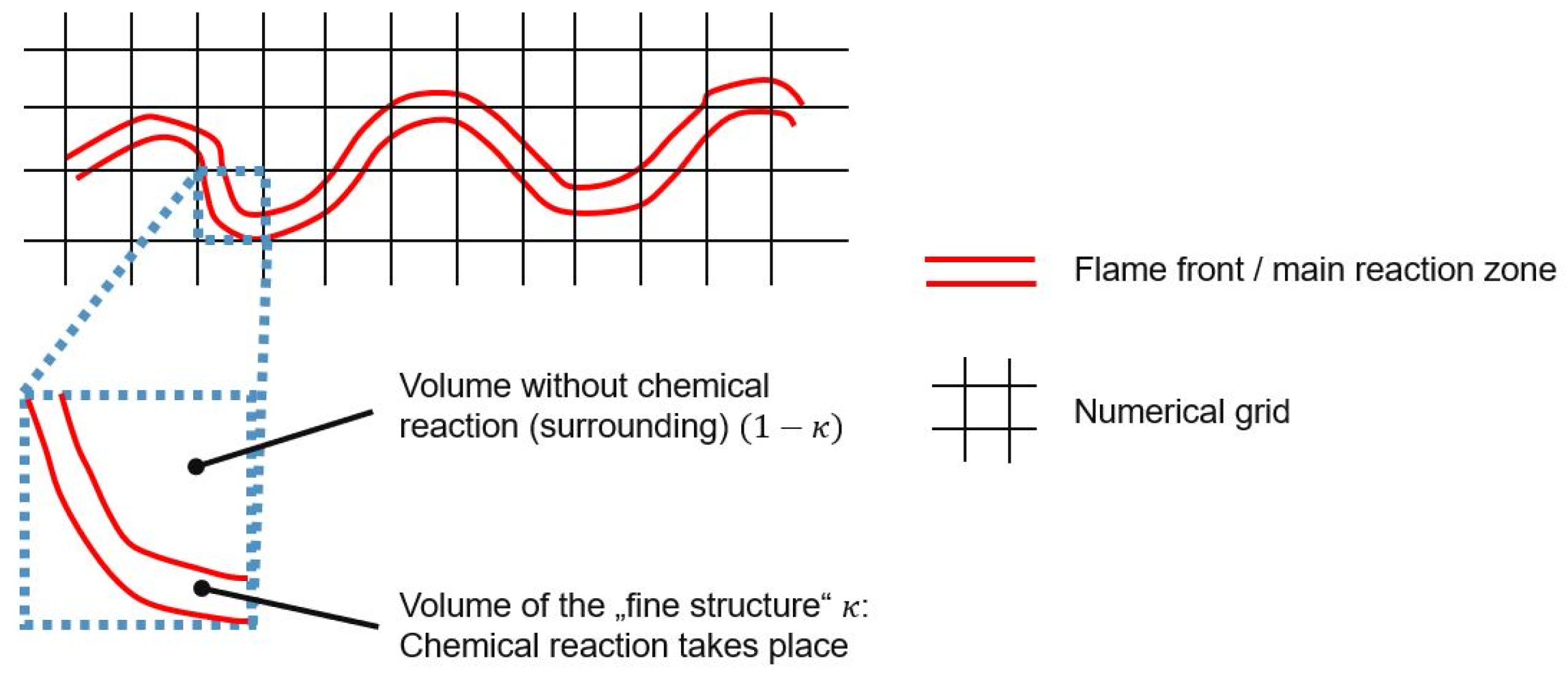
As explained in Section 2, the source term for each chemical species ${\dot{\omega }}_i$ has to be determined. Considering Equation (2), the volume fraction of the fine structure and the time scale will be determined based on the results from the turbulence models (turbulent kinetic energy, dissipation rate of the kinetic energy). However, the mass fractions in the fine structure after the fine structure time scale have to be calculated by the chemistry solver (integrating the chemistry). In the present study, reference simulations of all combustion cases (see Section 4) will be carried out using the “seulex” solver [42] in OpenFOAM, which is based on the linearly implicit Euler method with step size control [43]. For comparison, in Section 5, the simulations with this solver will be denoted as the “standard” chemistry (SC) solver.

For the prediction of the reaction kinetics within the fine structure of a numerical cell, a so-called reaction mechanism has to be chosen. In the reaction mechanism, the species involved in the chemical reactions, as well as the equations of the chemical reactions, are defined. So, for each reaction $j$, the reaction rate of a species $i$ can be calculated by Equation (11). In this equation ${\nu }_{i,j}^{\prime }$ and ${\nu }_{i,j}^{″}$ are the stoichiometric coefficients of the species $i$ at the reactant and the product side of the chemical equation, $k_{f,j}$ and $k_{f,j}$ are the reaction rate coefficients for the forward and backward direction of reaction $j$, and $\left[c_{k,j}\right]$ is the molar concentration of the species $i$ in the reaction $k$. Furthermore, $N$ stands for the overall number of species in the reaction mechanism, and ${\eta }_{k,j}^{\prime }$ as well as ${\eta }_{k,j}^{″}$ are the exponents forming the reaction order. In case of elementary reactions, the exponents are equal to the stoichiometric coefficients. The reaction rate coefficients can be derived by the Arrhenius equation (see Equation (12) as an example for a forward reaction). The Arrhenius approach includes the pre-exponential factor $A$, the temperature exponent $\beta$, the activation energy $E_A$, and the universal gas constant $R$.

$${\dot{\omega }}_{i,j}=\left({\nu }_{i,j}^{\prime \prime }-{\nu }_{i,j}^{\prime }\right)\left(k_{f,j}\prod _{k=1}^N{\left[c_{k,j}\right]}^{{\eta }_{k,j}^{\prime }}-k_{r,j}\prod _{k=1}^N{\left[c_{k,j}\right]}^{{\eta }_{k,j}^{\prime \prime }}\right)$$

(11)

$$k_{f,j}=A{T}^{\beta }{e}^{{\displaystyle \frac{-E_A}{RT}}}$$

(12)

The values used in Equation (12) can be found in the reaction mechanism. In the present study, the authors used a modified mechanism from Jones and Lindstedt (JL), which was optimized in the work by Frassoldati et al. [44]. All parameters of the reaction mechanism can be found in

Table 1. Reactions and Arrhenius parameters according to [44]. Units are cal, mol, L, and s.

	Reaction	$\mathit{A}$	$\mathit{\beta }$	${\mathit{E}}_{\mathit{A}}$
1	${CH}_4+0.5O_2\to CO+2H_2$	$3.06\times {10}^{10}$	$0$	$30\times {10}^3$
2	${CH}_4+H_{2}O\to CO+3H_2$	$3.84\times {10}^9$	$0$	$30\times {10}^3$
3	$CO+H_{2}O\rightleftharpoons {CO}_2+H_2$	$2.01\times {10}^9$	$0$	$20\times {10}^3$
4	$H_2+0.5O_2\rightleftharpoons H_{2}O$	$8.06\times {10}^{16}$	$-1$	$40\times {10}^3$
5	$O_2\rightleftharpoons 2O$	$1.5\times {10}^9$	$0$	$113\times {10}^3$
6	$H_{2}O\rightleftharpoons H+OH$	$2.3\times {10}^{22}$	$-3$	$120\times {10}^3$

.

Although more detailed reaction mechanisms are available in the literature with several hundreds or even thousands of species and reactions, a rather simple mechanism with 10 species and six chemical reactions was used. Other authors have already used more detailed mechanisms for the training of their ANNs (e.g., [6]). However, the applicability or feature space (temperature and species concentrations) is often limited (e.g., from 700 to 3100 K in DeepFlame). So, using a reduced reaction mechanism allows the training of the ANNs in the present study for a much wider range of the feature space without extensively increasing the size of the training data or training time. The size of the data for a detailed reaction mechanism for conventional natural gas combustion is already quite large. Extending the training data sets to different turbulence levels (affecting the time scale in the EDC), different fuel mixtures, and oxy-fuel combustion would lead to a large data size. Furthermore, important for an accurate prediction of the chemistry by the ANNs is that the AI-based method can handle the complexity of the reaction kinetics based on the high variation on the time scales and level of occurrence of some minor species. For example, in Table 1, it can be seen that reaction 6 is much faster than reactions 1, 2, or 3 by several orders of magnitude. Additionally, the reaction mechanism comprises major species, such as CH₄, with high concentrations (mass fractions) and minor species, such as OH, with low amounts. In between the major and minor species, several orders of magnitude also occur. These two aspects are the most critical parts for an accurate training of the ANNs and can be covered with the chosen reaction mechanism. The proposed training methodology described in the next sections should be applicable to larger reaction mechanisms, which will be worth investigating in future work.

3.2. Data Generation and Pre-Processing

There are several factors influencing the ANN’s capability to predict the behavior of a certain system. In addition to the training process itself, the quality of the training data is also essential. Inadequate data can lead to ANNs with a poor prediction capability. Thus, the present section focuses on how the data for the training was created and the pre-processing before the training procedure since these steps are of high importance for the later accuracy of the ANNs. In the first step, the range of the input feature space will be determined, as well as the required distribution of the data in this space. In the second step, the pre-processing of the data will be described, finally leading to data that allows the training of ANNs with high prediction accuracy.

To avoid the usage of chemistry solvers for the predictions of the species source terms ${\dot{\omega }}_i$, ANNs will be trained. It has to be mentioned that in the proposed framework, not the species source term ${\dot{\omega }}_i$, will be predicted directly from the ANN. Looking at Equation (13), the ANNs in the present study will calculate the source term ${\dot{\omega }}_{i,ANN}$. The multiplication with the fine structure volume fraction $\kappa$ is performed separately in OpenFOAM.

$${\dot{\omega }}_i=\rho {\kappa }_{new}{\displaystyle \frac{Y_i-Y_i^{\ast }}{{\tau }^{\ast }}}={\kappa }_{new}{\dot{\omega }}_{i,ANN}\left(\overrightarrow{x}\right)$$

(13)

The resulting network function to approximate the species source term ${\dot{\omega }}_i$ is denoted as ${\dot{\omega }}_{i,ANN}\left(\overrightarrow{x}\right)$ in Equation (13), where $\overrightarrow{x}\in \mathcal{X}$ represents the input feature space defined within the domain $\mathcal{X}\subseteq {\mathbb{R}}^n.$ Since the reaction rate of a species $i$ within a reactor (or fine structure) depends on the temperature, species concentrations, and residence time (fine structure time scale), the input feature vector can be defined as $\overrightarrow{x}=\left(\overrightarrow{Y},T,{\tau }^{\ast }\right)$. Subsequently, the vector for the species mass fractions is defined by all species involved in the reaction mechanism. During the CFD simulation, the input feature vector for the ANNs can be formed by the values from the previous iteration step $\left(\overrightarrow{Y},T\right)$, as well as the calculated time scale from the turbulence model, according to Equation (5) $\left({\tau }^{\ast }\right)$. It has to be mentioned that the pressure also affects the reaction rates and should be considered in the input feature vector. However, in the present study, the combustion takes place at ambient pressure without high gradients. Thus, the pressure is not part of the input feature space here.

For the supervised learning of the ANNs, corresponding outputs are necessary. For this purpose, the open-source software Cantera [7] was used. As mentioned in Section 2, the chemical reactions in the fine structures of a numerical cell can be approximated by a PSR or PFR. Due to the different modeling of the chemistry in the fine structures, the results of the two concepts also deviate from each other under the same initial conditions. When considering the fine structures as PSR, small eddies that arise on the surface or diffusion effects enable mass transfer with the environment of the main reaction zone. In the PFR, there is no mass transfer with the environment, and the reactions can be considered as isolated from the environment. Accordingly, the consideration as PFR leads to a higher mean reaction rate compared to the PSR since there is no back-mixing of reactants in the PFR. Bösenhofer et al. [45] indicate that modeling of the fine structures as a PFR provides good results under classical combustion conditions. If the focus is on a very detailed consideration of the reaction zone, the PSR approach should be chosen. Due to the lower numerical effort, the PFR approach was chosen for the data generation procedure with Cantera.

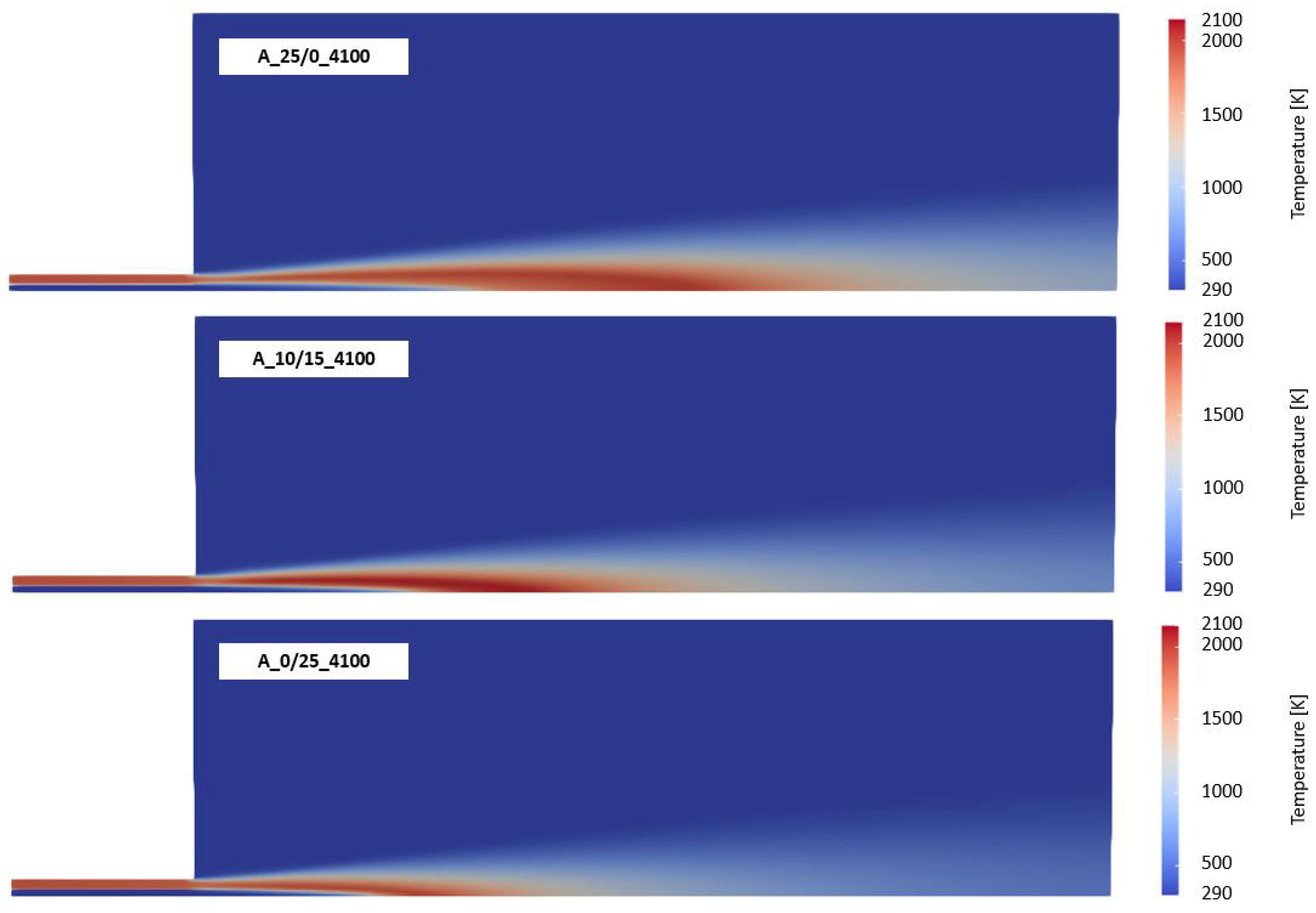
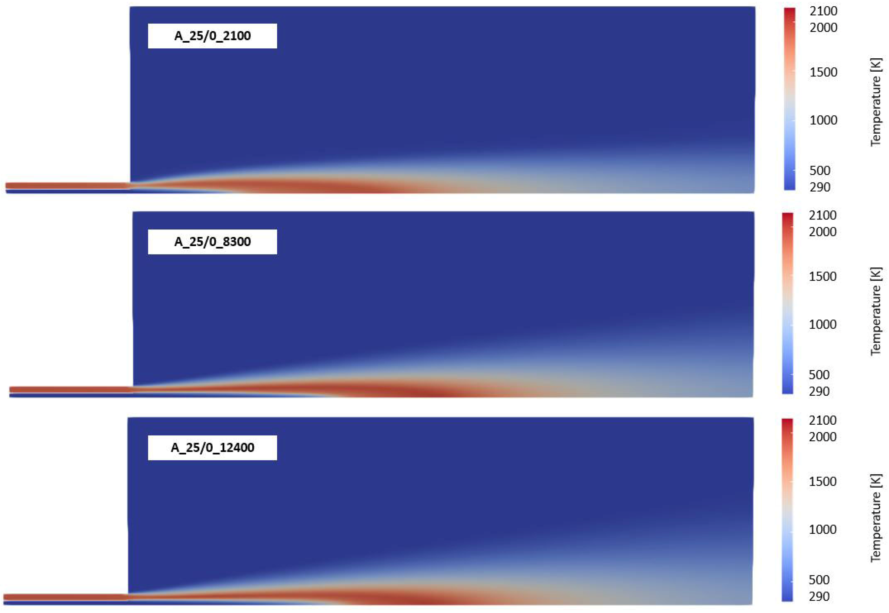
The PFR in Cantera is considered a 1D stationary tubular reactor with a constant cross-section and a constant flow rate. The fluid is considered to be homogeneous in the radial direction, and all diffusion processes in the radial and axial directions are neglected. Furthermore, the reactor is seen as operating under isobaric and adiabatic conditions. As an example, for the species concentrations over time (length) in the PFR, Figure 2 is shown below. The inlet conditions for the PFR can be seen as the species concentrations and temperature from the previous iteration step (conditions of the surrounding of the fine structure in the cell—$1-{\kappa }_{new}$). The horizontal axis in Figure 2 represents the residence time of the reactants in the PFR, which is equal to the fine structure time scale ${\tau }^{\ast }$, which means that with one PFR simulation, several input features of the time scale can be derived. If a PSR was used, a single simulation for each ${\tau }^{\ast }$ has to be carried out, which would have significantly increased the time for data generation. Based on the input features, temperature, and species concentrations, the species mass fractions in the fine structure $Y_i^{\ast }$ after the time scale ${\tau }^{\ast }$ can be determined. As a consequence, the network prediction (output feature) ${\dot{\omega }}_{i,ANN}\left(\overrightarrow{x}\right)$ can be formed in accordance with Equation (13).

To define the input feature space, OpenFOAM simulations with the standard chemistry solver were carried out for all considered combustion cases (see Section 4). During the simulations, the minimum and maximum values of all species concentrations, temperatures, and fine structure time scales were monitored. The observed maximum and minimum values were slightly extended to clearly avoid leaving the input feature space of the trained ANNs during the simulation. The range of each feature is shown in

Table 2. Range of the input features and distribution during Monte Carlo sampling for data generation with Cantera (based on Reiter [47]).

Feature	Minimum	Maximum	Distribution of Sampling
${\tau }^{\ast }$ [s]	0	0.1	Logarithmic
$T$ [K]	250	2600	Homogeneous
$Y_{O_2}$ [-]	0.0	1.0	Homogeneous
$Y_{H_{2}O}$ [-]	0.0	0.3	l
$Y_{{CH}_4}$ [-]	0.0	0.3	l
$Y_{CO}$ [-]	0.0	0.3	l
$Y_{{CO}_2}$ [-]	0.0	0.3	l
$Y_{N_2}$ [-]	0.0	0.8	-
$Y_{H_2}$ [-]	0.0	0.3	l
$Y_O$ [-]	0.0	0.005	s
$Y_H$ [-]	0.0	0.005	s
$Y_{OH}$ [-]	0.0	0.3	l

. It can be seen that the temperature range is from below 0 °C to 2600 K, which considers the full range of possible temperatures in the considered combustion cases. Also, the oxygen mass fraction is significantly extended to 1. Thus, oxy-fuel combustion can also be considered by the ANNs. In combustion with pure oxygen, the possible nitrogen mass fraction is reduced to 0. Within the ranges defined in Table 2, the input features were chosen by Monte Carlo sampling. Only nitrogen was determined by the fact that the sum of all mass fractions must be 1. In Table 2, the distribution of the feature sampling is also shown. For the time scale ${\tau }^{\ast }$, logarithmic sampling was chosen. This means that for the 30 samples of ${\tau }^{\ast }$ in one PFR simulation, more samples were defined for smaller time scales since the gradients of the species concentrations and temperature are higher. For larger time scales, the reaction moves towards equilibrium with low gradients. For the Monte Carlo sampling of the temperature and oxygen mass fraction, a homogeneous distribution of the random values was defined. The other distributions depend on whether the mass fractions of the species can reach larger values (l) or smaller values (s). For the species O and H (radicals), it can be seen in Table 2 that the maximum mass fractions are below 0.005. So, these species are defined as small (s) and the other ones as large (l).

For data generation, the input feature vector is formed by Monte Carlo sampling, which is quite clear for the time scale, the temperature, and the oxygen mass fraction. At first glance, it might be the case that the species mass fractions in all numerical cells during the OpenFOAM simulations are homogeneously distributed. For example, this can be seen in Figure 3 (left) by the purple area, highlighting the probability density of the mass fraction of CH₄. In the majority of the numerical cells, a very low mass fraction with an apparently Gaussian distribution is present. However, analyzing the results of the OpenFOAM simulations of all combustion cases showed that the mass fractions in all numerical cells of the simulation are not homogeneously distributed. After transformation of the species mass fractions using the Box–Cox transformation with $\alpha =0.1$ [48] according to Equation (14), the distribution looks clearly different (see Figure 3 (right)). Since the generated training data with Cantera should represent the “reality” (reference simulation with OpenFOAM) as well as possible, the distribution of the data sampling for the species mass fractions was defined as shown in

Table 3. Mass fractions and their corresponding possibility in the Monte Carlo sampling (based on Früh [49]).

$\mathbf{Range} \mathbf{of} \mathbf{Mass} \mathbf{Fraction} \mathbf{of} {\mathit{Y}}_{\mathit{i}}$	Probability [s]	Probability [l]
0.0–10−30	0.0005	0.0005
10−29–10−10	0.005	0.005
10−9–10−5	0.08	0.08
10−4	0.2425	0.08
10−3	0.2425	0.135
10−2–10−1	0.0	0.135

. It has to be mentioned that the data shown in Figure 3 were based on classes of the mass fractions, leading to a histogram plot. However, it was decided to convert the histogram to a line plot. Thus, in the line plot, negative values for the mass fraction can occur, which are based on interpolation between the classes near a mass fraction of 0. The data sets contain no negative mass fractions.

$$Y_{i,box-cox}\left(Y_i\right)=\left\{\begin{array}{c}{\displaystyle \frac{Y_i^{\alpha }-1}{\alpha }} if \alpha \ne 0,\\ \mathit{log}\left(Y_i\right) if \alpha =0.\end{array}\right.$$

(14)

In Table 3, six ranges for the species mass fractions were defined with a certain probability that the Monte Carlo sampling uses the specific range for the sampling. Considering the small mass fractions, it can be seen that most input features for these mass fractions will be generated from 10⁻⁴ to 10⁻³. For large mass fractions, the majority of the input data will be generated in a range of 10⁻³ to 10⁻¹, but very small mass fractions will also be considered during the sampling of the input features. With this sampling methodology for the input feature mass fraction, it is possible to generate training data, which is in close accordance with the “real” condition in the flame. Figure 3 (right) shows that the generated input feature for Cantera matches well with the OpenFOAM simulation data. Now, the input features cover the entire range for all combustion cases, and also the distribution of the features is in good agreement with “reality”. With these input features, Cantera simulations of the PFR will be performed.

Before the input and corresponding output data ${\dot{\omega }}_{i,ANN}\left(\overrightarrow{x}\right)$ can be used for the training of the ANNs, pre-processing steps have to be carried out. Data pre-processing is an important tool for improving the convergence of the training algorithm. For example, the data should be normalized to an order of magnitude of $\mathcal{O}\left(1\right)$ to prevent difficulties during the network training, which would lead to a lower learning rate for reasons of stability, and thus slow down the learning process [50]. It was proposed in [51] that training usually converges faster when the data is close to a standard normal distribution. If the underlying data is not normally distributed, the data should be brought into an order of $\mathcal{O}\left(1\right)$. For the normalization of the input and output data, Equation (15) (e.g., for species mass fraction $Y_i$) and (16) (for the reaction rates ${\dot{\omega }}_{i,ANN}$) were used. Both were normalized within a range of 0…1. Additionally, for the output data, a root function was used. With the root function, the output data fits the normal distribution much better.

$${\widehat{Y}}_i={\displaystyle \frac{Y_i}{Y_{i,max}}}$$

(15)

$${\widehat{\omega }}_{i,ANN}={\left[{\displaystyle \frac{{\dot{\omega }}_{i,ANN}}{{\dot{\omega }}_{i,ANN,max}}}\right]}^{1/3}$$

(16)

Finally, the pre-processed data set has a size of approx. 32 GB and consists of approx. 38 million data points

3.3. Subdivision of the Feature Space

The literature in Section 1 highlighted that using one ANN might not be feasible for the prediction of chemistry in the full range of input features. Several authors dramatically increased the number of ANNs in conjunction with a classification methodology (e.g., SOM in [27]). An alternative is given by the DeepFlame framework [6], which reduced the range for the input features for the single ANN trained for chemistry prediction. Prieler et al. [29] only trained two ANNs for the prediction of the chemical reactions in laminar counter-flow diffusion flames. The ANNs were trained for cases where ignition occurs and cases without ignition. Since this study revealed promising results with a limited number of ANNs, significantly reducing the training time, a similar approach was used in the present study. Volgger [52] stated that the applicability range for the separate ANNs can be related to the input feature of the temperature or the fine structure time scale. The temperature highly affects the reaction rates in the fine structure caused by the definition of the Arrhenius approach (see Equation (12)). However, the time scale was used as a criterion to determine which ANN should be used in the numerical cell for the prediction of the reaction kinetics.

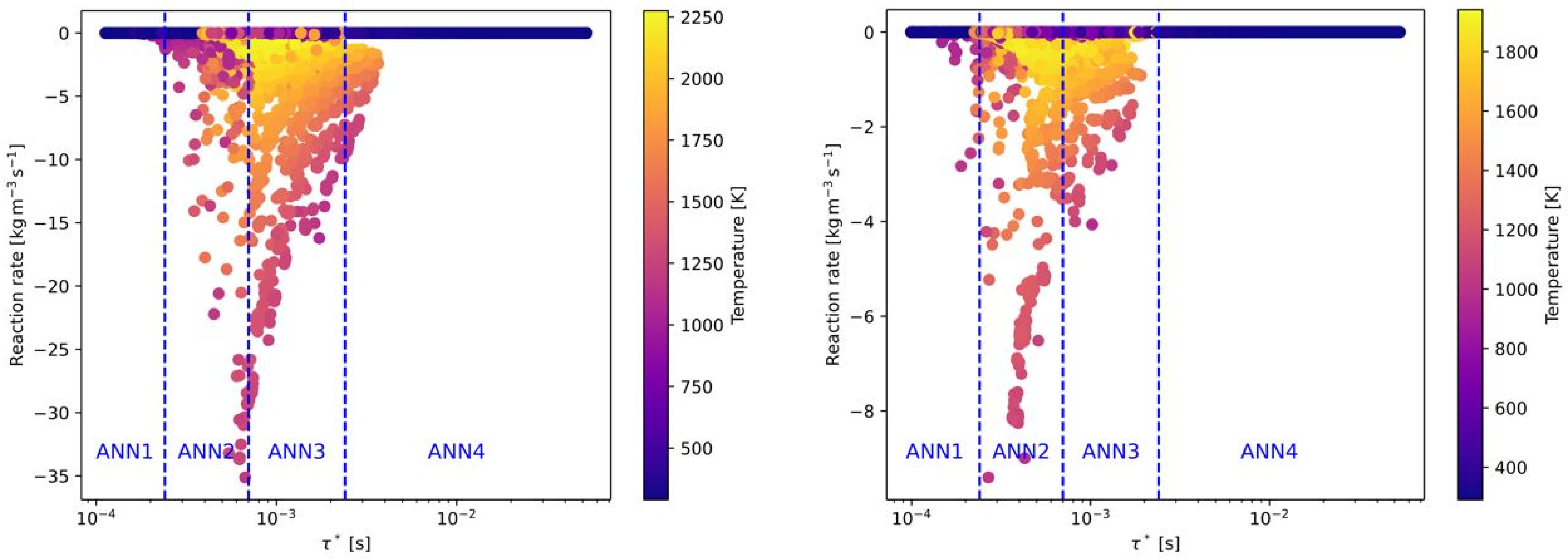
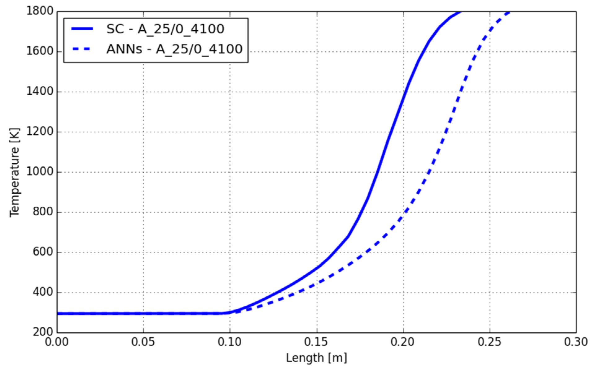
Four different ANNs were trained for pre-defined ranges of the fine structure time scale. In the following figures, the reaction rates of all OpenFOAM simulations were presented, depending on the fine structure time scale. The final regions of the time scale for each ANN (ANN1 to ANN4) are already marked in these figures and summarized in

Table 4. ANNs and their corresponding ranges for the fine structures’ time scales.

ANN	${\mathit{\tau }}_{\mathit{m}\mathit{i}\mathit{n}}^{\mathit{*}}$ [s]	${\mathit{\tau }}_{\mathit{m}\mathit{a}\mathit{x}}^{\mathit{*}}$ [s]
1	0	0.00024
2	0.00024	0.00055
3	0.00055	0.00117
4	0.00117	0.1

. In Figure 4, all reaction rates from the OpenFOAM simulations are presented for the combustion of CH₄ and H₂ with air. The reaction rates of these species were chosen because they are the main fuels in this study. The main target in defining the range of the time scale was that one or two ANNs should cover the range where it comes to combustion. The other ANNs should cover ranges without or with a minor number of combustion cases. This approach is similar to Prieler et al. [29]. In Figure 4, it can be seen that ANN2 and 3 cover the full range of the combustion cases with an equal distribution. ANN1 and ANN4 are considering time scales (nearly) without combustion. The highest reaction rates of CH₄ were found around a time scale of 0.0005 s⁻¹ and within a range of 0.0002 and 0.0011 s⁻¹. Thus, ANN2 and ANN3 were trained with data (input features) with these time scales. For the combustion of H₂, the maximum reaction rates occurred on a similar time scale (see Figure 4 (right)).

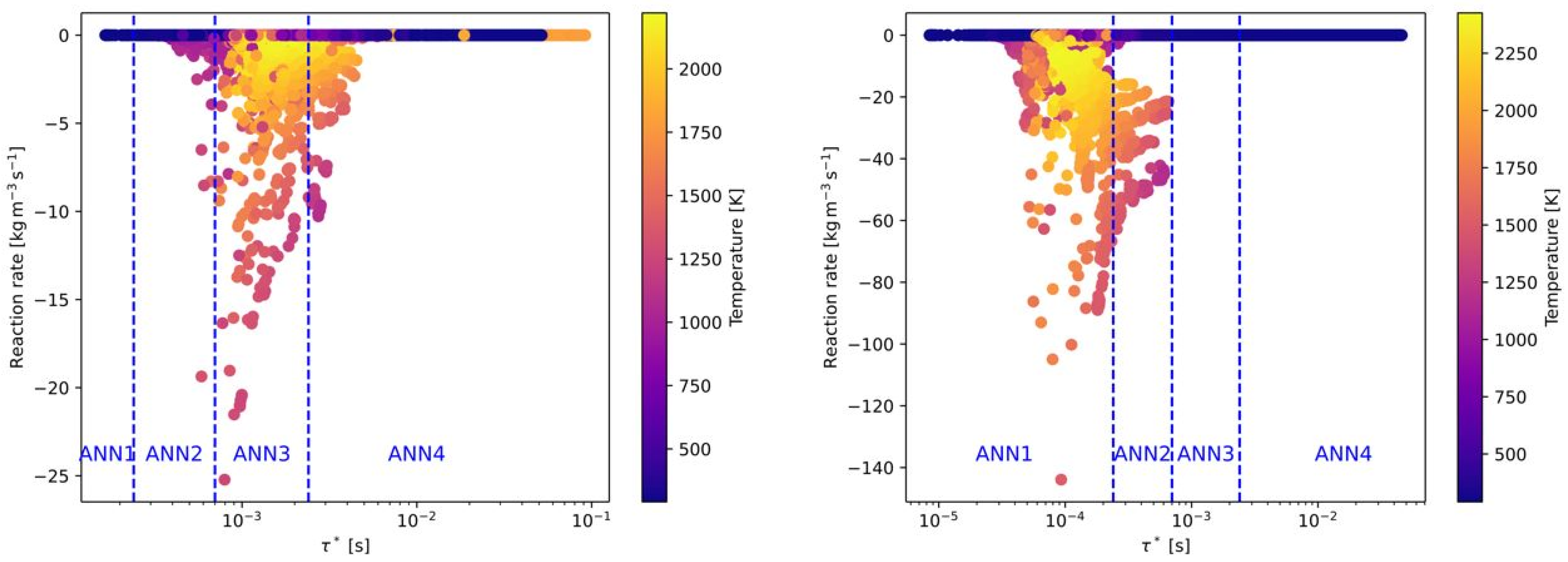
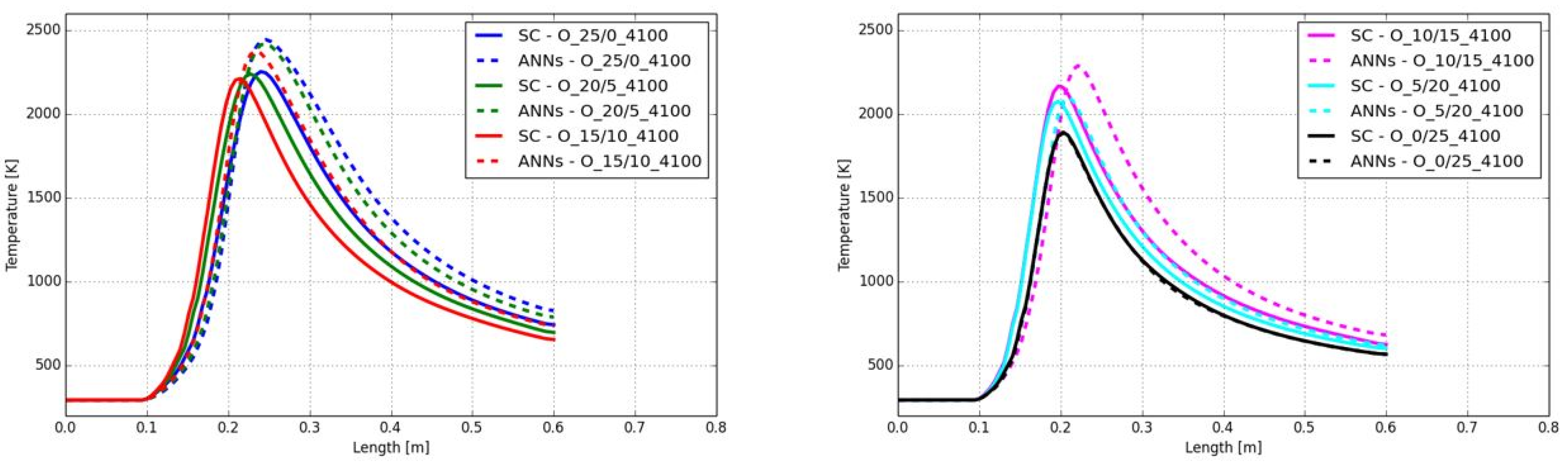
In Figure 5, the same combustion cases (CH₄ and H₂) in Figure 4 are presented, but with pure oxygen as an oxidizer instead of air (without nitrogen). Although the combustion with pure oxygen is in general related to a higher reactivity, the OpenFOAM data showed that the time scales are similar to the combustion with air as an oxidizer. Only a slight shift of the reaction rates to higher time scales can be observed. Therefore, the defined time scale ranges of the ANNs are also suitable for oxy-fuel combustion. It has to be mentioned that the values of the reaction rates between air-fuel and oxy-fuel combustion are clearly different for the combustion of CH₄ with air (see Figure 4 (left) and Figure 5 (left)). Whereas the maximum reaction rates with air are approximately 10 kg/(m³s), the reaction rates with oxygen are more than 3 times higher. This difference between air-fuel and oxy-fuel combustion cannot be observed when H₂ is used as fuel.

In addition to the composition of the fuel and oxidizer, the third effect to be covered by the ANNs is the level of turbulence. As described later in Section 4, six Reynolds numbers, related to the flow conditions in the main jet of the burner, were investigated. In Figure 6, the effect of the Reynolds numbers on the reaction rates and time scales for the combustion of CH₄ with air is presented. Compared to Figure 4 (left), the time scale, where the highest reaction rates occurred, was shifted slightly to higher time scales (see Figure 6 (left)). Thus, all cases with ignition are now located in ANN3. In contrast, higher turbulence in the main jet significantly decreases the time scales for high reaction rates. As a consequence, all burning cases are now in the range of ANN1. Similar to air-fuel and oxy-fuel combustion of different fuels (see Figure 4 and Figure 5), there is hardly any difference in the time scales when switching from air-fuel (see Figure 6) to oxy-fuel combustion (see Figure 7) under different turbulence levels. But, the maximum reaction rate increases again when oxy-fuel is used as an oxidizer instead of air.

Finally, the analysis using the OpenFOAM simulation data showed that the time scale is only affected by the turbulence levels. The effect of the fuel mixture and the oxidizer is minor. However, the oxidizer significantly affects the level of the maximum reaction rates. Thus, it can be concluded that the turbulence level had an effect on the ranges of the fine structure time scales for the different ANNs, but it had no effect on the other training parameters or data pre-processing steps.

For the air-fuel and oxy-fuel combustion cases with all fuel types, ANN1 was mainly used for higher Reynolds numbers when an ignition case was considered. With a decreasing turbulence level in the main jet, ANN1 is replaced by ANN2 and ANN3. For larger time scales, ANN4 is applied, which represents cases without ignition for all cases. In Table 4, the ranges of the time scales for each ANN are summarized. Although OpenFOAM data were used to roughly determine the ranges of the residence times, the exact values shown in Table 4 were determined by trial and error. The best performance was achieved with the ranges presented in Table 4. But, it has to be mentioned that the differences between the trials were very small.

3.4. ANN Structure, Training, and Hyperparameter Tuning

In the present study, a feed-forward architecture without backward connections was used for the ANNs. This approach seems reasonable since all previous studies mentioned in Section 1 also used the same architecture. The ADAM algorithm was used as the learning algorithm for all ANNs trained in this work. According to Kingma et al. [53], this is a computationally efficient and robust stochastic optimization algorithm that is particularly suitable for problems with large data sets and many parameters. From the entire data set, 80% was used for training and 20% for validation. Also, other ratios between training and validation data sets were tested with a negligible effect on the performance of the ANNs. The learning rate is adjusted individually for different parameters, whereby the change in learning rates is also monitored using a weighted moving average. The batch size for the learning process has a significant effect on the generalization ability of the neural network. In general, the larger the batches, the worse the network generalizes. This means that the prediction quality of the network on a validation data set decreases (see, for example, [54]). On the other hand, larger batches have the advantage that the calculation per iteration step can be better parallelized, which greatly reduces the training time. In the present study, the batch size was defined with a value of 256, and the training duration was 100 epochs. It was observed that after 100 epochs, the error was at a minimum level for all ANNs without a hint of over-fitting. Using smaller batch sizes had a minor effect on the training errors shown in

Table 5. Errors during ANN training using different sizes for the data set.

Size of Data Set	MAE	MSE	RMSE
2	0.097	1.018	0.346
4	0.082	0.912	0.288
8	0.059	0.478	0.221
16	0.055	0.345	0.196
32	0.051	0.333	0.191

but led to a higher training duration. Thus, the value of 256 was a good compromise.

To determine the structure of the ANNs with regard to the number of hidden layers and the number of neurons per layer, a hyperparameter tuning was carried out. The Keras tuner [55] in TensorFlow [56] was used to select suitable hyperparameters. Bayesian optimization was used to search for a set of hyperparameters that best approximates the data set. In the course of this work, an ANN structure of four hidden layers with 256 neurons per layer proved to be a good compromise between training effort and network performance for the tested ANNs. In addition to the four hidden layers, an input layer with 12 neurons (10 species, fine structure time scale, and temperature) and an output layer with 10 neurons (reaction rate for each species ${\dot{\omega }}_{i,ANN}$) was used. The rectified linear unit (ReLU) was used as the activation function for the neurons of the input layer and the hidden layers. This function is suitable for training very deep neural networks with a large number of hidden layers [57]. An alternative activation function would be the Gaussian error linear unit (GELU), as it was used in the DeepFlame framework. A comparison between the ReLU and GELU was not performed in the course of the present study. A linear activation was applied to the output layer. Although for the training of the final ANNs the size of the data set was 32 GB, smaller data sets were tested, and the errors were observed (see Table 5).

The coupling of the ANNs, which are based on Python v3.11.10, with the C++ framework of OpenFOAM v11, was performed via the pybind11 library [58].

4. Test Setup

4.1. Basis Configuration

To test the performance of the trained ANNs compared to the SC solver in OpenFOAM, a test setup according to Figure 8 was chosen. The burner is based on the Sandia flame [59] but operated under different conditions to achieve stable simulations with the numerical setup described in Section 2 and Section 3. The diameter of the inner annulus (main jet) was 7.2 mm, and the inner and outer diameters of the pilot jet were 7.7 and 18.9 mm. In the main jet, a premixed fuel/air mixture is provided to the combustion area. To stabilize the main reaction zone (flame), a pilot jet is arranged with a gas composition in accordance with the Sandia flame D (see

Table 6. Operating conditions of the flame in the basis configuration.

		Main Jet	Pilot Jet	Co-Flow
Temperature [K]		294	1880	291
Velocity [m/s]		10.0	5.0	0.9
Volume fraction [%]	${CH}_4$	25	0	0
	$CO$	0	0.40	0
	${CO}_2$	0	6.92	0
	$H$	0	0.07	0
	$H_2$	0	0.18	0
	$H_{2}O$	0	14.50	0
	$N_2$	58	72.66	0.79
	$O$	0	0.13	0
	$O_2$	17	4.68	21
	$OH$	0	0.46	0

). The co-flow jet has a diameter of 300 mm, providing air to the combustion domain. Additionally, the length of the combustion domain was 60 cm. The numerical grid used for the simulation with OpenFOAM is presented in Figure 9 and consists of 5170 cells.

The test setup shown in Figure 8 will be operated under different fuel compositions, air-fuel and oxy-fuel combustion, and different turbulence levels (based on the Reynolds number in the main jet). Since the geometry of the burner is the same in all simulations, the operating conditions have to be changed. The basis configuration of the burner (basis operating conditions) is shown in Table 6, which is similar to the Sandia flame D, except for the inlet velocities for the main and pilot jets. The simulation results obtained with these settings are denoted as “basis” in Section 5.

The basic configuration (basic operating conditions) of the burner presented in this section can be seen as air-fuel combustion with a Reynolds number of 4100 and a fuel mixture in the main jet of 25 vol% CH₄ and 0 vol% H₂.

4.2. Variation of the Oxidizer (Air-Fuel and Oxy-Fuel Combustion)

In oxy-fuel combustion, all of the nitrogen is removed from the oxidizer, which means that only pure oxygen is supplied to the combustion. In contrast to air-fuel combustion with nitrogen in the oxidizer (commonly 79 vol% nitrogen and 21 vol% oxygen in the oxidizer), nitrogen must not be heated up. Thus, more energy is released from the chemical reactions and is available to heat up the reaction products. As a consequence, higher flame temperatures can be reached, also affecting the reaction kinetics. In this study, all considered combustion cases were tested under air-fuel and oxy-fuel conditions.

Although there is also nitrogen in the pilot jet, the composition of the gas inlet there was not changed, and nitrogen is still present there. The reason for that is the high temperature of the pilot jet of 1880 K, leading to the fact that nitrogen only absorbs a minor fraction of the heat released by the combustion process. Thus, the majority of the energy is still for heating up the combustion products. Therefore, the composition of the pilot jet has not changed from air-fuel to oxy-fuel conditions.

In

Table 7. Volume fraction of nitrogen and oxygen for air-fuel and oxy-fuel conditions.

		Main Jet		Co-Flow
		Air-Fuel	Oxy-Fuel	Air-Fuel	Oxy-Fuel
Volume fraction [%]	$N_2$	17	75	21	100
	$O_2$	58	0	79	0

, the change in the gas compositions for the main jet and the co-flow when switching from air-fuel to oxy-fuel combustion is shown.

4.3. Variation of the Fuel Mixture

For these combustion cases, the composition of the fuel mixture in the main jet was varied. To ensure that there are no effects due to different degrees of turbulence, the Reynolds number remains constant in all configurations. The initial configuration with a Reynolds number of 4100 in the main jet was defined as the basis (see Section 4.1). Since both the density and the viscosity of the mixture in the main jet change when the fuel composition changes, the velocity in the main jet must be adjusted in order to keep the Reynolds number constant. The sum of the volume fractions of CH₄ and H₂ in the main jet was 25 vol% in the basis configuration (see Table 6). This value should be constant when changing the fuel mixture in the main jet. The velocities at the burner inlet for the flame under different turbulence levels are summarized in

Table 8. Velocities at the burner inlets for the different fuel mixtures under air-fuel conditions in [m/s].

Vol. Frac. Ratio $\raisebox{1ex}{${\mathit{C}\mathit{H}}_4$}\!\left/ \!\raisebox{-1ex}{${\mathit{H}}_2$}\right.$	25/0	20/5	15/10	10/15	5/20	0/25
Main jet	10.0	10.3	10.5	10.8	11.1	11.5
Pilot jet	5.0	5.0	5.0	5.0	5.0	5.0
Co-flow	0.9	0.9	0.9	0.9	0.9	0.9

and

Table 9. Velocities at the burner inlets for the different fuel mixtures under oxy-fuel conditions in [m/s].

Vol. Frac. Ratio $\raisebox{1ex}{${\mathit{C}\mathit{H}}_4$}\!\left/ \!\raisebox{-1ex}{${\mathit{H}}_2$}\right.$	25/0	20/5	15/10	10/15	5/20	0/25
Main jet	9.2	9.4	9.6	9.8	10.1	10.4
Pilot jet	5.0	5.0	5.0	5.0	5.0	5.0
Co-flow	0.9	0.9	0.9	0.9	0.9	0.9

.

4.4. Variation of the Degree of Turbulence

In these tests, the flow velocities of the main jet and the pilot jet were adjusted based on the initial configuration in order to generate different turbulence levels. The ratio of velocities is 2:1 between the main jet and the pilot jet. The composition of the fuel mixture remains constant with 25 vol% CH₄ and 0 vol% H₂. The velocities for changing the turbulence levels are presented in

Table 10. Velocities at the burner inlets for the different turbulence levels under oxy-fuel conditions in [m/s].

Reynolds Number	Main Jet	Pilot Jet	Co-Flow
2100	5.0	2.5	0.9
4100 (basis)	10.0	5.0	0.9
6200	15.0	7.5	0.9
8300	20.0	10.0	0.9
10,300	25.0	12.0	0.9
12,400	30.0	15.0	0.9

.

4.5. Naming of the Different Combustion Cases

Since there are a lot of different combustion cases, at this point, the naming will be explained, which will be later used in Section 5. First, at the beginning of the name, the oxidizer is highlighted. If the case is an air-fuel case, the name starts with the letter “A”. Otherwise, the letter “O” is used. The second part of the naming represents the fuel mixture, which is just the ratio of the volume fraction between CH₄ and H₂ (see Table 8 and Table 9). At the end, the Reynolds number is given. For example, when the combustion case oxy-fuel with a Reynolds number of 4100 and 15 vol% CH₄ in the fuel is considered, the label in a chart would be “O_15/10_4100”.

5. Results

In this section, the simulation results with the standard chemistry (SC) solver and the ANNs will be compared and analyzed. In Section 5.1, the effect of the fuel composition on the combustion behavior will be presented for both numerical approaches. The same procedure is given in Section 5.2 for the different degrees of turbulence. The analysis will be carried out on the basis of the predicted temperatures, mass fraction of CO, and the calculation time, which was observed on a simple notebook with an Intel i7-4720HQ CPU and 16 GB DDR3L-RAM (1600 MHz). Only one CPU core was used to avoid the effects of the parallelization procedure in this study.

5.1. Effect of the Fuel Composition

In this section, the combustion cases with air-fuel combustion (Section 5.1.1) and oxy-fuel combustion (Section 5.1.2) are presented.

5.1.1. Air-Fuel Combustion

In Figure 10, the contour plots of the temperature predicted with the ANNs are shown for air-fuel combustion at a Reynolds number of 4100. The fuel composition was changed in accordance with Table 8. It can be seen that the length of the flame is decreasing with higher H₂ content in the fuel stream instead of CH₄. Although the plots in Figure 10 are from the simulation with ANNs, the length of the flame is also decreasing with the SC solver in a similar way. An increasing maximum flame temperature can be observed when the fuel mixture is mixed with more hydrogen, replacing CH₄. However, when hydrogen completely replaces the methane, the maximum flame temperature drops.

In addition to Figure 10, Figure 11 shows the temperatures along the center line of the burner. Considering the case A_25/0_4100 (blue lines), it can be observed that the ANNs predicted a delay in the temperature increase in the flame, as well as slightly over-predicted the maximum flame temperature. Due to the delay in the temperature increase, the position of the peak temperature is shifted from 35 cm (SC) to 36 cm (ANN) (distance from fuel inlet). The temperature was over-predicted by 71 K.

Adding hydrogen to the fuel mixture leads to an increase in the delay of the temperature increase. For example, in the case A_10/15_4100 (magenta), the shift on the peak temperature was from 23 cm (SC) to 27 cm (ANN) (delta of 4 cm). In contrast, the values of the peak temperatures are in a much better agreement between the SC and the ANNs with a difference of 2 K. When only hydrogen was used as fuel in the main jet, the prediction of the ANNs fits very well with the SC approach, with a difference of the peak temperature shift and peak temperature value of 5 mm and 13 K.

The resulting temperatures showed that the ANNs predicted a slight error on the position where the temperature starts to increase for CH₄ combustion, as well as the peak temperature, which was over-predicted by the ANN. Only small amounts of hydrogen in the fuel mixture significantly increase the accuracy of the predicted maximum temperature, with maximum deviations of approx. 15 K.

A similar behavior was detected for the CO mass fractions along the burner axis. The same delay, observed on the temperature increase, can be seen on the CO mass fraction as well (see Figure 12). The shift of the maximum mass fraction was comparable to the temperature shift in Figure 11. Although there was the same shift in the position of the maximum CO mass fraction, the maximum values were well predicted with the ANNs. The maximum difference on the CO mass fraction was observed in the case A_10/15_4100, with a value of 0.004.

Despite the deviation on the maximum temperature of 71 K in the case A_25/0_4100, the maximum temperatures and CO mass fractions were in good agreement between the SC and ANNs. However, the shift in the position of the maximum temperature and start of the temperature increase was found in all cases, except for hydrogen in the case A_0/25_4100. This indicates that the calculated reaction rates at a lower or near ambient temperature level are significantly under-predicted by the ANNs. This can be seen in Figure 13, where below 800 K, the steep increase in the temperature calculated by the SC cannot be covered by the ANNs. Above 800 K, the slope of the temperature increase is the same with the SC and ANNs, which indicates that the ANNs are working correctly. The DeepFlame framework neglected temperatures below 700 K and used the SC for the chemistry calculation in this temperature range. This would be an option for the present framework, too. The reason for this lack of accuracy between the high-temperature and low-temperature regions (<800 K) is caused by the sudden change between input features, which leads to chemical reactions (combustion) and input features where no chemical reactions occur. If in a numerical cell the boundary conditions (e.g., species mass fractions, temperature, residence time) lead to a chemical reaction, in other words, if ignition occurs, it is hard to predict for a single ANN since there is a sudden jump from low temperatures to combustion, leading to high temperatures. This fact was already shown in Prieler et al. [29]. Since all four ANNs are covering the entire temperature range, a lack of accuracy can be determined. An alternative approach, based on the four ANNs, can increase the accuracy and is later shown in Section 6.

Nevertheless, the average calculation time of the six CFD simulations in the present section was 500 min (SC) and 35 min (ANNs). This means a reduction in the calculation time with one CPU core of a factor of 14.

5.1.2. Oxy-Fuel Combustion

In Figure 14, the contour plots of the temperature are presented under oxy-fuel conditions and different fuel mixtures. The Reynolds number was fixed at 4100. From the contour plots, it can be observed that the flame length is decreasing with increasing hydrogen content. The same was found with the maximum flame temperature.

In the air-fuel cases in Section 5.1.1, a delay in the temperature increase was observed in all cases. For the oxy-fuel cases shown in Figure 15, the delay at low temperatures is minor, leading to an accurate prediction of the position of the maximum temperature by the ANNs. For example, the shift in the position for the case with methane as fuel (case O_25/0_4100) was 6 mm. The highest shift was found in the case of O_10/15_4100 with 2 cm. Although the position of the flame was well predicted, the values of the maximum temperatures were over-predicted by the ANNs. The highest over-prediction was found for the combustion of methane with a difference of 191 K. Similar to the air-fuel cases, the deviation on the peak temperature was decreasing, finally resulting in close agreement for the combustion of hydrogen (case O_0/25_4100).

The over-prediction of the temperature in some oxy-fuel cases is caused by the limited number of input features covering high oxygen mass fractions and higher temperatures during the training procedure of the ANNs since these input features are located at the boundaries of the defined input feature range (see Table 2). Thus, increasing the input feature range or the number of training samples at the boundaries of the input feature range would be beneficial for the accuracy in oxy-fuel cases.

In Figure 16, the CO mass fraction along the center line of the burner is presented. The small shift from the temperature plots in Figure 15 is also observable in the CO charts. In contrast, the difference in the peak temperature cannot be observed in the peak CO mass fraction. In all combustion cases, the peak CO mass fraction fits well and can be accurately predicted by the ANNs.

In all oxy-fuel combustion cases with different fuel mixtures, the position of the flame was well predicted with a maximum shift in its position of 2 cm between the SC and ANNs. Furthermore, the shape of the flame with the ANNs was in close accordance with the prediction from the SC approach. A higher error was observed on the peak temperature, which was significantly over-predicted by the ANNs.

The average calculation time for the simulation of all combustion cases in this section was 420 min (SC) and 35 min (ANNs), which is a reduction in the calculation time by a factor of 12. The simulations were carried out with one CPU core.

5.2. Effect of the Degree of Turbulence

In this section, the combustion cases with air-fuel combustion (Section 5.2.1) and oxy-fuel combustion (Section 5.2.2) are presented at different turbulence levels.

5.2.1. Air-Fuel Combustion

Figure 17 shows the contour plots of the temperatures predicted by the CFD simulation using ANNs. Starting with the lowest degree of turbulence (a Reynolds number of 2100 in the main jet), a short flame with a maximum temperature of approx. 1800 K can be determined. Increasing the Reynolds number leads to a longer flame and slightly higher flame temperature of up to approx. 2000 K. Despite the flame length, the shape is similar in all cases.

In Figure 18, the combustion case A_25/0_2100 resulted in the shortest flame, reaching the peak temperature at 29 cm. Although the Reynolds number of the main jet was continuously increasing above a Reynolds number of 4100, the position of the maximum peak temperature hardly changed. Also, the value of the peak temperature was similar. Considering the case with the lowest Reynolds number, the temperature trend along the burner axis was well predicted by the ANNs. The comparison with the SC showed negligible errors. For example, the position of the maximum temperature showed a deviation between the ANNs and the SC of 0.2 mm, and the predicted maximum temperatures were 1870 K (ANNs) and 1863 K (SC), respectively. The highest deviation between the ANNs and SC was observed for a Reynolds number of 4100, which was already discussed in Section 5.1.1, with its shift on the position of the flame and the over-prediction of the flame temperature of 71 K. Using Reynolds numbers between 8300 and 12,400 in the main jet led to a close accordance of the temperature between the ANNs and SC. So, the shape and the peak temperatures were well predicted for all cases with varied turbulence levels.

The CO mass fractions along the burner axis are presented in Figure 19. All mass fractions predicted by the ANNs showed a good agreement with the SC solver, despite the delay of the start of the increase for a Reynolds number of 4100 (compare Figure 18 and Section 5.1.1). Only the peak CO mass fractions are higher when the Reynolds number is at 6200 or higher. Here, the maximum peak CO mass fraction’s difference was detected for the combustion case A_25/0_8300. The ANNs predicted a maximum value of 0.105, and the SC determined the maximum value as 0.116. All other differences along the burner axis were significantly lower.

In contrast to the different fuel mixtures, the change in the Reynolds number hardly affects the accuracy of the ANN’s prediction. The trends of the calculated temperatures and CO mass fractions overall were in good agreement with the standard chemistry (SC) solver. The advantage of the ANNs was clearly highlighted by the comparison of the calculation time, which was reduced by a factor of 12 for all the cases in the present section.

5.2.2. Oxy-Fuel Combustion

The oxy-fuel combustion with different fuel mixtures in Section 5.1.2 showed that the ANNs can predict the flame shape in good agreement with the standard chemistry solver. However, the peak flame temperature was over-predicted. In the present section, the Reynolds number was changed, but the fuel mixture was the same in all cases with 25 vol% CH₄ and 0 vol%H₂. In Figure 20, the contour plots of the simulated temperatures with the ANNs are shown for Reynolds numbers of 2100, 8300, and 12,400. It can be seen that with a higher Reynolds number, the flame length increases. Furthermore, the flame temperature reaches a temperature of approx. 2500 K when the Reynolds number was at the maximum of all investigated cases.

As mentioned in the last paragraph, the shape of the oxy-fuel flames with different fuel mixtures was well predicted by the ANNs; the same behavior was found for changing degrees of turbulence (see Figure 21). The shape of the flame, as well as the position of the maximum temperature, was well predicted. For example, at a Reynolds number of 2100, the position of the peak temperature was at 19.7 mm (SC) and 19.1 mm (ANNs), respectively. For the highest Reynolds number, the peak temperature was at the same position. Only at a Reynolds number of 4100 was the position shifted. The reason was already described in the previous sections. The start of the temperature increase showed a delay when the ANNs were used instead of the SC. This means that the predicted source terms in low-temperature regions were under-predicted by the ANNs. In addition to the shape and position of the flame, the value of the peak temperature was over-predicted in all cases, which is similar to the cases in Section 5.1.2 (Reynolds number of 4100 and different fuel mixtures).

In Figure 22, the CO mass fractions along the burner axis are shown for the different Reynolds numbers. The position of the peak CO mass fraction was in good agreement with the SC model, despite the shift at a Reynolds number of 4100. This was already confirmed by the temperature plots in Figure 21. In contrast to the calculated peak temperature, the peak CO levels were similar between the SC and the ANNs. At higher Reynolds numbers, the used ANNs showed a high accuracy. Again, a simulation speed-up of a factor of 12 was determined.

5.3. Comparison with DeepFlame

The presented approach showed the capability of feed-forward ANNs to predict the reaction rates in reactor-based modeling of flames within CFD simulations. Since the introduction showed that ANNs were already used in the past for this task, a short comparison with the DeepFlame framework will be given. Similar to the present methodology, DeepFlame uses a single feed-forward ANN with the GELU activation function. However, the ANN was only used for temperatures above 700 K. For cell temperatures below, the SC solver was used. In contrast, the presented methodology used four ANNs, which covered the full range of conditions in the entire computational domain (also temperatures below 700 K). Since the working range of DeepFlame is slightly limited, a comparison of the accuracy of both methods is barely possible. It was pointed out in the sections above that the accuracy of the prediction is highly related to the ANN results at low temperatures, which define when the combustion starts. Unfortunately, DeepFlame only considered the low-temperature region with the SC solver instead of the ANN. The results from the last sections showed that the four ANNs, in some cases, under-predicted the reaction rates at lower temperatures, leading to an ignition delay compared to the SC. However, after the first increase in the temperature, the four ANNs were able to predict the temperature trend and CO mass fractions in close accordance with the SC. Considering the calculation time, DeepFlame was able to reduce the overall calculation time (flow + chemistry, etc.) by a factor of 15 on an AMD EPYC 7402 system with an NVIDIA GeForce 3090. In the present study, an Intel i7-4720HQ CPU with 16 GB DDR3L-RAM (1600 MHz) was used. However, for the calculation, only one CPU core was active to avoid parallelization effects. A mean speed-up factor of 12 was observed, which is comparable to DeepFlame.

6. Discussion, Conclusions, and Outlook

In the present paper, artificial neural networks were used to predict the chemical source terms in combustion modeling to accelerate the simulation compared to the standard chemistry solver in OpenFOAM. For the first time, machine learning techniques were applied to determine the chemical source terms in CFD simulations of flames with different fuel mixtures, turbulence levels, and air-fuel/oxy-fuel combustion. In the proposed methodology, the four different ANNs were trained for different ranges of the fine structure time scale to be more precise for the full range of input features (temperature and species concentrations) instead of using a single ANN with limited accuracy. The simulations were carried out with OpenFOAM and the standard chemistry (SC) solver in OpenFOAM as reference. To determine the accuracy of the ANNs, they were implemented in the OpenFOAM framework, replacing the SC solver. Subsequently, the simulations were carried out again. The simulation results between the SC solver and the ANNs were compared, and the following observations were made:

• A significant calculation speed-up for all combustion cases was detected when the SC was replaced by the ANNs. The mean speed-up factor was determined by a value of 12 (only one CPU core was used to avoid parallelization effects). It has to be mentioned that only a small reaction mechanism with 10 species and six reactions was used. According to Cuoci et al. [9], when conventional chemistry solvers are applied, the calculation time for the chemical reactions increases nearly quadratically (approx. 1.9) with the number of species. Considering more detailed mechanisms with the ANNs would require more time for ANN training, but the prediction time for the source terms should be very similar to the present case. This reveals the very high potential of ANNs in combustion modeling.
• For the air-fuel combustion cases, the flame shape as well as the peak temperature levels were well predicted for all Reynolds numbers. However, at a Reynolds number of 4100 in the main jet, the position of the flame was shifted downstream by about 4 cm. It was concluded that the ANNs under-predicted the chemical source terms in the low temperature region (below 800 K). For the other Reynolds numbers, the ANN’s prediction was of high accuracy.
• In air-fuel combustion at a Reynolds number of 4100, a shift in the flame position was observed, and a change in the fuel mixture towards a higher hydrogen content led to more accurate predictions. This means that ignition (temperature increase) starts earlier with higher hydrogen content and shows better agreement with the SC.
• In oxy-fuel combustion, the position of the flame and shape for all cases were well predicted by the ANNs. However, the flame’s peak temperature was significantly over-predicted in all oxy-fuel cases with approx. 100–200 K.
• In addition to the temperature, the CO mass fraction in the flame was also monitored. It was found that the shift of the CO mass fraction along the burner axis was in close accordance with the temperature shift. However, the peak CO values were always in good agreement with the SC solver’s prediction for all Reynolds numbers, fuel mixtures, and air-fuel/oxy-fuel.

It can be concluded that the proposed methodology can predict the chemistry in flames for a wide range of operating conditions with high accuracy. The determined calculation speed-up reveals the potential of the ANNs for large-scale industrial furnaces, where the calculation time is still high. Thus, the optimization of industrial combustion systems in the metal, glass, etc., industries using CFD simulations can be achieved in a shorter timeframe in the future. Since future research in industrial combustion systems is focused on the optimization and novel furnace designs, it is essential to carry out a fast and accurate CFD simulation. For example, Prieler et al. [60] investigated an industrial steel reheating furnace (about 18 MW), including the transient heating of the steel billets. The CFD simulation (including the combustion process, radiative heat transfer, and coupling between the gas phase and solid materials) took about 10 days to fully converge. It can be seen that detailed investigations or parameter studies for different furnace operating conditions or designs would take a significant amount of time, and there are even larger combustion systems in operation in industry. Reducing the calculation by a factor of 12 will help future research in this field. Additionally, modern combustion systems are facing a rapid trend to multi-fuel operation, where the fuel mixture as well as the oxidizer can be different between the burners inside one system. For example, Mayr et al. [61] investigated a pusher-type furnace where burners were operated with pure oxygen as well as with 25 vol% oxygen in the oxidizer at the same time. Thus, it is important that the ANNs can handle a wide range of operating conditions to be used in modern industrial furnaces.

Nevertheless, the proposed framework still lacks accuracy in the low-temperature region and in oxy-fuel cases. For this purpose, the future work will use an additional ANN that is only trained with data, where temperatures below 800 K are used as input features but for the entire range of the fine structure time scales (see Figure 23). This means that the entire data set will be sub-divided into two regions, one above 800 K and one below. The data set for temperatures below 800 K will be used to train only a single ANN. In contrast, the data sets for temperatures above 800 K will be further sub-divided into four ANNs since this methodology worked well to predict the flame shape in the present study. However, no changes to the data pre-processing or training methodology will be performed in a future study. For the over-prediction in the oxy-fuel cases, more data samples on oxy-fuel combustion for the training of the ANNs should be introduced. This will certainly affect the data generation process, leading to a higher number of Cantera simulations.