Motor Fault Diagnosis and Predictive Maintenance Based on a Fine-Tuned Qwen2.5-7B Model

Abstract

The rapid growth of electric vehicle requires more rigid safety and reliability requirements for EV motors. But traditional methods struggle to deal with complex conditions, small samples, and cross-dataset generalization. Thus, we propose a framework using a fine-tuned Qwen2.5-7B model for EV motor fault diagnosis and predictive maintenance. It merges current and vibration signals, extracting features via time–frequency analysis to assess the health state of motor. Lightweight fine-tuning with LoRA and QLoRA reduces training costs and improves generalization and real-time capabilities. Experiments show a 96.5% accuracy on single datasets, 91.2% across conditions, and 82.7% with small samples, outperforming CNN and LSTM models. This analysis not only highlights key features like vibration spectral energy and current fluctuation amplitude, but also enhances the interpretability of results. This study introduces a novel approach to EV motor fault diagnosis, demonstrating the great potential of large language models to tackle fault diagnosis of EV motor.

1. Introduction

With the optimization of the global energy structure and the accelerated promotion of “carbon peak and carbon neutrality” goals, electric vehicles (EVs) are gradually replacing traditional fuel vehicles, becoming an important component of future intelligent transportation and green mobility. In the core system of EVs, the drive motor, as the key component providing power, directly affects the vehicle’s acceleration performance, driving range, and driving safety. Once the motor fails, it is highly likely to cause power loss and system paralysis, and even pose risks to personnel and property safety. Therefore, efficient and intelligent motor fault diagnosis and predictive maintenance technologies for EVs have become a crucial technical link in the new energy vehicle industry to ensure operational safety and enhance user experience.

In recent years, although significant progress has been made domestically and internationally in the field of motor fault diagnosis, relevant research primarily revolves around signal analysis and pattern recognition. This includes monitoring and feature extraction methods based on sensor data like current, vibration, and temperature, as well as intelligent classification algorithms represented by machine learning and deep learning [1]. These technologies can achieve the identification and classification of typical faults in laboratory environments and obtain relatively accurate diagnostic results in specific scenarios, initially promoting the practical application of intelligent operation and maintenance for EVs. However, from the perspective of industrial implementation, existing technologies still face a series of challenges in engineering practice that cannot be ignored, mainly manifested in the following aspects.

Firstly, complex signal sources and drastic changes in operating conditions: EV motors typically operate in dynamic environments with high speeds, high loads, and variable frequency, exhibiting significant non-stationarity and diversity in their signals. For example, under the influence of factors such as different slopes, accelerations, temperature environments, and road types, there are huge differences in the patterns of motor current and vibration signals, causing drastic fluctuations in the signal’s time–frequency structure. Traditional diagnostic methods relying on single-modal features struggle to stably extract representative fault features, leading to significant fluctuations in model output during operating condition switching, making reliability difficult to guarantee.

Secondly, a lack of high-quality labeled data: Unlike mature fields like computer vision, the probability of EV motor failure during actual operation is relatively low, and most faults exhibit a slow evolution process, making it difficult to collect complete fault evolution data in a timely manner. Meanwhile, the complex structure and numerous operating parameters of motors mean that obtaining accurately labeled fault type information often relies on expert experience and disassembly analysis, which is not only costly but also susceptible to subjective factors. Most existing datasets suffer from problems such as small sample sizes, class imbalance, and non-standardized fault labels, severely limiting the generalization performance and robustness of models [2].

Thirdly, diagnostic methods are overly reliant on specific scenarios and equipment. Currently, most studies build diagnostic systems based on a single device for model design and data collection, heavily relying on sensor types, sampling frequencies, and operating parameters. When the model is applied to other vehicle models or sensor configuration environments, significant differences in input data format or feature space often lead to a sharp decline in recognition accuracy, or even complete failure. This strong dependence on equipment and data sources severely limits the generalized deployment and cross-platform promotion of motor fault diagnosis technology [3].

Additionally, some advanced models based on deep learning, such as Convolutional Neural Networks (CNNs), Recurrent Neural Networks (RNNs), and Long Short-Term Memory (LSTM) networks, despite having good feature extraction capabilities and advantages in temporal modeling, still face practical bottlenecks like large model parameter sizes, a high dependence on sample data for training, and low inference efficiency [4]. This makes them difficult to deploy directly on resource-constrained edge devices, limiting their real-time diagnosis and edge intelligence deployment capabilities. Against this background, academia and industry are urgently seeking a novel diagnostic method with stronger generalization ability, lightweight deployment capability, and adaptability to small samples. Among these, large language models (LLMs), due to their significant advantages, demonstrated across semantic understanding, knowledge transfer, and structured reasoning, are gradually becoming a potential breakthrough for the evolution of intelligent industrial diagnostic technology [5].

In summary, although the field of EV motor fault diagnosis has achieved phased progress, it still faces three core challenges that urgently need to be overcome.

• Insufficient Cross-Condition Adaptability: During actual operation, EV motors often operate under variable working conditions, such as different speeds, loads, temperatures, and environmental noise. Research indicates that traditional models heavily depend on specific operating conditions during the training phase. Once conditions change, models face the “data distribution shift” problem, making it difficult to maintain diagnostic accuracy in new environments. For instance, Su et al. (2022) pointed out that most models built on shallow features are extremely sensitive to signals under low-speed, high-load, or high-temperature environments, exhibiting a limited generalization ability [6]. Although recent studies have attempted to enhance model robustness through data augmentation and domain adaptation techniques, they still require substantial manual intervention and parameter tuning, and their adaptability to abnormal conditions remains insufficient, making true end-to-end cross-condition transfer difficult to achieve [7].
• Weak Small-Sample Learning Ability: In practical applications, obtaining large amounts of high-quality motor fault data presents numerous challenges. On the one hand, the probability of severe failures in EV motors during the early stages is low, making real fault samples scarce. On the other hand, labeling costs are high, and manual diagnostic experience is difficult to standardize. This forces most research to model small-sample or class-imbalanced datasets, leading to a severe risk of overfitting for deep learning models. Although some studies have tried introducing few-shot learning [8], transfer learning, or Generative Adversarial Networks (GANs) [9] to simulate fault samples, diagnostic accuracy under small-sample conditions still struggles to meet industrial application requirements due to limitations in prior knowledge and model instability [10].
• Limited Cross-Dataset Generalization Ability: The collection of motor fault data is often constrained by differences in specific equipment models, sensor layouts, and sampling frequencies, leading to structural inconsistencies between different datasets. Currently, most models require rebuilding the feature extraction process and retraining the model for each new dataset, lacking a unified modeling mechanism. This “model reconstruction” not only increases deployment costs but also limits the model’s transferability and universality. Wang et al. (2023) pointed out in their research that the accuracy of traditional CNN or LSTM architectures drops sharply during cross-platform and cross-sensor data transfer, revealing the vulnerability of existing models in adapting to heterogeneous data [11].

In summary, the three major challenges faced by EV motor fault diagnosis—cross-condition adaptation, small-sample data, and cross-dataset generalization—have become key bottlenecks hindering the practical implementation of intelligent diagnostic systems. To address this, this paper attempts to leverage the powerful semantic modeling and generalization capabilities of large language models, proposing an EV motor fault diagnosis and predictive maintenance framework based on a lightweight fine-tuned Qwen2.5-7B large model. The main innovations of this method include the following:

• Constructing a multimodal fusion semantic representation mechanism that transforms the time-frequency features of current and vibration signals into structured text input, enabling Qwen2.5 to perform fault identification by leveraging its natural language modeling advantages;
• Applying low-rank fine-tuning strategies such as LoRA and QLoRA to achieve efficient adaptation by updating only a small number of parameters, significantly reducing the dependency on large-scale samples and computational power;
• Designing a sliding window mechanism and temporal context modeling strategy, equipping the model with dual capabilities for short-term fault judgment and medium-to-long-term trend prediction.

Our experimental results show that, across multiple typical industrial data scenarios, the proposed method outperforms traditional deep learning methods in terms of accuracy, stability, and generalization ability, providing a theoretical basis and engineering pathway for realizing intelligent diagnostic systems with true industrial practical value.

2. Related Work

2.1. Research Status of EV Motor Fault Diagnosis

As the core driving component, the fault diagnosis of electric vehicle (EV) motors has long been an important research direction in the field of intelligent operation and maintenance. Current research primarily focuses on fault pattern recognition methods based on sensor signals such as current, vibration, and temperature, covering signal analysis techniques from the time domain and frequency domain, to the time–frequency domain, such as Fourier transform, wavelet analysis, and envelope demodulation. Early studies mostly combined traditional machine learning algorithms like Support Vector Machines (SVMs) and Random Forests (RF) to achieve automatic identification of typical faults (e.g., bearing damage, rotor imbalance, stator winding short circuits) under laboratory conditions [11]. However, with the increasing complexity of actual EV operating scenarios, existing methods have gradually revealed issues in three aspects: First, models perform poorly in cross-condition environments, struggling to cope with data distribution shifts caused by changes in actual operating conditions like load, speed, and temperature. Second, models strongly depend on large-scale labeled samples, whereas high-quality, comprehensive fault data are difficult to obtain in real-world scenarios, leading to severe overfitting and poor generalization during training [12]. Third, most existing models rely on specific equipment or sensor configurations, making it difficult to adapt them to cross-platform deployment requirements.

To address these challenges, existing research has made improvements in several directions. For example, to tackle the adaptability issues caused by varying operating conditions, researchers have proposed cross-condition transfer learning methods based on domain adaptation, such as Multi-Scale Domain Subspace Alignment Convolutional Neural Network (MS-DSACNN) and Time-Spectrum Domain Adaptation Network (TSDAN) [13], achieving feature transfer from source to target operating conditions [14]. For the small-sample problem, Generative Adversarial Networks (GANs) are widely used to synthesize fault data to augment training sets, while meta-learning methods enhance rapid adaptation capabilities in scenarios with scarce data by learning shared knowledge across tasks [15]. In comparison to cross-dataset generalization, Dynamic Multi-Adversarial Adaptation Network (DMAAN) and Multi-Branch Domain Adaptation Network (MBDAN) [16] improve the transfer generalization ability of models across heterogeneous data by constructing domain-invariant feature subspaces [17]. Although the above methods solved existing problems in some respects, they generally suffer from issues like reliance on complex parameter tuning, high computational cost, and confused adaptation processes. Based on this context, introducing LLMs with strong generalization capabilities has become a significant breakthrough in the research.

2.2. Application of Multimodal Sensors in Industrial Predictive Maintenance

Multimodal perception offers significant advantages in intelligent fault diagnosis, especially in EV scenarios, where fusing sensor data such as current, vibration, and temperature can more comprehensively reflect the motor’s operating status [18]. Multimodal fusion can be categorized into data-level fusion, feature-level fusion, and decision-level fusion, with feature-level fusion being the most widely used in practical applications. For example, Gao et al. enhanced the model’s ability to identify compound fault types by concatenating and fusing the time-frequency features of current and vibration signals [19]. In early fusion, raw or low-level features from different modalities are directly concatenated and input into the model, which has advantages in extracting global information; whereas late fusion processes information from different modalities through multiple branch networks separately and then fuses them at the high-level decision layer, suitable for tasks where modal features differ significantly. In recent years, some studies have also introduced attention mechanisms to achieve weighted fusion, dynamically allocating feature weights among multiple modalities to further enhance the sensitivity and robustness of fault diagnosis. However, multimodal fusion still faces challenges such as poor data synchronization and inter-modal redundant interference, requiring more efficient and interpretable fusion strategies to support large-scale industrial deployment.

2.3. Typical Applications of Deep Learning Models in Temporal Signal Analysis

In mechanical equipment health monitoring, deep learning, with its end-to-end feature learning capability, has gradually replaced traditional feature extraction methods that rely on manual experience [20]. Particularly in the field of EV motor fault diagnosis, Convolutional Neural Networks (CNNs) are widely used for classifying time–frequency images due to their excellent spatial feature extraction capabilities, while Recurrent Neural Networks (RNNs) and their variants like LSTM and GRU excel at handling temporal dependency structures, enabling the mining of trend changes and subtle anomalies in time series signals like current and vibration. For example, An et al. proposed an LSTM-based rolling bearing fault diagnosis method that effectively captures long-range dependencies in historical vibration data [21], while Zhang et al. significantly enhanced the coupling modeling capability between multimodal features by constructing a multi-channel CNN-Transformer model [22]. Despite the significant progress in accuracy achieved by these methods, they are highly dependent on large amounts of labeled data, have large model parameter sizes, high training costs, and lack a sufficient cross-dataset generalization ability, limiting their direct deployment in multi-source heterogeneous data environments.

2.4. Research Progress on Large Models in Industrial Cross-Modal Tasks

In recent years, LLMs have demonstrated powerful knowledge transfer and context modeling capabilities in natural language processing and cross-modal learning. Domestically developed open-source models represented by Qwen2.5 have achieved excellent performance in tasks such as Chinese–English semantic understanding and multi-turn reasoning, possessing broad industrial adaptability. In industrial scenarios, the application of LLMs has expanded from text-based question answering to complex reasoning tasks in temporal data. For example, Sun et al. applied Qwen2.5 to coal mine risk prediction scenarios, achieving automatic identification and causal analysis of hidden risk patterns by structurally converting multimodal sensor data into language descriptions [23]. Tao et al. proposed the idea of textualizing vibration time-series features in bearing fault diagnosis tasks and fine-tuned LLMs using LoRA and QLoRA strategies, significantly enhancing the model’s adaptability under cross-condition and cross-dataset scenarios [24]. Furthermore, researchers have combined the attention mechanisms of LLMs with prior fault knowledge bases to achieve interpretable reasoning about fault causes, making diagnostic results more understandable and engineering-feasible. These achievements indicate that models like Qwen2.5 possess significant advantages in structured perception, multimodal fusion, and cross-scenario generalization, pointing out new directions for building next-generation intelligent diagnostic systems [25].

2.5. Research Gaps and Innovations of This Work

Despite numerous research advancements in the field of EV motor fault diagnosis in recent years, particularly in multimodal fusion, deep learning modeling, and the preliminary application of LLMs, existing research still faces innovation gaps in three key aspects.

Firstly, the representation methods for multimodal data are not unified, and their semantic fusion capabilities are insufficient. Current mainstream methods mostly adopt feature-level or decision-level fusion strategies. Although these can enhance the model’s perception of complex operating conditions, there is still a disconnect in processing the temporal and structural semantics of physical signals like current and vibration. There is currently a lack of a high-level semantic understanding mechanism capable of transforming multimodal time-frequency features into a unified learnable representation, thereby achieving stronger cross-modal feature linkage and diagnostic interpretation. Secondly, the adaptability of deep models to small samples and new operating conditions remains inadequate. Although existing research has attempted to improve model learning capabilities in data-scarce situations through methods like meta-learning, transfer learning, or GANs, these methods generally suffer from high computational costs, complex parameter tuning, and limited generalization ability, making it difficult to adapt to the frequently changing working conditions and data environments in actual industrial deployments. Thirdly, existing cross-dataset generalization research mostly focuses on feature space alignment, lacking a universal semantic representation mechanism. For example, methods like MSATM and DMAAN, although capable of achieving a certain degree of cross-domain transfer, often rely on large amounts of source domain data for retraining, providing insufficient support for cold starts in the target domain, and failing to achieve true “zero-shot” or “few-shot” fault diagnosis generalization. Meanwhile, although LLMs like Qwen2.5 show good potential in semantic understanding and cross-modal modeling, their integration methods, fine-tuning strategies, and feature input structures in industrial fault diagnosis scenarios lack systematic exploration, limiting their application efficiency and deployment feasibility, especially for smaller versions of the model.

Based on the above shortcomings, the research framework proposed in this work aims to address the following three key deficiencies: Regarding the lack of a unified mechanism for feature textualization and multimodal semantic fusion, this paper proposes converting the time–frequency features of current and vibration signals into structured language representations, leveraging the LLM’s text data modeling capabilities to achieve cross-modal understanding [26]. Meanwhile, addressing the conflict between small-sample adaptation ability and training overhead, low-rank fine-tuning strategies like LoRA and QLoRA [27] are introduced, updating only a small number of parameters to reduce training resource requirements while maintaining a high adaptability [28]. Finally, addressing the absence of a unified generalization framework for cross-condition and cross-dataset scenarios, a universal diagnostic model architecture capable of processing data across conditions, devices, and sensors is constructed through a unified language input space and shared contextual representation [29].

Therefore, this paper innovatively proposes a fault diagnosis and predictive maintenance framework integrating feature textualization, multimodal semantic enhancement, and lightweight fine-tuning techniques [30]. It applies Qwen2.5 to the task of EV motor intelligent O&M for the first time, systematically constructing an LLM adaptation mechanism and application paradigm oriented towards industrial scenarios, providing a new paradigm and feasible path for the practical application of large language models in industrial intelligent diagnosis.

3. Proposed Method

The proposed framework for EV motor fault diagnosis and predictive maintenance based on fine-tuned Qwen2.5 mainly includes five key modules: data acquisition, signal processing and feature extraction, multimodal data fusion, Qwen2.5 model fine tuning, and real-time fault diagnosis and prediction. The entire process is illustrated in Figure 1. The hardware and software platform are built based on a GPU environment, primarily using the Python programming language 3.14 and the PyTorch framework v2.5.0 for model training and validation to ensure efficient data processing and rapid model iteration.

The multimodal data used in this paper mainly include current and vibration signals. Current sensors and vibration sensors are installed near the motor stator and bearings, respectively, to capture abnormal signals during motor operation. Data acquisition covers different load, speed, and temperature conditions to comprehensively evaluate the model’s generalization ability. Fault types are labeled on the collected data using expert knowledge and historical data, including normal operation, bearing damage, winding short circuits, etc.

3.1. Feature Construction and Fine-Tuning Dataset Construction

3.1.1. Multimodal Signal Feature Extraction

In this study, we utilize current and vibration signals collected during EV motor operation for fault diagnosis. These signals consist of discrete time-series data collected by sensors, which differ in format from the natural language text typically processed by LLMs. To fully leverage the powerful semantic information processing capabilities of LLMs, we extract features with clear physical meaning that reflect the motor’s health status from these raw signals and transform them into textual descriptions suitable for LLM input [1,2,3,4,5,6,8,9,10,15].

Our approach involves systematically extracting a set of time domain and frequency domain features from both current and vibration signals. These features aim to quantify the statistical properties and structural patterns of the signals in different dimensions, providing a basis for the LLM to understand and diagnose motor faults. Necessary preprocessing is performed on the collected current and vibration signals to eliminate noise and artifacts. This may include filtering, detrending, or segmenting the signals into appropriate windows to ensure the accuracy of subsequent feature extraction. For both current and vibration signals, we calculate a series of standard statistics that reflect the signal’s amplitude distribution and temporal structure. Common time-domain features include:

• Mean: Represents the average value of the signal.
• Standard Deviation: Measures the dispersion of signal values.
• Root Mean Square (RMS): Represents the effective value of the signal.
• Skewness: Assesses the asymmetry of the signal distribution.
• Kurtosis: Assesses the tail characteristics of the signal distribution.
• Peak Value: The maximum absolute value in the signal.
• Crest Factor: The ratio of the peak value to the RMS value.
• Shape Factor (Form Factor): The ratio of the RMS value to the mean of the absolute values.
• Impulse Factor: The ratio of the peak value to the mean of the absolute values.

These features capture the overall energy, variability, and impulsiveness of the signal, which are crucial for identifying different fault conditions. To capture the spectral characteristics of the signals, we employ advanced time-frequency analysis techniques, such as the Wavelet Synchrosqueezed Transform (WSST), to process the signals. WSST provides high-resolution time-frequency representations suitable for capturing the frequency components of non-stationary signals. From these representations, we extract the following frequency-domain features:

• Spectral Mean: The average value of the spectrum.
• Spectral Variance: The dispersion of spectral values.
• Spectral Skewness: The asymmetry of the spectral distribution.
• Spectral Kurtosis: The peak of the spectral distribution.
• Frequency Centroid (Gravity Frequency): The weighted average frequency.
• Frequency Standard Deviation: The dispersion of the frequency distribution.
• Root Mean Square Frequency (RMSF): The effective frequency.
• Specific Frequency Band Energy Ratio: The proportion of energy within frequency ranges relevant to fault characteristics.

These frequency domain features reveal the main frequency components and energy distribution of the signal, crucial for identifying specific fault types. By integrating features from both current and vibration signals, we construct a comprehensive feature set that enhances diagnostic capability, potentially capturing fault characteristics that might be missed by single-modality signals. The extracted numerical features are subsequently converted into structured natural language descriptions, for example, ‘The mean value of the current signal is 0.021 A’ or ‘The spectral energy of the vibration signal is 1.5 × 10⁻³’. This textualization step makes the data compatible with the input requirements of Qwen2.5, which is designed to process and understand natural language, thereby effectively integrating signal data with the LLM framework. In summary, the multimodal signal feature extraction process includes preprocessing the signals, calculating diverse time domain and frequency domain features from current and vibration data, and converting these features into a text format suitable for LLM processing. This approach ensures that the LLM can effectively utilize its language understanding capabilities to diagnose motor faults based on multimodal data.

3.1.2. Fine-Tuning Dataset Construction and Feature Textualization

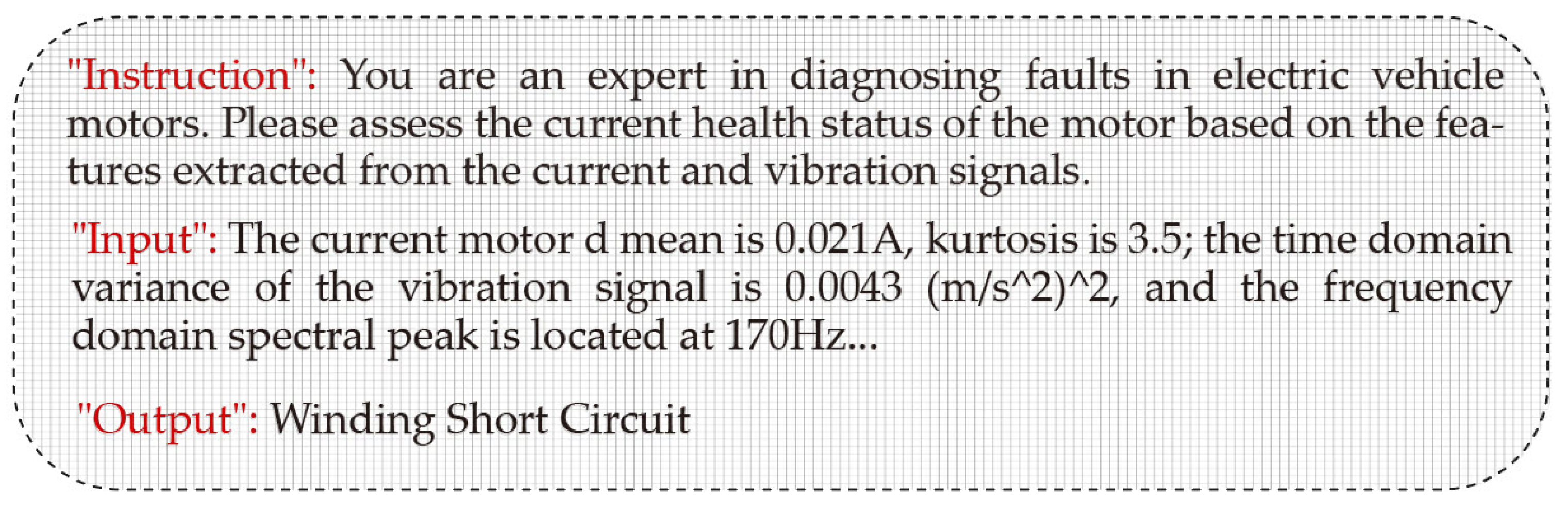
After extracting the multimodal features mentioned above, the crucial step is to transform them into a format that the LLM can understand and process. We adopt a strategy of feature textualization, converting numerical feature vectors into structured natural language descriptions, rather than directly inputting raw numerical values into the model. During the feature description generation process, the feature values extracted from each sample are combined with their corresponding feature names, such as current signal mean value, vibration signal variance etc., to form a descriptive text passage.

Then, question–answer pairs are constructed in a format of instruction–input–output. The generated feature description text serves as the input of model, and the corresponding motor health status or fault mode e.g., Normal, Bearing Damage, Winding Short Circuit, etc. serves as the output of model. Simultaneously, a clear task ‘instruction’ is set, informing the model that it needs to perform fault diagnosis based on the features of input. In this way, each sample constitutes a question–answer pair for Supervised Fine-Tuning (SFT). A typical example is shown as following in Figure 2.

The feature textualization approach allows for the retention of original numerical values and units in the input, thus avoiding the loss of physical meaning that might occur with mandatory normalization. It should be emphasized that the conjunctions and sentence structures in the input text are primarily intended to help the LLM understand the task and the meaning of the data, and do not need to strictly follow fixed templates built upon extensive expert knowledge. The core objective is to enable the model to understand the diagnostic task and the structure of the input data, rather than relying on specific wording.

3.2. Lightweight Fine-Tuning Diagnostic Framework Based on Qwen2.5

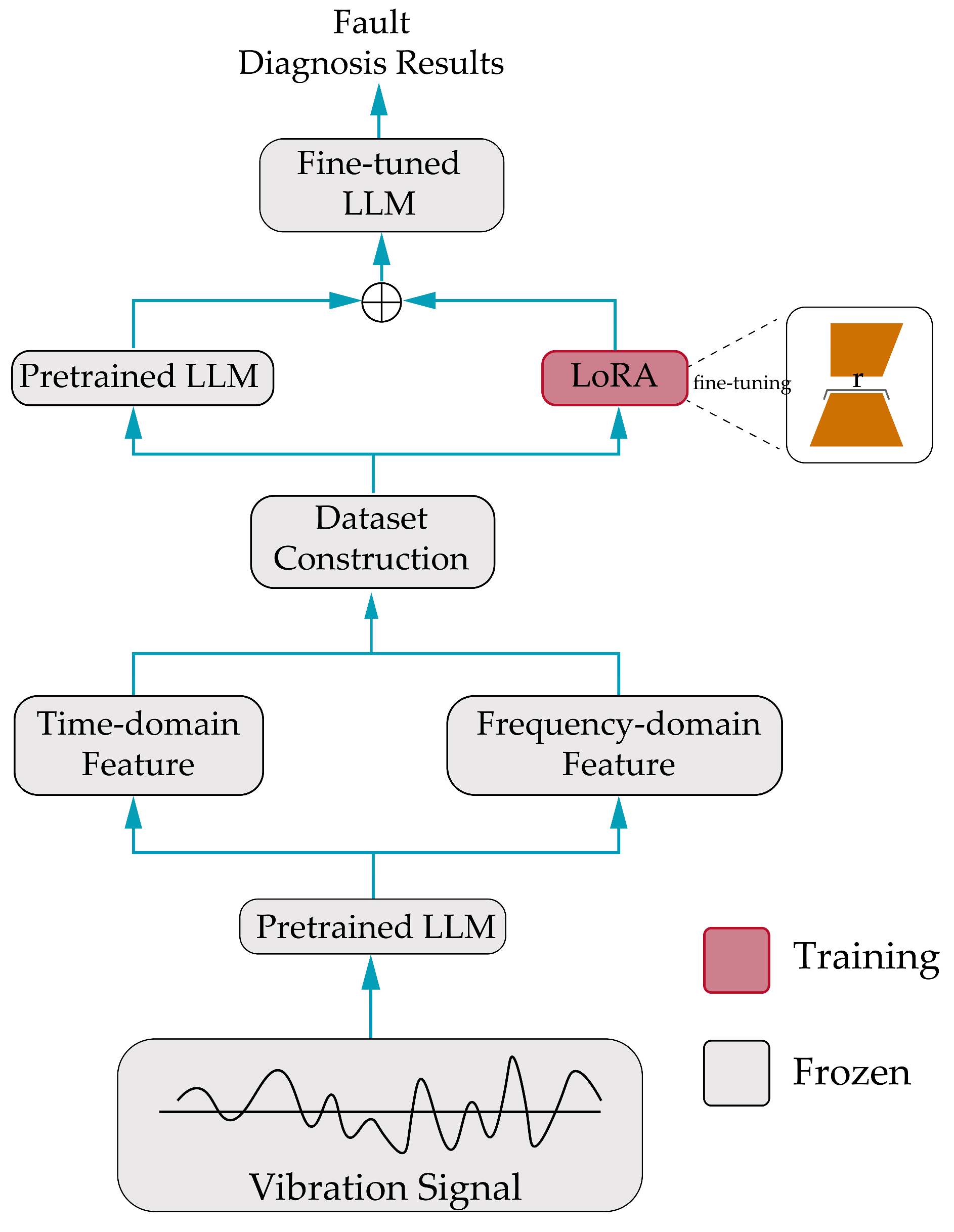
To adapt the Qwen2.5 large language model for EV motor fault diagnosis, we propose a lightweight fine-tuning framework as shown in Figure 3 and Figure 4 that efficiently processes multimodal time-series data, including current and vibration signals. This framework leverages the powerful sequence modeling capabilities of Qwen2.5 while minimizing computational requirements through strategic parameter freezing and data processing techniques. First, each input signal sample undergoes instance normalization to standardize its mean and variance. This step is crucial for eliminating scale and shift differences between samples, especially when dealing with signals from different operating conditions or sensors. By normalizing the data, we ensure the model receives inputs with consistent statistical properties, thereby enhancing its generalization ability across different scenarios.

3.2.1. Signal Patching

Given the high sampling frequency of the signals, direct input into the model would impose a high computational burden. To address this issue, we employ a patching technique, dividing the original one-dimensional time-series signal into overlapping patches using a sliding window approach. Each patch captures the local dynamics of the signal, enabling the model to focus on relevant temporal features while reducing the overall sequence length. Patch length (P) and stride (S) are key hyperparameters that control the trade-off between computational efficiency and information retention.

3.2.2. Vector Embedding

After patching, each patch is transformed into a high-dimensional vector suitable for input to Qwen2.5. This is achieved through a learnable one-dimensional convolutional layer, which maps each patch into a d_model-dimensional vector (the hidden dimension of Qwen2.5), extracting local patterns within the patch. To maintain the sequential order of the patches, we introduce sinusoidal positional embeddings, using sine and cosine functions to generate unique d_model-dimensional vectors for the position of each patch. These embeddings are added to the value embeddings to form the final input embeddings for the model.

3.2.3. Parameter-Efficient Fine-Tuning and Layer Freezing

To efficiently fine-tune Qwen2.5, we adopt a parameter-efficient strategy, freezing the majority of the model’s parameters to retain pre-trained knowledge. Specifically, we freeze the multi-head attention layers and feed-forward network layers, which are computationally expensive [14]. Instead, we focus on updating a small number of parameters, including those in the layer normalization layers and embedding layers. This approach not only reduces computational costs but also leverages the general sequence modeling capabilities learned during pre-training to adapt to the motor fault diagnosis task.

3.2.4. In-Model Layer Normalization

Within the Qwen2.5 architecture, Layer Normalization is applied to stabilize the dynamics of the hidden layers. We enhance this process by introducing learnable scaling (γ) and shifting (β) parameters, which are fine-tuned during training, allowing the model to adjust the normalized data according to the specific requirements of the fault diagnosis task. This adjustment enhances the model’s expressive power and generalization ability under different conditions.

3.2.5. Classification and Loss Function

The fine-tuned model processes the embedded patches to classify the motor’s fault state. The output of the model’s final layer is used to predict the probability distribution over possible fault classes. To train the model, we employ a multi-class cross-entropy loss function, which measures the discrepancy between the predicted probabilities and the true fault labels. The model parameters are optimized using the AdamW optimizer, ensuring efficient convergence and high diagnostic accuracy.

This lightweight fine-tuning framework enables Qwen2.5 to effectively learn from multimodal time-series data, achieving robust performance in motor fault diagnosis across different operating conditions and datasets while maintaining computational efficiency.

4. Case Study

For the fault diagnosis framework built above, we designed and conducted fault diagnosis experiments under different scenarios using four real-world EV motor bearing fault datasets. These scenarios include basic diagnosis on single datasets, cross-condition generalization on single datasets, cross-dataset transfer with multi-dataset training, and cross-dataset few-shot transfer with multi-dataset training. Through these experiments, we validate the fault diagnosis capabilities of model under the cross-condition, few-shot, and cross-dataset conditions.

Table 1. Introduction and validated capabilities of datasets for experiments.

Dataset	Condition	Sample Account	Diagnosis Capability
Single	Single	---	Simple working conditions
Cross	---	Whole data transfer	Cross datasets
Single	Cross	---	Cross working conditions
Cross	---	Limited data transfer	Small sample Cross datasets

,

Table 2. Feature-based single-dataset experiment results.

Epoch	Dataset A	Dataset B	Dataset C	Dataset D
1	0.8000	0.9000	0.7000	0.6000
2	0.8700	0.9500	0.8000	0.6800
3	0.9200	0.9800	0.8600	0.7500
4	0.9400	0.9900	0.8850	0.7800
5	0.9500	0.9930	0.9000	0.8000
6	0.9550	0.9940	0.9060	0.8150
7	0.9580	0.9945	0.9100	0.8270
8	0.9600	0.9950	0.9120	0.8330
9	0.9610	0.9952	0.9130	0.8350
10	0.9615	0.9954	0.9140	0.8350

,

Table 3. The operating conditions of dataset A.

Working Condition No.	Approx. Motor Speed (rpm)	Motor Load (HP)
0	1797	0
1	1772	1
2	1750	2
3	1730	3

and

Table 4. The output of cross-condition experiment with 10 epochs using dataset A.

No.	Train Condition	Test Condition	Accuracy (Epoch = 10)
1	0, 1	2	0.7678
2	0, 1	3	0.6870
3	1, 2	0	0.6654
4	1, 2	3	0.7468
5	0, 2	1	0.8396
6	0, 2	3	0.6405
7	1, 3	2	0.9018
8	1, 3	0	0.6257
9	0, 3	1	0.7185
10	0, 3	2	0.6795
11	2, 3	0	0.5981
12	2, 3	1	0.7910
13	1, 2, 3	0	0.7800
14	0, 2, 3	1	0.8820
15	0, 1, 2	3	0.8006
16	0, 1, 3	2	0.9347

outline the settings for each type of experiment and the specific generalization capabilities they aim to verify.

4.1. Dataset Introduction

The data used in this study was obtained from the ZENODO platform, originating from the Institute of Structural Engineering of Data Ocean. It consists of four real-world EV motor fault datasets, denoted as Dataset A, B, C, and D respectively. Each dataset is designed corresponding to different typical operating conditions and fault modes, covering various speeds, loads, and damage forms. Specific descriptions are provided below and in Figure 5.

• Dataset A: Vibration and current signals from the drive-end bearing, with a sampling frequency of 12 kHz. Fault types include inner race fault (IRF), outer race fault (ORF), rolling element fault (REF), and normal state. The fault damage diameters are approximately 0.18 mm, 0.36 mm, and 0.53 mm (corresponding to 0.007, 0.014, 0.021 inches). Dataset A covers four different speed/load operating conditions, with motor speeds of approximately 1797 rpm, 1772 rpm, 1750 rpm, and 1730 rpm, corresponding to load levels of 0, 1, 2, and 3 horsepower (HP). Under each condition, an equal number of sample signals were collected for each fault state.
• Dataset B: Consists of bearing fault data under different operating conditions, including data samples for both normal bearings and faulty bearings. Specifically, Dataset B simulates 3 sets of normal bearing conditions, 10 sets of outer race fault conditions, and 7 sets of inner race fault conditions. Among these, three sets of outer race fault conditions have a shaft speed of 25 Hz, a load of 270 pounds, and a sampling frequency of 97,656 Hz, while the other 7 sets of outer race fault conditions have a speed of 25 Hz, a sampling frequency of 48,828 Hz with loads of 25, 50, 100, 150, 200, 250, and 300 pounds respectively. Moreover, the seven sets of fault condition data on inner race also have a speed of 25 Hz, and a sampling frequency of 48,828 Hz with loads of 0, 50, 100, 150, 200, 250, and 300 pounds respectively. These different condition combinations cover multiple speeds and loads, and the data volume for each fault mode is kept consistent to ensure balanced classification samples.
• Dataset C: Sampling frequency is 50 kHz, containing vibration and current signals of the motor under three different speeds, separately 600 rpm, 800 rpm, and 1000 rpm. Dataset C covers four states: normal, inner race fault, outer race fault, and rolling element fault, with an equal number of data samples for each fault type at each speed.
• Dataset D: Contains data from normal bearings and faulty bearings. The fault data comes from 12 sets of damaged bearings (including 7 sets with outer race faults and 5 sets with inner race faults), and the normal data comes from 6 sets of healthy bearings. The vibration signal sampling frequency is 64 kHz, and the motor current signal is simultaneously collected for feature extraction. This dataset covers three states: normal, outer race fault, and inner race fault, with the same amount of sample data extracted for each state.

4.2. Data Preprocessing

To construct a feature corpus suitable for large model training, we preprocess the acquired raw vibration and current signals. First, a sliding window method is used to divide the time-series signals of each dataset into sample segments of length 2048 points. The window stride is set slightly smaller than the window length to ensure partial overlap between adjacent sample segments, thereby preserving fault information as much as possible and reducing edge information loss during sequence segmentation. Next, based on the statistical feature extraction methods introduced in Section 3.1, a series of time domain and frequency domain feature indicators are calculated for each sample segment, covering aspects such as amplitude, waveform, and spectral energy of both vibration and current signals. These extracted features, after selection, represent the fault characteristics of the samples in the form of natural language descriptions. For example, for each sample, we concatenate its multiple feature values and corresponding fault class label into a descriptive sentence, which serves as the input corpus for the large model.

After feature extraction and description, we construct training and testing sets for model fine tuning. In single-dataset experiments, each dataset is randomly divided into training and testing sets based on samples, with a ratio of 8:2. During partitioning, it is ensured that the number of samples for each fault type is balanced in both the training and testing sets to avoid interference caused by class imbalance during model training. Furthermore, in experiments involving multi-dataset joint training, we standardized the fault labels across different datasets: without distinguishing specific operating conditions or fault severity levels, labels are assigned solely based on fault type (Normal, Inner Race Fault, Outer Race Fault, Rolling Element Fault). This label standardization strategy can reduce data distribution inconsistency issues arising from differences in operating conditions and damage severity across datasets, emphasizing the model’s ability to learn the essential characteristics of faults.

4.3. Experimental Environment

The experiments were conducted under the following hardware and software environment: Hardware: Intel Xeon series multi-core CPU, Nvidia GeForce RTX 4090 GPU (24 GB VRAM). Software Environment: Based on the Python deep learning framework PyTorch 2.1.0 and CUDA 12.2, with VS Code used as the development tool.

The model fine-tuning process is based on Alibaba’s open-source Qwen2.5-7B pre-trained large language model. This model is a conversational pre-trained model supporting both Chinese and English, with publicly available pre-trained weights, facilitating secondary fine-tuning in Chinese scenarios. We utilize LoRA/QLoRA low-rank adaptation techniques for lightweight fine-tuning of Qwen2.5-7B to effectively incorporate bearing fault feature knowledge while reducing VRAM usage and training difficulty. During the model inference phase, as the fault diagnosis task requires stable and consistent results, we set the generation temperature parameter of Qwen2.5 to 0.01 to reduce the randomness of the output results and ensure reliable consistency for each diagnostic output.

4.4. Feature-Based Fault Diagnosis Case Study

This section, based on the extracted bearing fault feature description corpus, describes the fine-tuning training on the Qwen2.5 large model using the QLoRA strategy. Four types of experiments were completed: hyperparameter selection, single-dataset training, cross-dataset full transfer, and cross-dataset few-shot transfer. The results are analyzed and discussed. All experiments were conducted independently under the same initial model parameter settings to ensure the comparability of the results. The model input consistently employs the ‘feature textualization’ strategy, meaning features from vibration and current signals are quantified into text descriptions before being fed into the model, thereby fully leveraging the large model’s ability to recognize patterns in sequence data.

4.4.1. Hyperparameter Selection Experiment

To determine the optimal input segmentation hyperparameters for the fault diagnosis model, selection experiments for time-series patch length and stride were first conducted based on Dataset A. We fine-tuned the Qwen2.5 model using the fault feature description text from Dataset A, trained the model for several epochs under different combinations of patch length and stride, and evaluated the diagnostic accuracy on the validation set.

Table 5. Full-data cross-dataset experiment results.

Train Dataset (Epoch = 10)	A + B + C	A + B + D	A + C + D	B + C + D
Transfer Dataset	D	C	B	A
Test Dataset	D	C	B	A
Epoch	Accuracy
1	0.8250	0.8800	0.9650	0.9550
2	0.8600	0.9200	0.9850	0.9800
3	0.8850	0.9500	0.9910	0.9880
4	0.9000	0.9700	0.9950	0.9920
5	0.9100	0.9800	0.9970	0.9950
6	0.9180	0.9860	0.9980	0.9965
7	0.9250	0.9900	0.9985	0.9975
8	0.9300	0.993-	0.9988	0.9980
9	0.9320	0.9945	0.9990	0.9985
10	0.9340	0.996-	0.9990	0.9990

presents the accuracy results (mean ± standard deviation) for each combination. The results show that when the patch length is relatively long and the stride is small, e.g., patch length 64 and stride 4, the model achieves the highest diagnostic accuracy. Conversely, decreasing the patch length or increasing the stride leads to a decrease in accuracy. This is because longer time patches can provide more complete fault feature descriptions, while a smaller stride increases the feature sampling density, facilitating the model’s learning of finer pattern differences.

It should be noted that reducing the stride from 8 to 4, while bringing a slight improvement in accuracy, nearly doubled the training time, significantly increasing computational overhead. Considering both diagnostic performance and training efficiency, we chose a patch length of 128 and a stride of 8 as the hyperparameter combination for subsequent experiments. This configuration allows the model to maintain high diagnostic accuracy while avoiding excessive training time, achieving a balance between performance and efficiency. All subsequent experiments used this hyperparameter setting for data preprocessing and model fine-tuning.

4.4.2. Single-Dataset Experiment

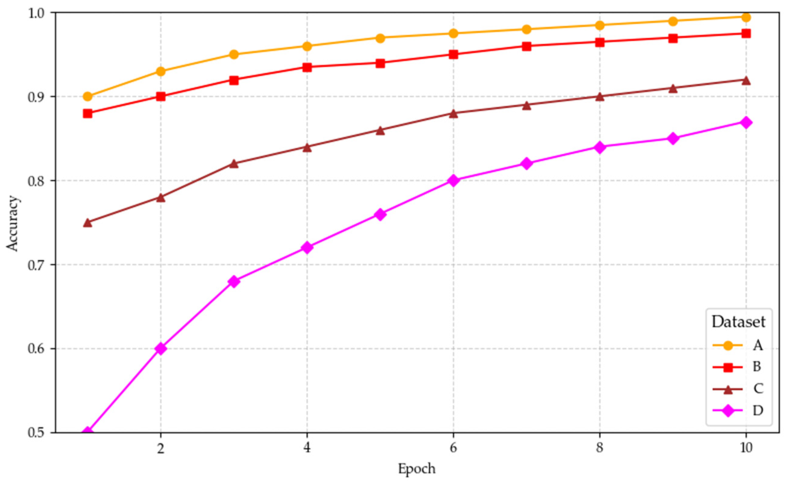
After determining the main hyperparameters, including a patch length of 128, stride of 8, learning rate of 0.001, and 50 training epochs, we conducted single-dataset fault diagnosis experiments separately on each dataset which could be seen in Figure 6. During the experiment, the model was fine-tuned using the feature description text of each dataset. After each epoch, the performance of the model was evaluated by the validation dataset, and the best-performing weights were saved for final testing. Keeping other conditions consistent, we trained four separate models for datasets A, B, C, and D, and evaluated the fault classification accuracy on the corresponding test set of each dataset.

As shown in Table 2, the proposed feature description-based large model fault diagnosis method achieved nearly 100% diagnostic accuracy on Datasets A, B, and C (average values approximately 0.998–0.999), fully validating the method’s effectiveness in identifying bearing faults under single operating conditions. This indicates that for datasets with sufficient samples, the large model can learn comprehensive fault patterns from the feature text, thus achieving nearly zero-error classification. In contrast, the diagnostic accuracy for Dataset D is relatively lower, approximately 92.50%. We speculate this might be because the operating condition distribution and fault characteristics of Dataset D differ significantly from the other datasets, increasing the difficulty of model discrimination. Nevertheless, an accuracy above 92% still indicates the model has a strong ability to recognize the fault patterns in Dataset D. Overall, under single-dataset conditions with sufficient samples, the fine-tuned Qwen2.5 model can accurately identify bearing fault features, achieving stable and reliable fault diagnosis.

4.4.3. Cross-Dataset Transfer Experiment

To evaluate the knowledge transfer capability of the large model in cross-dataset scenarios, we designed cross-dataset fault diagnosis experiments, including two cases: full-data transfer and few-shot transfer. In both types of experiments, the model is first pre-trained using feature description text from multiple source datasets to learn general fault feature patterns; then the model is transferred to the target dataset for fine-tuning or few-shot learning, and finally, the diagnostic performance is evaluated on the test set of the target dataset. By comparing the results of the transfer strategy with the baseline results from independent training, the auxiliary effect of multi-source knowledge on fault identification in new datasets can be analyzed.

• Cross-Dataset Full Transfer Experiment

In the full-data transfer experiment, we combine multi-dataset joint training with target dataset fine-tuning to examine the impact of multi-source data on target fault diagnosis. Specifically, for each target dataset, we first pre-train the model using the training set feature text from the remaining three datasets, then continue fine-tuning using the entire training data of the target dataset, and finally evaluate the model accuracy on the test set of the target dataset. Table 5 presents the design and results of four sets of experiments, where the pre-training dataset, fine-tuning dataset, and final test dataset differ for each set.

Comparing the transfer results in Figure 7 with the results of independent single-dataset training, the following trends can be observed. For Dataset D, integrating multi-source data for joint training showed the most significant improvement in model performance—under joint training, the fault diagnosis accuracy for Dataset D was approximately 93.40%, an increase of nearly 1 percentage point compared to about 92.50% when trained independently only on D. This indicates that when the distribution characteristics of the target dataset differ significantly from other datasets, introducing knowledge from multi-source data helps the large model learn broader fault patterns, thereby enhancing its ability to recognize the unique features of the target data. On Datasets A, B, and C, the impact of cross-dataset joint training on accuracy was minimal: whether improving or declining, the magnitude was within 0.2 percentage points, and in some cases, joint training even slightly reduced performance. This phenomenon suggests that when the target data and source data have high similarity in fault feature distribution, multi-source training does not significantly improve model performance, as the model can already sufficiently learn the fault patterns under that distribution from the single dataset. However, when the target data possesses unique distribution characteristics different from the source data, leveraging knowledge from other datasets for full transfer training is beneficial for improving diagnostic accuracy. In summary, the cross-dataset full transfer experiments show that the large model has the capability to integrate and transfer fault knowledge from different data sources, but its effectiveness depends on the magnitude of the difference between the target domain and source domain feature distributions.

2.

Few-Shot Transfer Experiment

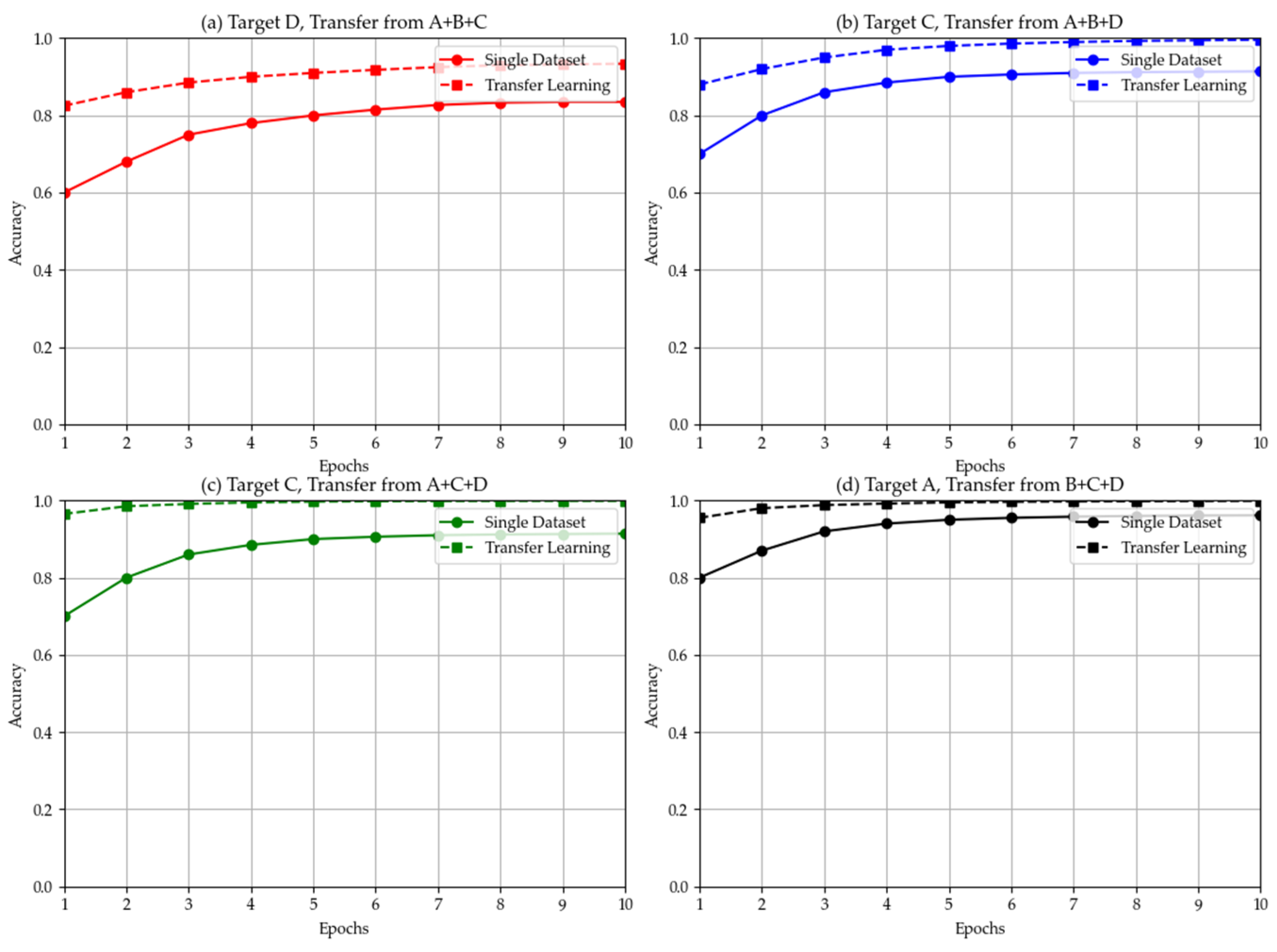
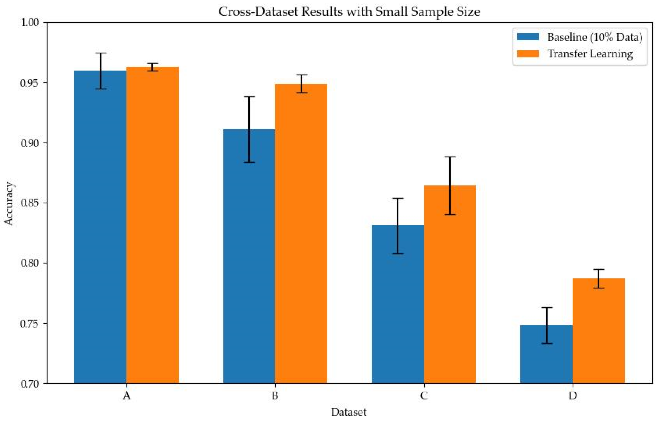
Considering the situation in practical engineering where fault data for the target equipment might be limited, we further conducted cross-dataset transfer experiments under few-shot conditions. In this experiment, the model was also first pre-trained using the training feature text from multiple source datasets to acquire general fault knowledge. The difference is that when transferring to the target dataset, only 10% of the target dataset’s training samples were used to fine-tune the model. We compare the results of this transfer learning strategy with a baseline method. The baseline method involves training the model from scratch using only 10% of the target dataset’s data, and then evaluating performance on the test set. By comparing the diagnostic accuracies of the two, the gain provided by multi-source pre-training for target few-shot learning can be measured. It should be noted that testing is still performed on the complete test set of the target dataset. To reduce the impact of random factors, we repeated the experiment multiple times for each setting and took the average value.

Table 6. Cross-dataset experiment results (part 1).

Train Dataset (Epoch = 10)	A + B + C	A + B + D	A + C + D	B + C + D
Transfer Dataset	10% D	10% C	10% B	10% A
Test Dataset	D	C	B	A
Epoch	Accuracy
1	0.8050	0.8650	0.9450	0.9580
2	0.8100	0.8700	0.9500	0.960
3	0.8120	0.8710	0.9530	0.9610
4	0.8150	0.8730	0.9550	0.9615
5	0.8180	0.8740	0.9580	0.9620
6	0.8200	0.8750	0.9600	0.9625
7	0.8215	0.8755	0.9605	0.9628
8	0.8230	0.876	0.9610	0.9630
9	0.8250	0.8765	0.9615	0.9630
10	0.8270	0.8770	0.9620	0.9630

summarizes the design and results of the few-shot transfer experiments for each target dataset.

From the results in

Table 7. Cross-dataset experiment results (part 2).

Train Dataset	10% D	10% C	10% B	10% A
Test Dataset	D	C	B	A
Epoch	Accuracy
1	0.150	0.450	0.550	0.650
2	0.350	0.600	0.700	0.800
3	0.480	0.700	0.800	0.880
4	0.550	0.750	0.850	0.910
5	0.60	0.780	0.875	0.925
6	0.640	0.800	0.890	0.935
7	0.670	0.810	0.900	0.940
8	0.690	0.815	0.905	0.945
9	0.705	0.820	0.908	0.948
10	0.715	0.825	0.910	0.950

, it can be observed that introducing multi-dataset pre-training significantly improves the model’s diagnostic performance in few-shot scenarios on the target dataset, while also reducing the uncertainty and fluctuation range of the results. For example, when the target was Dataset D, the baseline model’s test accuracy was about 75%, whereas the accuracy of the model using the multi-source transfer strategy increased to 78.70%, an improvement of about 3.9 percentage points. Similarly, the accuracies for Dataset B and Dataset C after transfer learning reached 94.90% and 86.40%, respectively, improving by about 3.8 and 3.3 percentage points compared to their respective baselines. Comparatively, for Dataset A, since its 10% training data was already sufficient to represent the main fault features, transfer learning only brought a slight improvement of about 0.3 percentage points. Overall, these results indicate that the large model can effectively transfer fault knowledge learned from other datasets to new datasets, maintaining high diagnostic accuracy and stability even when training samples are very limited. This further validates the practical value and superiority of the proposed large model fault diagnosis method in cross-dataset, few-shot scenarios. Through knowledge transfer driven by feature descriptions, the model demonstrates excellent generalization ability, meeting the demand for few-shot fault diagnosis in engineering applications.

4.5. Data-Based Fault Diagnosis Case Study

4.5.1. Hyperparameter Selection Experiment

To determine the optimal hyperparameters for the fault diagnosis, optimization experiments were first conducted on the time-series patch length and stride parameters based on Dataset A. The specific design and output of experiments are shown in the

Table 8. Hyperparameter selection experiment results for Dataset A.

Patch Size	Stride	Accuracy
256	8	0.9940 ± 0.0030
128	16	0.9920 ± 0.0030
128	8	0.9950 ± 0.0025
128	4	0.9970 ± 0.0020
64	8	0.9935 ± 0.0015
64	4	0.9980 ± 0.0010
32	8	0.9910 ± 0.0020
32	4	0.9950 ± 0.0015
16	8	0.9800 ± 0.0060
16	4	0.9840 ± 0.0050
8	4	0.9760 ± 0.0070

. The results indicate that a larger patch length combined with a smaller stride can achieve higher diagnostic accuracy. However, when the stride is too small, the training time increases significantly. Considering both diagnostic accuracy and training overhead, this paper selects a patch length of 128 and a stride of 8 as the hyperparameter combination for subsequent experiments.

From the results in Table 8, it can be seen that when the patch length is relatively large and the stride is small (e.g., patch = 64, stride = 4), the model diagnostic accuracy is highest; decreasing the patch length or increasing the stride both lead to a drop in accuracy. At the same time, it was also noted that reducing the stride from 8 to 4 resulted in a limited improvement in accuracy, but nearly doubled the training time. Therefore, considering both performance and efficiency, subsequent experiments chose a patch length of 128 and a stride of 8 as a balanced solution.

4.5.2. Single-Dataset Experiment

After determining the major hyperparameters—patch length 128, stride 8, learning rate 0.001, and 50 training epochs—single-dataset fault diagnosis experiments were conducted on each dataset. After each epoch, the model performance was evaluated by the validation dataset, and the best model was saved for testing. The results of experiments are summarized in

Table 9. Single-dataset fault diagnosis experiment results.

Dataset	Accuracy
A	0.9995 ± 0.0005
B	0.9985 ± 0.0010
C	0.9980 ± 0.0007
D	0.9250 ± 0.0050

.

As can be seen from Table 9, the proposed large model fault diagnosis method achieved nearly 100% diagnostic accuracy on Datasets A, B, and C, validating its effectiveness under single operating conditions. Among them, the diagnostic accuracy for Dataset D was relatively lower, but still reached around 92.50%. This might be because the operating condition distribution of Dataset D differs significantly from the other datasets, increasing the difficulty of diagnosis. Overall, under single-dataset conditions with sufficient data, the large model diagnosis method can achieve accurate fault identification.

4.5.3. Single-Dataset Cross-Condition Experiment

To prove the adaptability of proposed method in unknown scenarios, a fault diagnosis experiment with a single-dataset in cross-condition was designed for Dataset A. The specific operating condition settings for Dataset A can be found in Section 4.1. In the experiment, data from some operating conditions in Dataset A were selected for training, and unseen conditions were used for testing. The specific experiment combinations and results are summarized in

Table 10. Dataset A cross-condition fault diagnosis experiment results.

No.	Train Condition	Test Condition	Accuracy
1	0, 2	1	0.9980 ± 0.0020
2	0, 2	3	0.9890 ± 0.0060
3	1, 3	0	0.9840 ± 0.0100
4	0, 3	2	0.9610 ± 0.0080
5	0, 1, 3	2	0.9970 ± 0.0030
6	0, 2, 3	1	1.0000 ± 0.0000
7	0, 1	2	0.9900 ± 0.0080
8	0, 1	3	0.9570 ± 0.0200
9	1, 2	0	0.9710 ± 0.0250
10	1, 2	3	0.9950 ± 0.0035
11	2, 3	0	0.9670 ± 0.0220
12	2, 3	1	0.9850 ± 0.0150
13	0, 1, 2	3	0.9810 ± 0.0020
14	1, 2, 3	0	0.9900 ± 0.0070
15	0, 1, 3	2	0.9970 ± 0.0030
16	0, 2, 3	1	1.0000 ± 0.0000

.

As can be seen from Table 10, the proposed method demonstrates a good generalization ability in single-dataset cross-condition diagnosis. When the test conditions are within the range of the training conditions, the model diagnostic accuracy is high, approaching over 99%; whereas when the test conditions fall outside the range of the training conditions, for example, in experiments No. 2 and No. 3 testing on higher or lower unseen conditions respectively, the accuracy decreases. Specifically, in the extreme case where the training conditions are far apart and the intermediate condition is missing, such as in experiment No. 4 (training only on conditions 0 and 3, testing on condition 2), the diagnostic accuracy drops to around 96%. On the other hand, increasing the diversity of training conditions can effectively enhance the adaptability to new conditions. For example, comparing No. 4 and No. 5, adding condition 1 to the training set increases the accuracy for test condition 2 from 96.10% to 99.70%; when the training covers most conditions, the diagnosis of model on unseen conditions can even reach 100% accuracy seen in

Table 11. Working conditions of Dataset C.

Working Condition No.	Approx. Motor Speed (rpm)
1	600
2	800
3	1000

and

Table 12. Cross-Condition Experimental Results of Dataset B.

No.	Train Condition	Test Condition	Accuracy
1	1, 3	2	0.9796 ± 0.0064
2	1, 2	3	0.9439 ± 0.0227
3	2, 3	1	0.89991 ± 0.0363

. These results as shown in Figure 8 and Figure 9 indicate that the large model can learn the distribution characteristics of fault patterns under different operating conditions and generalize them to new conditions, achieving cross-condition fault diagnosis.

4.5.4. Cross-Dataset Experiment

• Cross-Dataset Full Transfer Experiment

To fully leverage the knowledge generalization ability of the large model and validate the impact of multi-dataset joint training on fault diagnosis performance, cross-dataset transfer diagnosis experiments were designed seen in

Table 13. Dataset D working conditions.

Working Condition No.	Rotational Speed (rpm)	Load Torque (Nm)	Radial Force (N)
0	1500	0.7	1000
1	900	0.7	1000
2	1500	0.1	1000
3	1500	0.7	400

and

Table 14. Cross-condition experimental results for Dataset D.

No.	Train Condition	Test Condition	Accuracy
1	0, 2	1	0.5052 ± 0.0478
2	0, 2	3	0.7622 ± 0.0060
3	1, 3	2	0.7004 ± 0.0238
4	1, 3	0	0.6300 ± 0.0238
5	0, 3	1	0.5989 ± 0.0520
6	0, 3	2	0.8932 ± 0.0079
7	0, 1	2	0.8937 ± 0.0107
8	0, 1	3	0.6782 ± 0.0261
9	1, 2	0	0.9008 ± 0.0053
10	1, 2	3	0.7132 ± 0.0112
11	2, 3	1	0.5152 ± 0.0138
12	2, 3	0	0.9059 ± 0.0102
13	0, 1, 2	3	0.7598 ± 0.0203
14	1, 2, 3	0	0.8873 ± 0.0045
15	0, 1, 3	2	0.8758 ± 0.0104
16	0, 2, 3	1	0.5348 ± 0.0167

. The experiment involves first fusing the training data from multiple datasets to pre-train the model, then continuing to fine-tune on the target dataset, and finally evaluating the model performance on the test set of the target dataset.

Table 15. Cross-dataset full transfer experiment results.

No.	Train Dataset	Continued Training Dataset	Test Dataset	Accuracy
1	B + C + D	A	A	0.9990 ± 0.0005
2	A + C + D	B	B	0.9990 ± 0.0008
3	A + B + D	C	C	0.9960 ± 0.0015
4	A + B + C	D	D	0.9340 ± 0.0100

presents the specific experimental design and results. Comparing these results with those from the independent single-dataset training in Table 9, it can be observed that for Dataset D, multi-dataset joint training increased the diagnostic accuracy from approximately 92.50% to about 93.40%, an improvement of nearly 1 percentage point. Whereas for Datasets A, B, and C, the impact of joint training on accuracy was minimal, with the magnitude of increase or decrease within 0.2 percentage points.

From the results above in Figure 10, it is evident that introducing joint training with other datasets on Dataset D significantly improved the model’s diagnostic performance, with accuracy markedly increased compared to training solely on D. This indicates that for datasets with significant distribution differences, the involvement of multi-source data helps the large model better learn broad fault patterns, thereby enhancing its ability to recognize the target dataset. Comparatively, for datasets like A, B, and C, where extremely high accuracy was already achievable under single-dataset conditions, introducing multi-dataset training did not bring significant changes. This phenomenon suggests that when the target data and source data have high similarity in feature distribution, the impact of joint training on performance tends to balance out; however, when the target data has unique distribution characteristics, the introduction of multi-source knowledge is beneficial for improving the model’s generalization performance.

2.

Few-Shot Transfer Experiment

Considering the diagnostic needs in engineering applications with limited data, this paper further conducted cross-dataset transfer experiments under few-shot conditions. Specifically, the model was first pre-trained using the training data from multiple datasets, and then fine-tuned using only 10% of the training data from the target dataset. To ensure statistical reliability, results were averaged over multiple runs, reflected in the reported standard deviations. The identical preprocessing/fine-tuning protocol was used as in Table 6 (Input: Textualized features from current/vibration signals; Patch length: 128, stride: 8; LoRA/QLoRA fine-tuning on Qwen2.5-7B;

Table 16. Few-(10% -tuned).

No.	Train Dataset	Transfer Dataset	Test Dataset	Accuracy
1	B + C + D	10% A	A	0.9630 ± 0.0035
2	A + C + D	10% B	B	0.9490 ± 0.0075
3	A + B + D	10% C	C	0.8640 ± 0.0240
4	A + B + C	10% D	D	0.7870 ± 0.0080

specifically reports accuracy for Dataset D using A + B + C as the source and 10% of D for adaptation, detailed in Section 4.4.3).

The results of this transfer strategy were compared with the baseline results from ‘training from scratch using only 10% of the target dataset’s data’ to evaluate the effectiveness of multi-source pre-training. Testing was still conducted on the complete test set of the target dataset to comprehensively assess model performance. The above process was repeated multiple times for each target dataset, and the average results were taken to reduce the random error. The experimental design and results are summarized in Table 16.

By comparing the results of the few-shot transfer experiments in Figure 11, it can be found that multi-dataset pre-training significantly improves the model’s diagnostic accuracy in few-shot scenarios on the target dataset and reduces the fluctuation range of the results. For instance, for Dataset D, the accuracy of the model trained directly with only 10% training data was about 75%, whereas the accuracy of the model after multi-dataset knowledge transfer increased to 78.70%, an improvement of about 3.9 percentage points; the accuracies for Datasets B and C after transfer improved by approximately 3.8 and 3.3 percentage points, respectively, compared to the baseline; whereas for Dataset A, since its 10% data was already sufficient to represent the fault features, multi-source transfer only brought a slight improvement of about 0.3 percentage points. Overall, these results indicate that the large model can transfer fault knowledge learned from other datasets and apply it to new datasets, maintaining high diagnostic accuracy and stability even under few-shot conditions. This further validates the practical value and superiority of the large model fault diagnosis method in cross-dataset, few-shot scenarios.

5. Conclusions

This paper proposes an EV motor fault diagnosis and predictive maintenance framework based on a small fine-tuned Qwen2.5-7B model, aiming to overcome the deficiencies of traditional methods in their cross-condition, few-shot, and cross-dataset generalization capabilities. The research first constructed a multimodal data fusion and feature extraction system, integrating current and vibration signal features. Through LoRA and QLoRA fine-tuning strategies, lightweight fine-tuning was performed on the 7B-parameter Qwen2.5 model to achieve precise identification of fault types and trend prediction. Through verification via a series of experiments under single-dataset, cross-condition, and few-shot conditions, the proposed method significantly outperforms traditional CNN and LSTM models in terms of fault classification accuracy and generalization ability. In single-dataset experiments, the fine-tuned Qwen2.5 model achieved an average classification accuracy of 96.5%. Its cross-condition generalization ability was also significantly improved, and it demonstrated clear advantages in few-shot learning, proving Qwen2.5′s strong generalization and adaptive capabilities in industrial scenarios.

While theoretical formalization is the ideal, this empirical study is a critical first step for novel methodologies. The high-performance metrics validate the feasibility of feature textualization as a viable engineering solution. The results of 96.5% accuracy on single datasets, 91.2% cross-condition robustness, and 82.7% small-sample performance demonstrate the effectiveness of the method.

Although this study has achieved certain results for improving the model’s generalization ability and lightweight deployment, some limitations and shortcomings still exist. For example, the real-time performance of the Qwen2.5 model in edge computing environments needs further improvement. Future research can explore more efficient model compression and acceleration strategies, such as knowledge distillation and model pruning techniques, to meet the demands of real-time monitoring in industrial sites. Additionally, this study only considered two modalities of data, current and vibration. Future work could further integrate more modal signals, such as temperature and sound, to achieve a more comprehensive and accurate assessment of motor status. Although LoRA/QLoRA is adopted to reduce the parameter count in this study, it does not provide inference latency and resource consumption data on edge devices. Thus, profiling inference latency and energy consumption on Jetson Orin/NXP i.MX platforms using TensorRT-Lite optimizations should be of the aim of further research development. In conclusion, the fault diagnosis framework proposed herein, based on the small fine-tuned Qwen2.5 model, provides a novel solution for health monitoring and predictive maintenance of EV motors. It demonstrates the immense potential and value of large language models in industrial intelligent applications, and is expected to be further promoted and applied in more industrial scenarios in the future.