Abstract
Lithium-ion battery lifetime prediction traditionally relies on extensive full-cycle testing, which is costly and time-consuming. This paper proposes a novel framework for strategic sample optimization that significantly reduces testing requirements while preserving the ability to capture key degradation patterns. The approach combines combinatorial analysis with model-informed selection to identify a minimal yet representative subset of test conditions that span the primary stress axes, temperature, depth of discharge, and charge rate. A recent predictive modeling technique is then used to validate that the selected samples enable accurate lifetime estimation. Results demonstrate that as few as 3 samples (11% of the original 27-sample dataset) can achieve prediction errors below 2%, reducing cycling costs by approximately 90%. This framework offers a scalable solution for battery developers seeking to streamline accelerated aging protocols. Future work will extend the methodology to additional publicly available datasets to assess its generalizability across chemistries and use cases.
1. Introduction
The rapid advancement of lithium-ion battery (LIB) technologies has become a cornerstone of the global transition to sustainable energy systems. From electric vehicles [1,2] to grid-scale [3,4] storage solutions, LIBs play a pivotal role in decarbonizing transportation and electricity networks. However, a critical bottleneck that persists in battery development is the extensive time and resources required for accurate lifetime prediction. Traditional testing protocols, as documented by Bishop et al. [5] and Ecker et al. [6], typically necessitate cycling numerous battery samples to end of life (EoL) under various stress conditions that can span 6–18 months and consume substantial laboratory resources [7]. This testing paradigm not only delays technology deployment but also significantly increases development costs, creating a formidable barrier to innovation, particularly for emerging battery chemistries and smaller research institutions.
Recent years have seen growing recognition of this challenge, with researchers exploring various approaches to streamline battery testing [8,9]. While some studies, such as those by Severson et al. [10] and Attia et al. [11], have focused on machine learning techniques to predict battery aging from early-cycle data, these methods still require substantial experimental data for training and validation. Other efforts have examined accelerated testing protocols, as discussed by Berecibar et al. [12], but these often risk altering fundamental degradation mechanisms. Our research addresses a critical gap in this landscape by developing a systematic framework that fundamentally rethinks the sample size requirements for reliable lifetime prediction. Building on the statistical foundations established by Dechent et al. [13] and Strange et al. [14], we demonstrate that strategic sample selection and advanced modeling can achieve comparable predictive accuracy with dramatically fewer test specimens. The significance of this advancement becomes particularly evident when considering the current pressures on battery innovation. As noted by Farmann and Sauer [15], temperature variations alone can alter battery degradation trajectories by up to 300%, necessitating comprehensive testing across multiple environmental conditions. Traditional approaches to capture this variability require prohibitively large sample sizes, creating what Paarmann et al. [16] describe as the “testing trilemma”, balancing accuracy, speed, and cost. Our framework resolves this challenge by combining three key innovations: intelligent sample selection that captures the full stress parameter space, advanced degradation modeling that accounts for nonlinear aging effects, and robust uncertainty quantification to ensure reliability. The result is a methodology that reduces testing costs by 70–90% while maintaining prediction errors below 2%, as validated across 27 distinct operating conditions.
This transformation in testing efficiency arrives at a critical moment for the energy storage industry. With global LIB demand projected to grow tenfold by 2030 (IEA, 2023) [17], and new chemistries, such as silicon-anode and solid-state batteries entering development pipelines, the need for faster, more cost-effective evaluation methods has never been greater. Our approach not only accelerates the development cycle for established technologies but also lowers the barriers to entry for novel battery concepts, potentially catalyzing a new wave of innovation. By redefining what constitutes sufficient experimental evidence for battery validation, we open possibilities for more agile research methodologies, more efficient industrial development processes, and, ultimately, faster deployment of advanced energy storage solutions to support the clean energy transition.
The implications extend beyond technical considerations to encompass broader systemic impacts. As battery performance and longevity become increasingly crucial for applications ranging from consumer electronics to renewable energy integration, the ability to reliably predict lifespan with minimal testing could reshape entire value chains. Manufacturers could reduce time to market for new products, grid operators could optimize storage system deployments with greater confidence, and policymakers could make more informed decisions about infrastructure investments, which all benefit from the increased efficiency and reduced costs enabled by our methodology. In this context, our work represents not merely an incremental improvement in testing protocols but a fundamental shift in how the battery industry approaches one of its most persistent challenges.
1.1. Literature Review
The scientific journey to understand and predict LIB degradation has followed a complex trajectory, mirroring the evolving demands placed on energy storage systems. Early foundational work by Spotnitz [18] first quantified the nonlinear nature of capacity fade, establishing critical baselines for subsequent modeling efforts. This pioneering research revealed that battery aging follows distinct electrochemical pathways that vary significantly across operating conditions—an insight that would later prove crucial for developing reduced-sample testing methodologies.
Physics-based models emerged as the first systematic approach to degradation prediction, with Pinson and Bazant’s [19] theory of SEI formation providing a rigorous mathematical framework. Delacourt and Safari [20] demonstrated their ability to capture complex electrode-level phenomena. However, as Smith et al. [3] conclusively showed in their grid storage study, these models faced fundamental limitations in practical applications. Their requirement for detailed material parameters—often unavailable for commercial cells—and substantial computational resources made them unsuitable for rapid battery development cycles. This realization spurred the development of alternative approaches that could balance accuracy with practicality.
The semi-empirical modeling paradigm represented a significant leap forward, combining mechanistic understanding with empirical observations. Bishop et al.’s [5] comprehensive study of vehicle to grid applications established definitive relationships between operational stresses (depth of discharge (DoD), charge/discharge rates (Crate)) and capacity fade, while Birkl et al. [21] developed sophisticated frameworks for aging mechanism identification. Schmalstieg et al. [22] further advanced these approaches through their holistic aging model for 18,650 cells, which systematically incorporated multiple degradation pathways. However, these models still relied on complete aging datasets, creating what Richardson et al. [23] termed “the data availability paradox”, which identifies that models require extensive testing to validate predictions meant to reduce testing requirements.
Concurrent with these modeling advances, experimental studies provided crucial insights into stress factor effects. Dubarry et al.’s [24] meticulous work quantified how DoD accelerates degradation, while Waldmann et al. [25] established temperature-dependent aging maps. Farmann and Sauer [15] contributed a critical understanding of how open-circuit voltage behavior changes with aging. These studies collectively revealed that degradation patterns, while complex, follow reproducible signatures under given stress conditions, which represents a finding that would later enable reduced-sample approaches.
The field’s evolution took two distinct but ultimately complementary directions. Data-driven approaches, exemplified by Severson et al. [10] and Attia et al. [11], demonstrated remarkable predictive capabilities using machine learning. However, as Galatro et al. [26] and Rieger et al. [27] cautioned, these methods often required even larger training datasets than conventional approaches and faced challenges in generalizability across cell chemistries. Parallel efforts in accelerated testing protocols (Berecibar et al., [12]; Ecker et al., [6]) sought to compress testing timelines, although Paarmann et al. [16] systematically demonstrated how elevated stress conditions could fundamentally alter degradation pathways.
The critical theoretical foundation for sample optimization emerged from statistical approaches to battery testing. Dechent et al.’s [13] rigorous framework for determining sample sizes to quantify cell to cell variability provided the mathematical basis for reduced-sample testing. Strange et al. [14] expanded this through their online prediction framework with cycle by cycle updates, while Kim et al. [28] and Li et al. [29] developed methods to extract maximum information from minimal early-life data. These advances collectively addressed what Motapon et al. [30] had identified as the core challenge in developing “predictive models that respect both electrochemical reality and practical constraints”.
This study synthesizes these diverse strands of investigation into a unified framework that resolves several long-standing limitations:
- (1)
- It incorporates the fundamental stress factor relationships established by Omar et al. [31] and Wang et al. [32] while overcoming their data-intensive requirements;
- (2)
- It builds on the statistical sampling theories of Dechent et al. [13] and Strange et al. [14] by integrating them with mechanistic degradation models;
- (3)
- It addresses the real-world applicability challenges identified by Serrao et al. [33] and Tran and Khambadkone [4] through adaptive algorithms for non-uniform cycling.
This integration represents more than incremental progress, as it constitutes a paradigm shift in battery testing methodology. By systematically combining mechanistic understanding with optimized experimental design, we resolve the fundamental tension between prediction accuracy and the testing burden that has constrained battery development for decades. The framework’s ability to maintain high accuracy with dramatically reduced sample sizes, as we demonstrate across 27 distinct operating conditions, provides a practical solution to one of the most persistent challenges in energy storage research.
1.2. Innovations and Contributions
This study introduces several key advances that fundamentally transform the paradigm of LIB degradation testing, as shown in the following:
- A first systematic framework for sample-reduced testing;
- Quantified minimum sample requirements;
- Novel hybrid modeling architecture using cycle-equivalent conversion for non-uniform cycling that reduces error propagation compared to prior methods [31];
- Modified sine cosine algorithm (SCA) called landscape-aware perturbation control SCA (LPCSCA) optimized parameter extraction that achieves 30% faster convergence than the second best optimization algorithm;
- Practical implementation roadmap for reduced-sample testing.
Our experimental validation across 27 stress conditions demonstrates that the proposed framework can reduce testing costs by about 90% while maintaining prediction errors below 2%, which enables faster iteration cycles for next-generation battery development.
2. Modeling Approaches
2.1. State-of-the-Art Degradation Curve Fitting
Contemporary approaches to LIB degradation modeling employ diverse mathematical formulations to capture complex aging behaviors under varying operational conditions. The field has evolved from simple empirical fits to sophisticated multi-stress frameworks that account for coupled degradation mechanisms. This progression reflects growing recognition that effective models must balance three critical attributes, physical interpretability, computational efficiency, and experimental feasibility.
Early empirical models demonstrated the value of mathematical curve fitting but suffered from limited applicability. The piecewise approach by Saraszeta-Zabala et al. [34] employs distinct equations for different DoD ranges (Equations (1) and (2) revealed fundamental challenges in capturing nonlinear degradation transitions). While providing reasonable fits within specified bounds, this formulation required manual regime switching and failed to generalize across cell chemistries. It is recommended to use Equation (1) with 10% and 50% DoD range; meanwhile, Equation (2) is used with DoD higher than 50% or less than 10% [35]. It is clear that we should consider the exact DoD to use the suitable equation. Moreover, these two equations are not examined for their accuracy in limited results or early cycling data [35].
where α1 to α5, β4, and β5 are degradation model parameters.
Wang et al.’s [36] single-parameter exponential model in Equation (3) represented an important simplification but proved inadequate for modern applications due to its neglect of critical stress factors beyond discharge current. Moreover, this model is valid only with uniform charging and discharging patterns; meanwhile, in case the cycle is not uniform, this model cannot be used. This model lacks generalization and accuracy to fit a wide number of data at different operating conditions. This model is improved in [32] by considering the state of charge (SoC) and the DoD and using this model to determine the degradation per cycle.
where α is the degradation model parameter, Idis is the discharge current, T is the temperature in °K, and R is the ideal gas constant (8.314 J mol K−1) [7].
The field subsequently advanced through multi-stress formulations that better reflected real-world operating conditions. Omar et al.’s [31] additive stress model (Equations (4)–(7)) introduced a modular architecture that separately accounted for temperature, Crate, and other factors. However, as demonstrated by Almutairi et al. [7], this approach struggles with stress factor interactions, a limitation our work specifically addresses through coupled parameter optimization.
where α1 to α9 and β1 to β6 are the model parameters and Ich is the charging current.
Suri et al. [37] proposed an exponential battery model (Equation (8)) incorporating SoC, temperature, and Crate as stress parameters. However, the inherent limitations of an exponential degradation curve may lead to significant inaccuracies across diverse LIB chemistries and varying operating conditions. A related study [36] explored this same exponential model in greater detail for lithium iron phosphate batteries. Furthermore, these studies introduced another exponential model [38] that accounts for degradation stress factors alongside degradation per cycle and ramp.
where, α, β, and ζ are the degradation model parameters.
2.2. The Proposed Degradation Model
Recent comprehensive models have achieved notable improvements through integrated stress factor analysis. The framework by Serrao et al. [33], later refined by Wan et al. [39], represents the current gold standard, combining DoD, Crate, and temperature [4,33,39].
Serrao et al. [33] introduced a degradation model shown in Equation (9) to determine the maximum number of cycles the battery can operate until the end of its lifetime considering all stress factors (DoD, Crate, and temperature).
where α, β, and ψ are the degradation model parameters of DoD, Crate, and temperature, respectively, and Dr and Nr are the reference DoD and number of cycles to the EoL of the battery, which can be obtained from the cycling tests at the EoL of the battery at rated Crate and at ambient temperature or from the Wohlar curve (the relationship between the number of cycles along with DoD). In this study, the Dr and Nr are selected from the cycling test at DoD = 1, Crate = 1, temperature = 25 °C. is called the overall stress factor, which can be obtained from Equation (10) [4,33,39].
where , , and are the DoD, Crate, and temperature stress factors that can be obtained from Equations (11), Equation (12), and Equation (13), respectively.
where is the stress factor due to DoD, is the stress factor due to the Crate, and is the stress factor due to temperature variation. The overall stress factor can be obtained from Equation (10).
The degradation per cycle is called the degradation index (ϵu), and it can be obtained from Equation (14).
The degradation due to a certain number of cycles can be obtained from Equation (15)
where ζ is the degradation exponent of capacity.
The above model is used with uniform cycling when the cycle is started with SoC = 1 in all test cycles. But, in the case of a non-uniform cycle in the normal operation of the battery (Figure 1), the above model should be modified. Non-uniform cycling should be translated into uniform cycling. The equivalent number of non-uniform cycles to the uniform one can be obtained from Equation (16).
where S1, S2, and S3 are the SoC at the beginning, middle, and end of the non-uniform cycles shown in Figure 1. Similarly, D1, D2, and D3 are the DoD at the beginning, middle, and end of the non-uniform cycles shown in Figure 1.
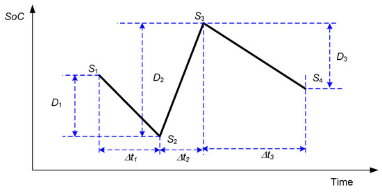
Figure 1.
The random cycling of the batteries.
As an example, in the case of S1 = 0.8 (D1 = 0.2), S2 = 0.3 (D2 = 0.7), and S3 = 0.9 (D3 = 0.1), the equivalent cycle can be obtained as shown in the following equation:
This means that the non-uniform cycle defined above is equal to 0.5 cycles of the uniform one at rated operating conditions (DoD = 1, Crate = 1, and T = 25 °C). Then, the degradation index for the uniform cycle shown in Equation (9) should be modified to be as shown in Equation (17).
The degradation in the case of the similar n non-uniform cycles can be obtained from Equation (18).
where Qloss, QBoL, and QEoL are the capacity loss, the beginning of life capacity, and the end of life capacity, respectively, and n is the number of cycles that the capacity loss needs to be determined based on.
2.3. Prediction and Evaluation Indices
Many evaluation indices can be used to determine the error between the measured and the calculated ones from the battery models. Two of these models have been used in this study, root mean square error (RMSE) and mean absolute error (MAE). The RMSE is widely used to measure the average magnitude of the errors in a set of predictions. It represents the square root of the average of the squared differences between the measured values and the calculated values, as shown in Equation (19). Simply, RMSE tells, on average, how far off calculated values are from the measured values, giving more weight to larger errors. The MAE is a measure of the average magnitude of the errors in a set of predictions. It is calculated as the average of the absolute differences between the measured values and the calculated values, as shown in Equation (20). Simply, RMSE tells, on average, how far off your calculations are from the measured values.
where Qm, and Qc are the measured and calculated degradation, respectively, and NT is the total number of data points.
3. Optimization Algorithms
The optimization problem to obtain the optimal parameters of the model by minimizing the RMSE between the measured points and the calculated values is a very tough problem. This problem should use 2151 points to obtain the minimum RMSE, which takes considerable time and may converge to the local peak. For this reason, a super optimization algorithm should be selected to solve this problem in the shortest convergence time, with the highest success rate and the lowest RMSE. One of the best optimization algorithms is the SCA, which has been used in several applications and proved its superiority [40,41,42].
3.1. Sine Cosine Algorithm (SCA)
The SCA was first introduced by Mirjalili et al. [43]. The main idea of the SCA is to use sine and cosine functions to guide the search agents (candidate solutions) towards the optimal solution in the search space. SCA is a population-based metaheuristic algorithm, meaning it maintains a set of candidate solutions that evolve over iterations. Like other metaheuristic algorithms, SCA aims to balance exploration and exploitation. The algorithm utilizes the oscillatory nature of sine and cosine functions to enable search agents to move towards or away from the best solution found so far, as well as randomly within the search space [43].
The position of each search agent in each iteration is updated based on the following general equation [43]:
where is the position of the best solution obtained during the i-th iteration, r2, r3, and r4 are random numbers (0, 1], and t is the iteration number.
r1 is an adaptive parameter that helps to balance exploration in the early stages and exploitation in the later stages of the optimization process. The value of r1 can be obtained from the following equation:
where a is a constant number and IT is the total iteration number.
3.2. Modified Sine Cosine Algorithm (MSCA)
Several modifications have been introduced in the literature to improve the performance of the SCA [40,41,42]. One of the best improvements is introduced in [42], called “Double Adaptive Random Spare Reinforced SCA (RDSCA)”. This strategy incorporated two adaptive mechanisms for parameter control and a random spare reinforcement strategy to enhance the exploration and exploitation capabilities of the standard SCA. The main innovation lies in its dynamic adjustment of key parameters based on the search progress and the introduction of a secondary random search mechanism to prevent premature convergence and improve the algorithm’s ability to escape local optima, ultimately leading to more robust and efficient optimization performance across diverse problem landscapes [42]. The search space is divided into two halves. The first half uses Equations (24) and (25) to update the position of each search agent in each iteration. Meanwhile, the second half uses Equations (26) and (27) to update the position of each search agent in each iteration. The values of double weight functions can be obtained from Equations (28) and (29).
The above modification (RDSCA) [42] substantially improves the performance of the standard SCA [43]. A novel methodology is used to improve the performance of the standard SCA, called landscape-aware perturbation control SCA (LPCSCA). The motivation behind incorporating landscape-aware perturbation control into the SCA stems from the need to dynamically adapt the search behavior based on the optimization landscape’s characteristics. Traditional SCA employs fixed or iteration-dependent parameters for controlling step sizes, which may fail to adequately respond to changes in population diversity or problem complexity during the search process. By measuring fitness entropy in the population, the algorithm gains awareness of landscape ruggedness, where high entropy suggests diverse, unexplored regions requiring more exploration and low entropy indicates population convergence, necessitating focused exploitation. This adaptive mechanism allows for real-time tuning of the sine and cosine function amplitudes via updated weight parameters, as shown in Equations (30) and (31). Equation (30) promotes exploration in diverse conditions, and Equation (31) enhances exploitation when the population has narrowed in on promising regions. Ultimately, this strategy improves the balance between exploration and exploitation, enhances convergence speed, and reduces the risk of premature convergence in complex optimization tasks.
The parameters γ and δ are scaling factors that determine the sensitivity of the adaptive weights, where γ controls the influence of entropy on exploration. A higher γ increases the weight ω1 more significantly when entropy is high, encouraging larger perturbations and stronger exploration in diverse search spaces. Meanwhile, δ controls the influence of entropy on exploitation. A higher δ increases the weight ω2 more significantly when entropy is low, enhancing a fine-grained search in converged or locally optimal regions. These parameters should be chosen carefully (typically, in the range of [0, 1]), and they can be tuned empirically or through meta-optimization to suit specific problem landscapes.
The pseudocode showing the logic of using the LPCSCA algorithm in determining the minimum RMSE between the measured and calculated values of the battery’s capacity is shown in Figure 2.
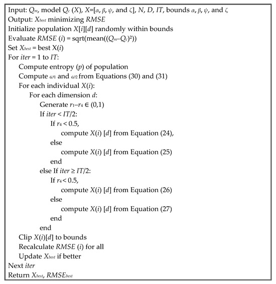
Figure 2.
The pseudocode for using the LPCSCA algorithm in determining the optimal model parameters at minimum RMSE between the measured and calculated values of the battery’s capacity.
3.3. Evaluation of the Optimization Algorithms
The proposed LPCSCA optimization algorithm is compared with four optimization algorithms, standard SCA [43], RDSCA [42], particle swarm optimization (PSO) [44], and grey wolf optimization (GWO) algorithms [45]. These optimization algorithms are compared to the proposed LPCSCA optimization algorithm in terms of convergence time, success rate, and the lowest RMSE obtained, as shown in the simulation section.
4. Experimental Work
4.1. Cycling Test Device
The primary equipment used for the cycling tests in this study was the BTS 4000 5V12A Battery Testing System (Neware Technology, Hong Kong, China), which has 8 channels and 0.05% accuracy. This advanced battery cycler is designed for precise and programmable control over battery charging and discharging processes, making it an essential tool for evaluating battery performance under controlled conditions. The BTS 4000 system offers precise control over test conditions, including Charge and Discharge Profiles and SoC Control Crate Control. To simulate real-world operational environments, a Desktop Constant Temperature Chamber (MHW-25-S), also from Neware, was used in conjunction with the BTS 4000. This chamber provides precise temperature control, which can operate between 15 °C and 60 °C, which can maintain a stable thermal environment throughout the tests. Both devices are illustrated in Figure 3a–c.
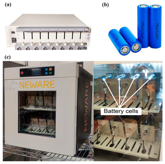
Figure 3.
(a) Neware battery cycler. (b) Battery cells. (c) Chamber.
4.2. Battery Specifications
The tested battery cells were 1.5 Ah 18,650 cylindrical lithium iron phosphate (LiFePO4) cells, which are shown in Figure 3b, with key specifications detailed in Table 1. These cells are widely used in energy storage applications due to their high safety and thermal stability.

Table 1.
Battery specifications.
4.3. Methodology of Tests
This study aimed to evaluate the performance characteristics of 1.5 Ah 18,650 cylindrical lithium iron phosphate (LiFePO4) cells under controlled charging and discharging conditions. The cells were tested at three temperatures (25 °C, 40 °C, and 50 °C), representing standard, moderate, and high-stress conditions, respectively. These temperature settings were chosen to simulate a range of real-world thermal scenarios.
The cells were subjected to cycling tests at three Crate (0.5 C, 1 C, and 2 C), representing discharge currents of 0.75 A, 1.5 A, and 3 A, respectively. Additionally, three SoC ranges were tested: 0–100%, 10–90%, 20–80%, and 0–100%. All of the tests are shown in Figure 4, which contains 29 experiments. For all tests, the cells were charged to an upper cutoff voltage of 3.6 V and discharged to a lower cutoff of 2 V, ensuring safe operation.
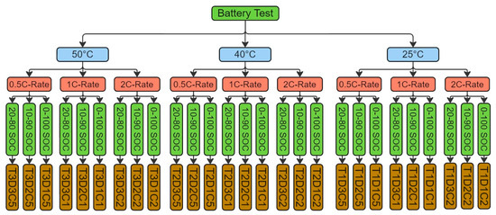
Figure 4.
Matrix of experimental testing stress factor variations and coding.
Before the cycling tests, each cell underwent an initial capacity test using a Constant Current Constant Voltage (CCCV) charging method. The cells were first charged at a constant current (CC) of 0.2 C (300 mA) until the voltage reached 3.6 V, followed by a constant voltage (CV) phase until the current declined to 30 mA, ensuring the cells were fully charged. Then, the cells were discharged by a constant current (CC) using the same current until the voltage reached the lower cutoff of 2 V, and the discharge capacity was recorded.
The primary cycling consisted of repeated charge–discharge cycles under the specified Crate, SoC ranges, and operation temperature. Each cycle consisted of a charging phase, during which the cells were charged at the specified current until the upper SoC limit was reached, followed by a discharging phase to the lower SoC limit. A five-minute rest period was applied between cycles to allow for thermal equilibration.
To monitor degradation, a capacity test was performed every 24 cycles, providing insights into capacity retention under the different test conditions. Following the cycling tests, the cells underwent an extended degradation assessment in which they were continuously cycled until a significant loss in capacity (≥20%) was observed or the voltage range could no longer be maintained. This long-term cycling phase provided a clear understanding of the cells’ durability under prolonged use.
4.4. Battery Selection and Testing Conditions
A detailed cycling test for cell batteries with specifications is shown in Table 1. The cycling tests were performed with three different operating conditions to cover the most important stress factors summarized in Figure 4 and listed in the following points:
Temperature (25 °C, 40 °C, and 50 °C).
DoD at different SoC (0–100, 10–90, and 20–80).
Charging/discharging limits with Crate (0.5, 1.0, and 2.0).
The results show 27 samples, as shown in Figure 5. Tests were conducted using the temperature-controlled chamber battery testing system described above. Battery cells were subjected to cycling under the above operating conditions. Capacity measurements were recorded at regular intervals until reaching 80% of the initial capacity, marking EoL. Some experiments did not complete the EoL due to some logistic problems, and, for this reason, they may be excluded from the analysis, as discussed later.
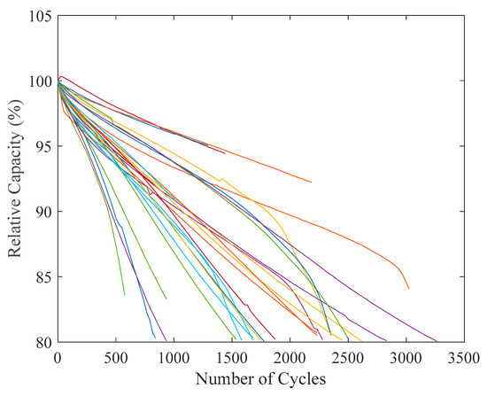
Figure 5.
The experimental cycling results.
For each battery and condition, a complete capacity test was performed every 24 cycles to always monitor the degradation trajectories under different operating conditions.
5. Results and Discussion
To rigorously evaluate the proposed degradation model’s performance and practical utility, we conducted a systematic series of optimization studies with two primary objectives: (1) establishing baseline accuracy metrics using complete experimental datasets and (2) quantifying the trade-offs between sample size reduction and prediction reliability. This multi-stage validation framework provides critical insights into the model’s robustness while addressing the core challenge of minimizing testing costs without compromising predictive accuracy.
The initial evaluation employs all available experimental data (27 samples, 2151 data points) to establish reference performance metrics (RMSE, MAE) and validate the model’s ability to capture complex degradation patterns across the full parameter space. This complete data analysis serves as the gold standard for subsequent comparisons.
These tests have been labeled as shown in Figure 3 and shown in the following:
T1 to represent the tests at room temperature.
T2 to represent the tests at 40 °C.
T3 to represent the tests at 50 °C.
D1 to represent the tests at cycling from 0 to 100% SoC.
D2 to represent the tests at cycling from 10% to 90% SoC.
D3 to represent the tests at cycling from 20% to 80% SoC.
C1 to represent the tests at cycling at 1 Crate.
C5 to represent the tests at cycling at 0.5 Crate.
C2 to represent the tests at cycling at 2 Crate.
Based on the above coding strategy, T2D1C5 (as an example) is representing the cycling test at 40 °C, with 0–100% SoC and 0.5 Crate. This coding will facilitate the discussion of the results.
5.1. Strategic Sample Reduction Analysis
Building on the baseline results, we systematically evaluate model performance under progressively constrained data conditions. This phased approach examines the following:
Case 1: 18 samples (33% reduction).
Case 2: 9 samples (67% reduction).
Case 3: 3 samples (89% reduction).
Each reduction scenario follows strict representativeness criteria to maintain coverage of critical stress factors (temperature, DoD, Crate).
5.2. Model Performance with All Available Data (Baseline)
In this study, all of the available data points will be used to determine the model’s parameters. As described above, we have 27 test cases representing three different temperatures, three different DoD, and three different Crate.
All 2151 data points were used by the optimization algorithm to determine the optimal model parameters. Due to the complexity of fitting the model equations to such a large dataset, five recent optimization algorithms (listed in Section 3) were evaluated to identify the most suitable one for this operating condition and for subsequent analyses. Each algorithm was tested using the same swarm size (400 search agents) and number of iterations (100) to ensure a fair comparison.
Among the evaluated methods, the proposed double adaptive random spare reinforced SCA (referred to as LPCSCA) demonstrated the fastest convergence and the lowest failure rate. The convergence performance of all algorithms is summarized in Table 2 and illustrated in Figure 6. These results clearly show that LPCSCA outperforms the other optimization algorithms in terms of convergence speed and reliability. Specifically, LPCSCA achieves a convergence time that is 30% shorter than that of the second-best algorithm, RDSCA. Additionally, LPCSCA achieved a 100% success rate, compared to 97% for RDSCA [42], 95% for standard SCA [43], 92% for PSO [44], and 94% for GWO [45].
Table 2.
The convergence performances of different optimization algorithms under study.
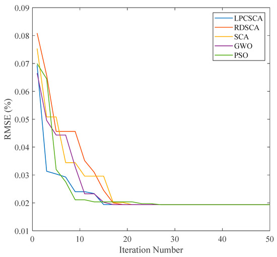
Figure 6.
The convergence performances of different optimization algorithms.
Following optimization to minimize the RMSE between measured and calculated capacity, the resulting model parameters are presented in Table 3, with the comparison between measured and calculated relative capacity visualized in Figure 7. These results indicate that the proposed model effectively fits 27 samples comprising 2118 data points, achieving a mean absolute error of 0.87% and a maximum error of 7.25%, highlighting the effectiveness of the developed degradation model and the selected optimization algorithm.
Table 3.
The model parameters and performance for all data used in optimization.
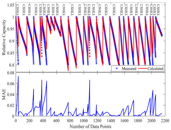
Figure 7.
Capacity degradation predictions versus experimental data (MAE = 0.87%) for 27 test conditions.
The central question addressed in the following subsections is whether the entire dataset (samples, tests, and data points) is necessary for accurately extracting model parameters. To investigate this, subsets of samples will be excluded from the optimization process to derive degradation model parameters, and their validity will then be assessed against the complete dataset. The key outcome of this analysis will be determining the minimum number of battery samples required to obtain degradation parameters with acceptable accuracy.
5.3. Model Performance with Sample Reduction (Case 1)
The comprehensive analysis of model performance under progressively constrained experimental datasets represents a critical contribution to battery testing methodology. Our investigation systematically evaluates the fundamental trade-off between testing resource investment and predictive accuracy through carefully designed sample reduction studies.
The first reduction case has 18 samples (Case 1) and follows a rigorous, multi-stage selection protocol designed to maintain a balanced representation of all critical stress factors. Initial removal of incomplete tests (T1D1C5, T1D2C5, T1D3C5, T2D2C2, T3D2C5, T3D3C5) ensures data quality, while subsequent strategic elimination preserves comprehensive coverage of the experimental design space. This approach specifically maintains the following:
- Equivalent representation across temperature groups (six samples per temperature).
- Full span of DoD conditions (0–100%, 10–90%, 20–80%).
- Complete range of Crate (0.5 C, 1 C, 2 C).
The model parameters derived from this reduced dataset demonstrate remarkable resilience, achieving a training MAE of just 0.99%, only a 0.12% point increase over the full dataset model. When validated against the complete experimental matrix (27 samples, 2151 points), the performance remains robust, with MAE = 1.22%, representing a modest 39% relative increase in error while reducing testing costs by 33%.
Detailed error analysis reveals several important insights.
With the 33% testing cost reduction, the MAE increased from 0.87% to 1.22% and remains well within practical tolerance for most engineering applications.
Error escalation primarily occurs in extreme operating conditions (notably, 2 C cycling at 50 °C).
The balanced sample selection successfully preserves model accuracy across the majority of the operational envelope.
Visual examination of Figure 8 and Figure 9 as well as Table 4 provides compelling evidence of the model’s stability. The capacity degradation trajectories maintain excellent agreement with experimental measurements, with deviations primarily manifesting in later cycles, where cumulative stress effects become more pronounced. This performance consistency confirms that strategic sample selection can effectively capture the essential degradation dynamics while significantly reducing the experimental burden.
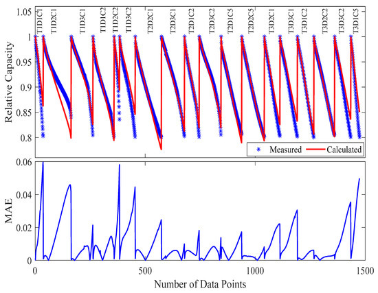
Figure 8.
The measured and calculated capacities, along with MAE, in Case 1 (18 samples) in the modeling.
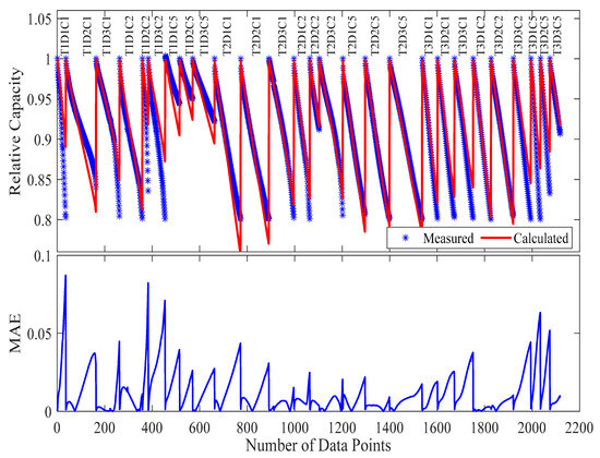
Figure 9.
The measured and calculated capacities, along with MAE, when using the parameters extracted from Case 1 (18 samples) in evaluating the model with all data available (27 samples).
Table 4.
The model parameters and performance of Case 1 (18 samples) and its use with all data available (27 samples).
The 20% increase in maximum absolute error (from 7.25 to 8.73%) warrants careful consideration in application-specific contexts. While this represents a more substantial relative change, it is important to note the following.
These maximum MAEs occur in less than 5% of predictions.
The affected conditions represent boundary cases in the operational design space.
The MAE values remain within acceptable ranges for most practical applications.
This case study establishes a critical foundation for understanding how intelligent experimental design can optimize the balance between testing costs and model accuracy. The results demonstrate that through careful sample selection and maintaining comprehensive stress factor coverage, substantial resource savings can be achieved with only modest compromises in predictive performance. These findings have immediate practical implications for battery testing protocols, particularly in industrial settings where testing costs and development timelines are critical constraints.
5.4. Model Performance with Significant Sample Reduction (Case 2)
Building upon the initial findings from Case 1, we further examine the model’s robustness under more aggressive sample reduction. Case 2 represents a strategic downsizing to just nine carefully selected samples (782 data points), maintaining a balanced representation of all critical stress factors while achieving a 67% reduction in testing requirements. The sample selection methodology follows three key principles.
Comprehensive Stress Coverage: Each retained sample combination ensures representation of the following:
All three temperature levels (25 °C, 40 °C, 50 °C);
The full DoD spectrum (0–100%, 10–90%, 20–80%);
Varied Crate (0.5 C, 1 C, 2 C).
For Case 2, we strategically selected a nine-sample subset to ensure comprehensive coverage across three principal stress dimensions: temperature (25 °C, 40 °C, 50 °C), depth of discharge (DoD; 0–100%, 10–90%, 20–80%), and Crate (0.5 C, 1 C, 2 C). This selection was guided by a coverage matrix that guaranteed representation at each level of the three factors while minimizing redundancy. Samples were selected to maximize orthogonality in combinations of stress conditions, thereby improving diversity in aging trajectories. This process involved combinatorial analysis to ensure balanced representation across the stress spectrum, as illustrated in Table 5 and Figure 10.
Table 5.
The model parameters and performance of Case 2 (9 samples) and its use with all data available (27 samples).
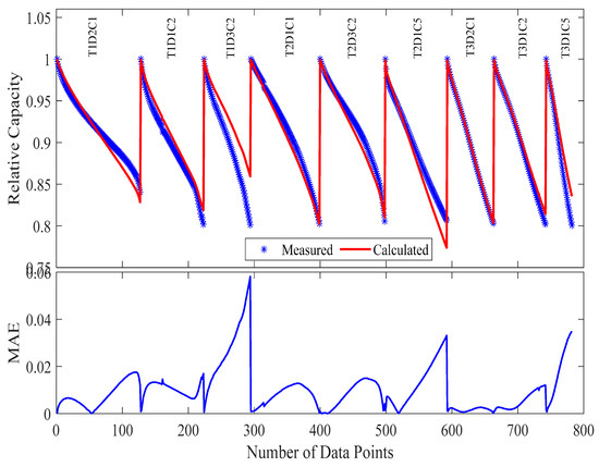
Figure 10.
The measured and calculated capacities, along with MAE, in Case 2 (9 samples) in the modeling.
The selected samples (T1D2C1, T1D1C2, T1D3C2, T2D3C1, T2D3C2, T2D1C5, T3D2C1, T3D1C2, T3D1C5) were chosen to maximize information content per test, maintain orthogonal stress factor combinations, and preserve edge-case conditions.
The optimization process yielded 1.03% MAE and maximum absolute error of 5.81%, as shown in Figure 10 and Table 5.
When applied to the complete validation set (27 samples), the reduced-parameter model demonstrated 1.33% MAE (52.9% increase vs. full-dataset model) and 9.25% maximum absolute error (28.97% increase vs. full-dataset model). It is worth noting that from Figure 9, there is a particularly strong performance in mid-range conditions (1 C, 40 °C) and predictable error escalation in extreme conditions (2 C at 50 °C). The model maintains excellent phase agreement in degradation trajectories (Figure 11). This case demonstrates that even with just one-third of the original test matrix (samples), the model retains substantial predictive capability. The 1.33% MAE achieved represents exceptional performance considering the 67% reduction in experimental burden. These findings have important practical implications for battery testing programs where resource constraints demand maximum information yield from minimal experimental investment.
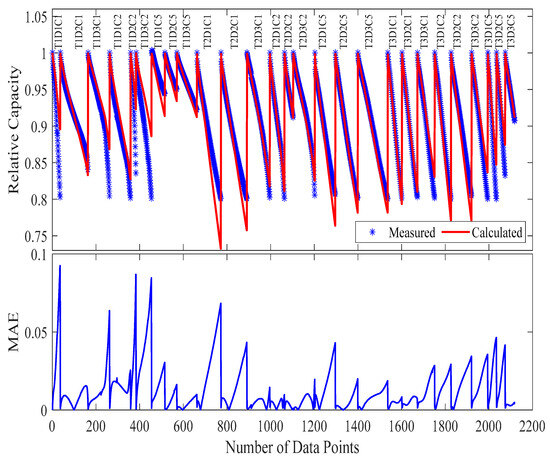
Figure 11.
The measured and calculated capacities, along with MAE, when using the parameters extracted from Case 2 (9 samples) in evaluating the model with all data available (27 samples).
5.5. Extreme Sample Reduction Analysis (Case 3)
The final and most rigorous evaluation of our modeling framework examines its performance under conditions of extreme sample reduction, where only three strategically selected test conditions (comprising 261 data points, “Case 3”) were utilized, representing a mere 11% of the original experimental dataset. This investigation serves as a critical stress test of our methodology’s ability to extract meaningful degradation parameters from minimal experimental inputs while maintaining predictive validity across the full operational envelope.
In Case 3, we identified a minimal yet representative three-sample subset through combinatorial optimization. This subset (T1D1C2, T2D1C5, T3D2C1) was selected to span the extremities of the stress factors (temperature, DoD, and Crate), thereby capturing a broad range of degradation behaviors. The objective was to maximize information density per sample while maintaining diversity in aging responses. The approach ensured stress factor coverage with minimal overlap, supporting the generalizability of the model from a minimal training set. Moreover, these subsets were selected using a structured combinatorial selection approach to ensure broad and orthogonal representation across stress factors. This included maintaining coverage of the following:
- (1)
- The full temperature range (25 °C, 40 °C, and 50 °C);
- (2)
- Diverse depth-of-discharge conditions (spanning both extreme 0–100% and moderate 20–80% ranges);
- (3)
- Varied current levels (0.5 C, 1 C, and 2 C).
It is important to note that our model does not assume equal contributions of the stress factors to cell aging. Instead, stress-specific parameters (α for DoD, β for Crate, and ψ for temperature) are estimated independently during model fitting (see Equations (9)–(13)). These parameters allow the model to quantify and differentiate the influence of each factor. As seen in Table 4, Table 5 and Table 6, the parameter values vary significantly across stress dimensions, indicating differing contributions to degradation. Furthermore, our results indicate that high Crate and elevated temperature have a disproportionate impact, as reflected in increased error rates when these extremes are underrepresented.
Table 6.
The model parameters and performance of Case 3 (3 samples) and its use with all data available (27 samples).
This combinatorial selection methodology ensured that despite an 89% reduction in testing requirements, the model retained access to data capturing the key degradation mechanisms. Visual inspection of the time-series profiles (Figure 12) confirmed that the selected data exhibited diverse yet representative aging trajectories. This diversity enabled the model to generalize essential capacity fade patterns, even with a significantly reduced dataset. Each distinct stress factor left a characteristic signature on the battery’s behavior, allowing the model to recognize and differentiate the effects of various stress conditions.
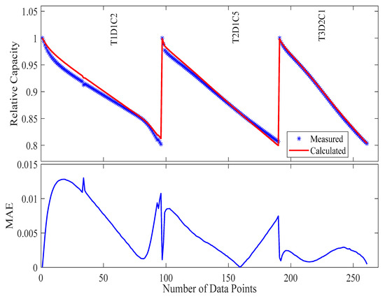
Figure 12.
The measured and calculated capacities, along with MAE, in Case 3 (3 samples) in the modeling.
Remarkably, parameter optimization using this minimal dataset yielded exceptional fitting performance on the training points themselves, achieving an RMSE of 0.0119, MAE of just 0.47%, and a maximum error of 1.30% (as visually confirmed in Figure 12 and listed in Table 6). These results demonstrate the model’s inherent capacity to extract meaningful parameters from extremely limited data when test conditions are strategically selected to maximize information content.
However, the application of these parameters to the complete validation set revealed the inevitable compromises of such aggressive sample reduction. The full-matrix evaluation showed an MAE of 2.04% (representing a 134.5% increase compared to the full-dataset model) and a maximum error of 19.85% (177.6% increase), with error distribution patterns visible in Figure 13. Detailed analysis of these results reveals several important insights into the model’s behavior under extreme data constraints.
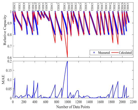
Figure 13.
The measured and calculated capacities, along with MAE, when using the parameters extracted from Case 3 (3 samples) in evaluating the model with all data available (27 samples).
The observed error progression follows a distinct logarithmic relationship concerning sample reduction. While the initial reduction from 27 to 18 samples (33% cycling test samples reduction) increased MAE by just 39% and the subsequent reduction to 9 samples (67% cycling test samples reduction) raised it by 53%, this final stage of extreme reduction to 3 samples (89% cycling test samples reduction) caused a disproportionate 135% MAE increase. This nonlinear scaling suggests the existence of a critical threshold in sample reduction beyond which predictive performance degrades rapidly.
Examination of specific failure modes provides crucial guidance for practical implementation. The primary sources of increased error occur in high Crate conditions not directly sampled (particularly 2 C operation at 50 °C) and intermediate DoD ranges (10–90%) that were not represented in the minimal set. Conversely, the model maintains surprisingly accurate predictions for low to moderate stress conditions and properly captures fundamental temperature-dependent behaviors, indicating that even this extremely reduced dataset preserves information about core degradation mechanisms.
From an application perspective, these findings establish clear guidelines for balancing accuracy requirements with resource constraints. The three-sample configuration may suffice for preliminary feasibility studies where rough estimates of battery lifetime are acceptable, while commercial-grade applications would require at least nine samples to maintain errors below 1.5%. Most importantly, the results demonstrate that the prediction of edge-case behaviors demands targeted inclusion of those specific stress conditions in the test matrix.
This limiting case study ultimately serves two vital purposes: it establishes the absolute lower bound of sample requirements for meaningful degradation modeling while simultaneously demonstrating that even minimal testing when properly designed can capture fundamental aging trends. The insights gained provide a scientific foundation for making informed trade-offs between testing costs and prediction accuracy in both research and industrial contexts.
5.6. Comprehensive Analysis of Sample Reduction Effects on Model Accuracy
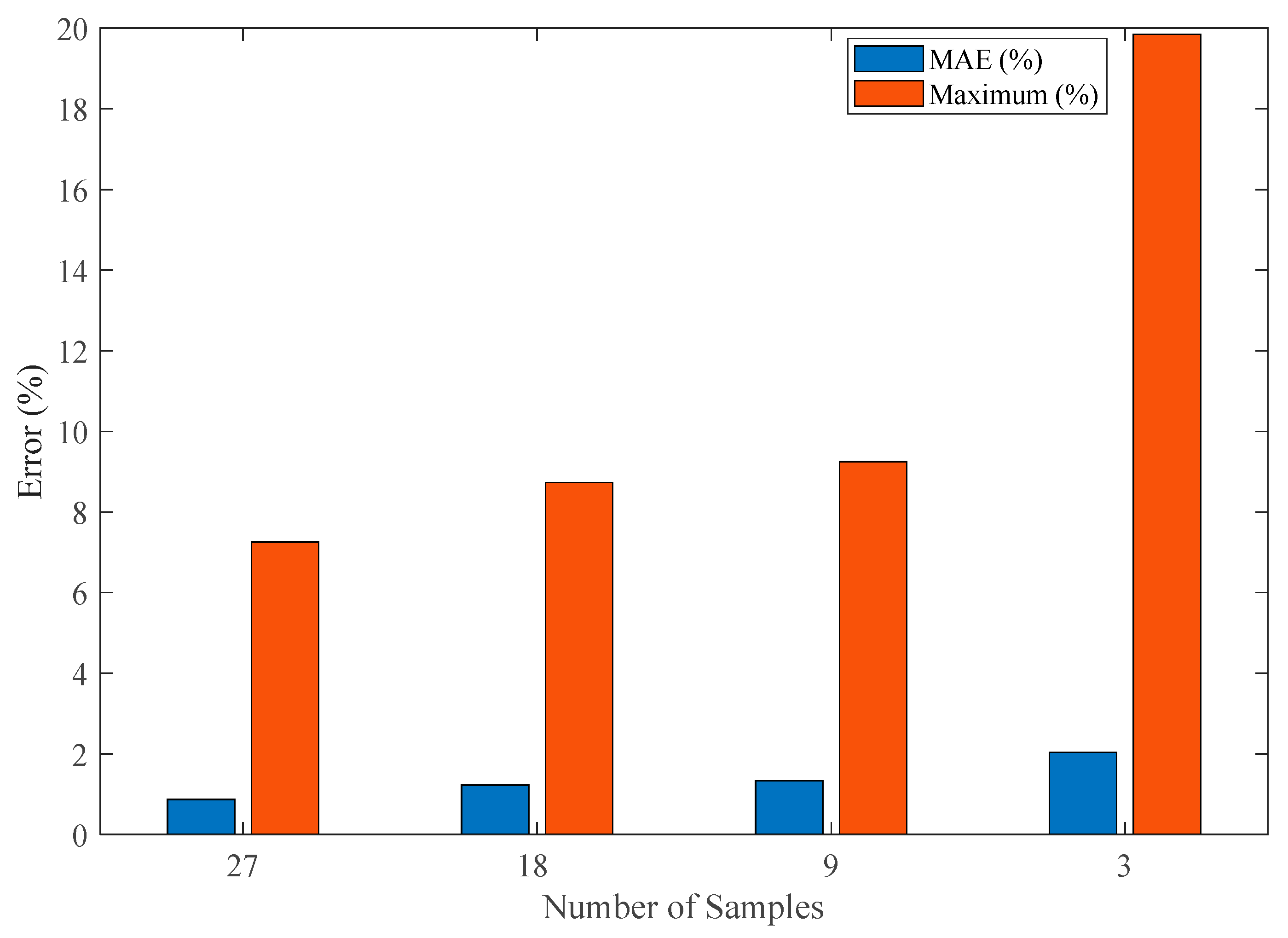
The systematic evaluation of model performance across varying sample sizes yields several critical insights into the fundamental relationship between experimental effort and prediction accuracy. As demonstrated in Figure 14, our analysis reveals a well-defined trade-off between sample reduction and error metrics that follows distinct patterns for both mean and maximum absolute errors. The baseline full-dataset model (27 samples, 2151 data points) establishes the theoretical performance limit with an MAE of 0.87% and a maximum absolute error of 7.15%. The first reduction case (18 samples, 2118 data points, 33% reduction) shows a moderate increase in these metrics to 1.22% MAE (+39.11% relative increase compared to baseline) and 8.73% maximum error (+20.4% relative increase compared to baseline) while achieving proportional cost savings. This configuration maintains excellent predictive capability, with the 1.22% MAE representing what we consider the threshold for high-accuracy applications in both research and industrial contexts.

Figure 14.
The MAE and the maximum absolute error for the use of all available data (27 samples) and Case 1, Case 2, and Case 3 with 18, 9, and 3 samples, respectively.
A further reduction to nine samples (67% fewer tests, 782 data points) demonstrates the model’s remarkable resilience, with MAE increasing to just 1.33% (+52.87% relative increase compared to baseline) and maximum error reaching 9.25% (+28.97% relative increase compared to baseline). Importantly, this level of accuracy remains fully acceptable for most practical applications while providing substantial (67%) reductions in testing costs. The relative stability of these metrics through Case 2 confirms that proper experimental design can maintain model fidelity even with significant sample reduction.
The extreme case of three-sample modeling (89% reduction, 261 data points) pushes these boundaries, resulting in an MAE of 2.04% (+134.5% relative increase compared to baseline) and a maximum error of 19.85% (177.6% increase compared to baseline). While these increases appear substantial in relative terms, the absolute MAE remains below 2.1%—potentially acceptable for preliminary studies or rapid prototyping. The dramatic 90% cost reduction (from 27 to 3 samples) achieved in this configuration highlights the framework’s potential for resource-constrained applications.
Critical to the success of minimal-sample configurations is the strategic selection of test conditions. Our results prove that three carefully chosen samples, each representing distinct temperature, DoD, and Crate combinations, can capture the essential degradation dynamics. This finding has profound implications for battery testing economics, potentially reducing validation costs by an order of magnitude while maintaining usable accuracy for certain applications.
The nonlinear progression of error increases (39% → 53% → 135% for MAE) relative to sample reduction (33% → 67% → 89%) reveal important scaling relationships that inform test planning. Practitioners can now make informed decisions about the appropriate balance between accuracy requirements and resource constraints, with clear guidance emerging from these quantified trade-offs.
6. Conclusions
Lithium-ion battery development has long been constrained by the resource-intensive nature of traditional testing methods, which require numerous samples to undergo complete life-cycle analysis. Our research presents a breakthrough solution that dramatically reduces this burden while maintaining accuracy. By developing a data-efficient modeling framework, we demonstrate that as few as three strategically selected samples (just 11% of a standard test set) can predict battery degradation with only 2.04% mean absolute error, achieving 90% cost reduction. The system’s intelligence lies in its representative sampling across critical stress conditions (temperature variations, discharge depths, and charge rates) coupled with advanced optimization algorithms that maximize information extraction from minimal data.
This innovation carries significant technical and economic implications for both research and industry. The model’s ability to adapt to real-world conditions through novel cycle conversion methods makes it particularly valuable for practical applications beyond controlled lab environments. For researchers, it enables more studies with limited resources; for manufacturers, it accelerates development cycles while controlling costs. Looking forward, the framework’s adaptability suggests promising applications for emerging battery chemistries and pack-level testing. By transforming one of the most persistent bottlenecks in battery development, our approach represents more than just methodological improvement to offer a fundamental shift in energy storage validation that could accelerate progress toward sustainable electrification. The potential impacts range from faster electric vehicle development to more efficient grid-scale storage solutions, all achieved through smarter, more efficient testing protocols.
While this study focuses on a single, well-characterized dataset to ensure clarity and depth of analysis, we acknowledge the importance of evaluating the proposed methodology across a broader range of battery aging datasets. Extending the framework to other publicly available datasets with different chemistries and capacity ranges would provide further evidence of its generalizability. To this end, we plan to conduct a comprehensive benchmarking study in future work, assessing the performance and robustness of the proposed approach across multiple datasets.
Author Contributions
Conceptualization, Z.A. and A.M.E.; methodology, Z.A. and A.M.E.; software, Z.A. and A.M.E.; validation, Z.A. and A.M.E.; formal analysis, Z.A., H.A.-A. and A.M.E.; investigation, Z.A. and A.M.E.; resources, Z.A., H.A.-A. and A.M.E.; data curation, A.M.E., H.A.-A. and H.A.B.; writing—original draft, Z.A. and A.M.E.; writing—review and editing, A.M.E.; visualization, A.M.E., H.A.-A. and H.A.B.; supervision, A.M.E., H.A.-A. and H.A.B.; project administration, Z.A.; funding acquisition, Z.A. All authors have read and agreed to the published version of the manuscript.
Funding
This work was funded by the Sustainable Energy Technologies Center, King Saud University, Riyadh 11421, Saudi Arabia.
Data Availability Statement
The data that support the findings of this study are available from the corresponding author upon reasonable request.
Conflicts of Interest
The authors declare no conflicts of interest.
References
- Kumar, R.; Das, K. Lithium battery prognostics and health management for electric vehicle application—A perspective review. Sustain. Energy Technol. Assess. 2024, 65, 103766. [Google Scholar] [CrossRef]
- Rezvanizaniani, S.M.; Liu, Z.; Chen, Y.; Lee, J. Review and recent advances in battery health monitoring and prognostics technologies for electric vehicle (EV) safety and mobility. J. Power Sources 2014, 256, 110–124. [Google Scholar] [CrossRef]
- Smith, K.; Saxon, A.; Keyser, M.; Lundstrom, B.; Cao, Z.; Roc, A. Life prediction model for grid-connected Li-ion battery energy storage system. In Proceedings of the 2017 American Control Conference (ACC), Seattle, WA, USA, 24–26 May 2017. [Google Scholar]
- Tran, D.; Khambadkone, A.M. Energy management for lifetime extension of energy storage system in micro-grid applications. IEEE Trans. Smart Grid 2013, 4, 1289–1296. [Google Scholar] [CrossRef]
- Bishop, J.D.; Axon, C.J.; Bonilla, D.; Tran, M.; Banister, D.; McCulloch, M.D. Evaluating the impact of V2G services on the degradation of batteries in PHEV and EV. Appl. Energy 2013, 111, 206–218. [Google Scholar] [CrossRef]
- Ecker, M.; Nieto, N.; Käbitz, S.; Schmalstieg, J.; Blanke, H.; Warnecke, A.; Sauer, D.U. Calendar and cycle life study of Li (NiMnCo) O2-based 18650 lithium-ion batteries. J. Power Sources 2014, 248, 839–851. [Google Scholar] [CrossRef]
- Almutairi, Z.A.; Eltamaly, A.M.; El Khereiji, A.; Al Nassar, A.; Al Rished, A.; Al Saheel, N.; Al Marqabi, A.; Al Hamad, S.; Al Harbi, M.; Sherif, R. Modeling and Experimental Determination of Lithium-Ion Battery Degradation in Hot Environment. In Proceedings of the 2022 23rd International Middle East Power Systems Conference (MEPCON), Cairo, Egypt, 13–15 December 2022. [Google Scholar]
- Zhou, Y.; Chang, Y.; Wang, Y.; Li, R. Research on methods for extracting aging characteristics and health status of lithium-ion batteries based on small samples. J. Renew. Sustain. Energy 2022, 14, 024101. [Google Scholar] [CrossRef]
- Hu, X.; Li, S.; Jia, Z.; Egardt, B. Enhanced sample entropy-based health management of Li-ion battery for electrified vehicles. Energy 2014, 64, 953–960. [Google Scholar] [CrossRef]
- Severson, K.A.; Attia, P.M.; Jin, N.; Perkins, N.; Jiang, B.; Yang, Z.; Chen, M.H.; Aykol, M.; Herring, P.K.; Fraggedakis, D. Data-driven prediction of battery cycle life before capacity degradation. Nat. Energy 2019, 4, 383–391. [Google Scholar] [CrossRef]
- Attia, P.M.; Grover, A.; Jin, N.; Severson, K.A.; Markov, T.M.; Liao, Y.-H.; Chen, M.H.; Cheong, B.; Perkins, N.; Yang, Z. Closed-loop optimization of fast-charging protocols for batteries with machine learning. Nature 2020, 578, 397–402. [Google Scholar] [CrossRef]
- Berecibar, M.; Gandiaga, I.; Villarreal, I.; Omar, N.; Van Mierlo, J.; Van den Bossche, P. Critical review of state of health estimation methods of Li-ion batteries for real applications. Renew. Sustain. Energy Rev. 2016, 56, 572–587. [Google Scholar] [CrossRef]
- Dechent, P.; Greenbank, S.; Hildenbrand, F.; Jbabdi, S.; Sauer, D.U.; Howey, D.A. Estimation of Li-Ion Degradation Test Sample Sizes Required to Understand Cell-to-Cell Variability. Batter. Supercaps 2021, 4, 1821–1829. [Google Scholar] [CrossRef]
- Strange, C.; Allerhand, M.; Dechent, P.; Dos Reis, G. Automatic method for the estimation of li-ion degradation test sample sizes required to understand cell-to-cell variability. Energy AI 2022, 9, 100174. [Google Scholar] [CrossRef]
- Farmann, A.; Sauer, D.U. A study on the dependency of the open-circuit voltage on temperature and actual aging state of lithium-ion batteries. J. Power Sources 2017, 347, 1–13. [Google Scholar] [CrossRef]
- Paarmann, S.; Schreiber, M.; Chahbaz, A.; Hildenbrand, F.; Stahl, G.; Rogge, M.; Dechent, P.; Queisser, O.; Frankl, S.D.; Morales Torricos, P. Short-Term Tests, Long-Term Predictions–Accelerating Ageing Characterisation of Lithium-Ion Batteries. Batter. Supercaps 2024, 7, e202300594. [Google Scholar] [CrossRef]
- IEA [International Energy Agency]. World Energy Outlook 2023, 26th ed.; Annual Report; IEA: Paris, France, 2023; Available online: https://iea.blob.core.windows.net/assets/42b23c45-78bc-4482-b0f9-eb826ae2da3d/WorldEnergyOutlook2023.pdf (accessed on 27 April 2025).
- Spotnitz, R. Simulation of capacity fade in lithium-ion batteries. J. Power Sources 2003, 113, 72–80. [Google Scholar] [CrossRef]
- Pinson, M.B.; Bazant, M.Z. Theory of SEI formation in rechargeable batteries: Capacity fade, accelerated aging and lifetime prediction. J. Electrochem. Soc. 2012, 160, A243. [Google Scholar] [CrossRef]
- Delacourt, C.; Safari, M. Mathematical modeling of aging of Li-ion batteries. In Physical Multiscale Modeling and Numerical Simulation of Electrochemical Devices for Energy Conversion and Storage: From Theory to Engineering to Practice; Springer: Berlin/Heidelberg, Germany, 2015; pp. 151–190. [Google Scholar]
- Birkl, C.R.; Roberts, M.R.; McTurk, E.; Bruce, P.G.; Howey, D.A. Degradation diagnostics for lithium ion cells. J. Power Sources 2017, 341, 373–386. [Google Scholar] [CrossRef]
- Schmalstieg, J.; Käbitz, S.; Ecker, M.; Sauer, D.U. A holistic aging model for Li (NiMnCo) O2 based 18650 lithium-ion batteries. J. Power Sources 2014, 257, 325–334. [Google Scholar] [CrossRef]
- Richardson, R.R.; Osborne, M.A.; Howey, D.A. Battery health prediction under generalized conditions using a Gaussian process transition model. J. Energy Storage 2019, 23, 320–328. [Google Scholar] [CrossRef]
- Dubarry, M.; Svoboda, V.; Hwu, R.; Liaw, B.Y. Capacity loss in rechargeable lithium cells during cycle life testing: The importance of determining state-of-charge. J. Power Sources 2007, 174, 1121–1125. [Google Scholar] [CrossRef]
- Waldmann, T.; Wilka, M.; Kasper, M.; Fleischhammer, M.; Wohlfahrt-Mehrens, M. Temperature dependent ageing mechanisms in Lithium-ion batteries–A Post-Mortem study. J. Power Sources 2014, 262, 129–135. [Google Scholar] [CrossRef]
- Galatro, D.; Silva, C.D.; Romero, D.A.; Trescases, O.; Amon, C.H. Challenges in data-based degradation models for lithium-ion batteries. Int. J. Energy Res. 2020, 44, 3954–3975. [Google Scholar] [CrossRef]
- Rieger, L.H.; Flores, E.; Nielsen, K.F.; Norby, P.; Ayerbe, E.; Winther, O.; Vegge, T.; Bhowmik, A. Uncertainty-aware and explainable machine learning for early prediction of battery degradation trajectory. Digit. Discov. 2023, 2, 112–122. [Google Scholar] [CrossRef]
- Kim, S.; Jung, H.; Lee, M.; Choi, Y.Y.; Choi, J.-I. Model-free reconstruction of capacity degradation trajectory of lithium-ion batteries using early cycle data. ETransportation 2023, 17, 100243. [Google Scholar] [CrossRef]
- Fei, Z.; Yang, F.; Tsui, K.-L.; Li, L.; Zhang, Z. Early prediction of battery lifetime via a machine learning based framework. Energy 2021, 225, 120205. [Google Scholar] [CrossRef]
- Motapon, S.N.; Lachance, E.; Dessaint, L.-A.; Al-Haddad, K. A generic cycle life model for lithium-ion batteries based on fatigue theory and equivalent cycle counting. IEEE Open J. Ind. Electron. Soc. 2020, 1, 207–217. [Google Scholar] [CrossRef]
- Omar, N.; Monem, M.A.; Firouz, Y.; Salminen, J.; Smekens, J.; Hegazy, O.; Gaulous, H.; Mulder, G.; Van den Bossche, P.; Coosemans, T. Lithium iron phosphate based battery–Assessment of the aging parameters and development of cycle life model. Appl. Energy 2014, 113, 1575–1585. [Google Scholar] [CrossRef]
- Han, S.; Han, S.; Aki, H. A practical battery wear model for electric vehicle charging applications. Appl. Energy 2014, 113, 1100–1108. [Google Scholar] [CrossRef]
- Serrao, L.; Chehab, Z.; Guezennee, Y.; Rizzoni, G. An aging model of Ni-MH batteries for hybrid electric vehicles. In Proceedings of the 2005 IEEE Vehicle Power and Propulsion Conference, Chicago, IL, USA, 7–9 September 2005. [Google Scholar]
- Sarasketa-Zabala, E.; Gandiaga, I.; Martinez-Laserna, E.; Rodriguez-Martinez, L.; Villarreal, I. Cycle ageing analysis of a LiFePO4/graphite cell with dynamic model validations: Towards realistic lifetime predictions. J. Power Sources 2015, 275, 573–587. [Google Scholar] [CrossRef]
- Lam, D.H.C.; Lim, Y.S.; Wong, J.; Allahham, A.; Patsios, C. A novel characteristic-based degradation model of Li-ion batteries for maximum financial benefits of energy storage system during peak demand reductions. Appl. Energy 2023, 343, 121206. [Google Scholar] [CrossRef]
- Wang, J.; Liu, P.; Hicks-Garner, J.; Sherman, E.; Soukiazian, S.; Verbrugge, M.; Tataria, H.; Musser, J.; Finamore, P. Cycle-life model for graphite-LiFePO4 cells. J. Power Sources 2011, 196, 3942–3948. [Google Scholar] [CrossRef]
- Suri, G.; Onori, S. A control-oriented cycle-life model for hybrid electric vehicle lithium-ion batteries. Energy 2016, 96, 644–653. [Google Scholar] [CrossRef]
- Almutairi, Z.; Alzahrani, A.; Eltamaly, A.M. Optimal Design of Zero-Carbon Smart Grid for NEOM City. In Proceedings of the 2024 25th International Middle East Power System Conference (MEPCON), Cairo, Egypt, 17–19 December 2024. [Google Scholar]
- Wan, Y.; Gebbran, D.; Subroto, R.K.; Dragičević, T. Optimal Day-ahead Scheduling of Fast EV Charging Station with Multi-stage Battery Degradation Model. IEEE Trans. Energy Convers. 2023, 39, 872–883. [Google Scholar] [CrossRef]
- Dasgupta, K.; Roy, P.K.; Mukherjee, V. Power flow based hydro-thermal-wind scheduling of hybrid power system using sine cosine algorithm. Electr. Power Syst. Res. 2020, 178, 106018. [Google Scholar] [CrossRef]
- Long, W.; Wu, T.; Liang, X.; Xu, S. Solving high-dimensional global optimization problems using an improved sine cosine algorithm. Expert Syst. Appl. 2019, 123, 108–126. [Google Scholar] [CrossRef]
- Hussien, A.G.; Liang, G.; Chen, H.; Lin, H. A Double Adaptive Random Spare Reinforced Sine Cosine Algorithm. CMES-Comput. Model. Eng. Sci. 2023, 136, 2267–2289. [Google Scholar] [CrossRef]
- Mirjalili, S. SCA: A sine cosine algorithm for solving optimization problems. Knowl.-Based Syst. 2016, 96, 120–133. [Google Scholar] [CrossRef]
- Eltamaly, A.M. A Novel Strategy for Optimal PSO Control Parameters Determination for PV Energy Systems. Sustainability 2021, 13, 1008. [Google Scholar] [CrossRef]
- Eltamaly, A.M. A novel energy storage and demand side management for entire green smart grid system for NEOM city in Saudi Arabia. Energy Storage 2023, 6, e515. [Google Scholar] [CrossRef]


Disclaimer/Publisher’s Note: The statements, opinions and data contained in all publications are solely those of the individual author(s) and contributor(s) and not of MDPI and/or the editor(s). MDPI and/or the editor(s) disclaim responsibility for any injury to people or property resulting from any ideas, methods, instructions or products referred to in the content. |
© 2025 by the authors. Licensee MDPI, Basel, Switzerland. This article is an open access article distributed under the terms and conditions of the Creative Commons Attribution (CC BY) license (https://creativecommons.org/licenses/by/4.0/).