Abstract
With the large-scale integration of wind power, transient stability issues in power systems have become increasingly prominent, among which the impact of the active power recovery rate of wind turbines on system stability cannot be ignored. This paper establishes a sensitivity analytical model between the transient stability index of the system and the active power recovery rate of doubly fed induction generators (DFIGs), revealing the influence of active power recovery rate on system stability. First, the trajectory analysis method is adopted as the transient stability assessment approach, proposing a stability index incorporating accelerating power and transient potential energy. Analytical sensitivity models for synchronous generator accelerating power and transient potential energy to the active power recovery rate of wind turbines are derived in a simplified system. Second, a sensitivity model of the stability margin index to the active power recovery rate is constructed to analyze the influence patterns of the active power recovery rate, initial active power output of wind turbines, and fault duration time on system stability. This research demonstrates that: accelerating the active power recovery rate can restore power balance more quickly but it reduces the rate of transient potential energy variation and delays the peak response of potential energy, thereby decreasing the stability margin; higher initial active power output of wind turbines suppresses the oscillation amplitude of synchronous generators but increases the risk of power imbalance; and prolonged fault duration exacerbates transient energy accumulation and significantly degrades system stability. Additionally, for each 0.1 p.u./s increase in the active power recovery rate of the wind turbine, the absolute value of the stability index of the synchronous machine in the single-machine system decreases by approximately 0.5–1.0, while the sensitivity decreases by approximately 0.01–0.02 s−1. In the multi-machine system, the absolute value of the stability index of the critical machine decreases by approximately 5–10, and the sensitivity decreases by approximately 0.5–1.0 s−1.
1. Introduction
Transient stability is an important part of power system safety and stability analysis. With the large-scale integration of wind power into the grid, the dynamic characteristics of wind turbines have a significant impact on the transient stability of the power system, which brings new challenges to the traditional power system [1,2]. Different from synchronous units, wind turbines have fast and adjustable active recovery characteristics, and this dynamic response difference will change the energy balance relationship in the transient process of the system and affect the rotor motion characteristics and transient stability margin of the synchronous unit. Therefore, it is of great significance to reveal the mechanism of the active power recovery rate and the transient stability margin of the wind turbine to ensure the stable operation of the new power system.
At present, a large number of studies have explored the impact of wind turbines on the stability of the power system. The numerical simulation method [3] solves the differential algebraic equations before and after the system is disturbed by the numerical integration algorithm and then judges whether the system is stable according to the numerical solution. Refs. [4,5] analyze the effects of different models, capacities, and permeability of wind turbines on the power angle stability of the synchronous turbine and point out that the active power output of the synchronous turbine and the inertia level of its critical group play a major role in the transient stability margin of the system. A nonlinear order reduction model of multiple wind turbines based on phase-locked loops was established in Ref. [6] to reveal the relationship between the position of the units in the wind farm and their transient stability, as well as the interaction between the stability of the wind farms, indicating that the units with large active power output will be more prone to instability for the units on the same low-voltage feeder. It is pointed out in Refs. [7,8] that the reactive power support strategy of wind turbines has an important impact on the stability of the power system. In the system, the influence of the wind turbine on the transient stability of the system under different fault locations is studied [9]. Although the numerical simulation method can be used to study the influence of wind turbines on the stability of the power system, it is difficult to give a mechanism explanation of the influence of wind turbines on the transient stability of the system, and it is impossible to quantitatively evaluate the stability of the system.
The direct method [10] is a stability analysis method based on the energy of the system law. In Refs. [11,12], the power angle stability is theoretically analyzed based on the equivalent external characteristics of doubly fed wind turbines during failure and the power characteristic equation of single-ended transmission systems. Based on the electromagnetic power equation of the synchronous machine, the influence of wind power output substitution for thermal power on the initial power angle of the synchronous machine was studied and the influence of DFIG access on the stability of the transient power angle was analyzed by the equal area rule [13]. After analyzing the dynamic characteristics of doubly fed wind turbines, Refs. [14,15] pointed out that under certain conditions the dynamic model can be simplified to a power injection model, and a criterion for evaluating the influence of wind power access on the transient stability of the system was proposed. According to the energy function of the stochastic network, a mathematical model of power system based on stochastic perturbation was proposed in Ref. [16], and the influence of the intensity and type of stochastic perturbation on the transient stability of the power system was studied. In Ref. [17], a method was proposed to analyze the influence of the wind power access ratio on the transient power angle stability of power system, and the equivalent rotor motion equation with the wind power ratio was constructed to quantify the influence of the wind power access ratio on system stability. Ref. [18] derives a transient energy function for permanent magnet synchronous generator (PMSG)-based wind farms considering inertial control and outer-loop control effects. This enables rapid and effective assessment of the system’s transient stability. Ref. [19] through comparative analysis of two scenarios—direct grid integration of wind power and equivalent-capacity replacement of synchronous generators—investigated the impact of centralized DFIG-based wind power integration on power system transient rotor angle stability. The existing research mainly focuses on the mechanism of the control strategy on the transient stability of the wind turbine during fault ride-through, but there is still a lack of systematic research on the influence of the dynamic recovery process of the active power of the wind turbine on the transient stability of the system after the fault is cleared.
In the technical specifications for wind farm integration into power systems, to ensure grid stability, wind turbines are generally required to possess low-voltage ride-through (LVRT) control capabilities during power system faults. Among these, active power recovery control for wind turbines constitutes a critical component of LVRT control. Its primary function is to gradually restore the active power of wind turbines to pre-fault levels at a predetermined recovery rate after fault clearance, playing a vital role in the transient stability of power systems [20]. However, the systematic analysis of the influence of the active recovery rate of wind turbines on the transient stability of the system is still insufficient in the existing studies. Ref. [21] constructs an equivalent single-machine infinite-bus (SMIB) system model suitable for analyzing transient rotor angle stability in wind-integrated systems. It reveals the mechanism by which post-fault active power control of DFIG-based wind farms influences the first two swing instabilities of transient rotor angles. Ref. [22] pointed out that the fault response characteristics of doubly fed wind turbines depend on their ride-through control strategies, but in the fault clearing stage, the active power recovery control link of wind turbines has little influence on the power angle stability of the system. Ref. [23] addresses the impact of time-varying voltage, current, and power characteristics of DFIGs after fault clearance on the first-swing rotor angle stability of wind–thermal bundled systems. It establishes a time-varying impedance model incorporating DFIG dynamic characteristics. By applying the equal area criterion, the study analyzes the influence of active power recovery rates on the first-swing amplitude under varying conditions, uncovering the impact patterns of active power recovery rates on first-swing stability across different system parameters. Ref. [24] employs a power injection model to describe DFIGs and explores the effects of wind turbine integration on system transient stability under different active power recovery rates during fault recovery, along with corresponding stability criteria. In the above study, it is difficult to directly quantify the relationship between the recovery rate and the stability margin when analyzing the influence of the power recovery rate after the fault ride through of doubly fed wind turbines on the transient stability of the system, and there is a lack of quantitative characterization and mechanism explanation of the relationship between the active recovery rate of wind turbines and the transient stability margin of the system.
In summary, research on the impacts of wind power integration on power system transient stability has primarily focused on the dynamic response characteristics of wind turbines during faults, while insufficient systematic analysis has been conducted on the active power recovery process after fault clearance. Among existing methods, numerical simulation can reveal phenomena patterns but lacks mechanistic explanations and quantitative evaluations; the direct method based on energy function theory can quantify the relationship between wind power penetration and stability margin, yet struggles to characterize the coupling effects of time-varying parameters (e.g., active power recovery rate) on dynamic processes. The research bottleneck lies in the following areas: (1) the quantitative correlation mechanism between post-fault active power recovery dynamics and system stability margin remaining unclear, and (2) the absence of quantitative analysis on the relationship between wind turbine dynamic power recovery characteristics and system transient stability margin. To address this, this paper proposes the following novel trajectory analysis-based framework: by constructing sensitivity models of a synchronous machine accelerating power and potential energy to wind turbine active power recovery rate, a direct quantitative mapping relationship between “wind turbine active power recovery rate—stability index [25]” is established. Subsequently, the impacts of variations in wind turbine active power recovery rate on system stability are analyzed, with validation of the proposed models and patterns in both single-machine and multi-machine systems. This method circumvents the limitations of traditional energy functions in modeling time-varying dynamics, enables precise analysis of the time-domain mechanisms through which active power recovery rate, initial power, and fault duration affect transient energy accumulation, and verifies model effectiveness through multi-scenario simulations, providing theoretical support for adaptive control of high-renewable-penetration power systems.
2. Materials and Methods
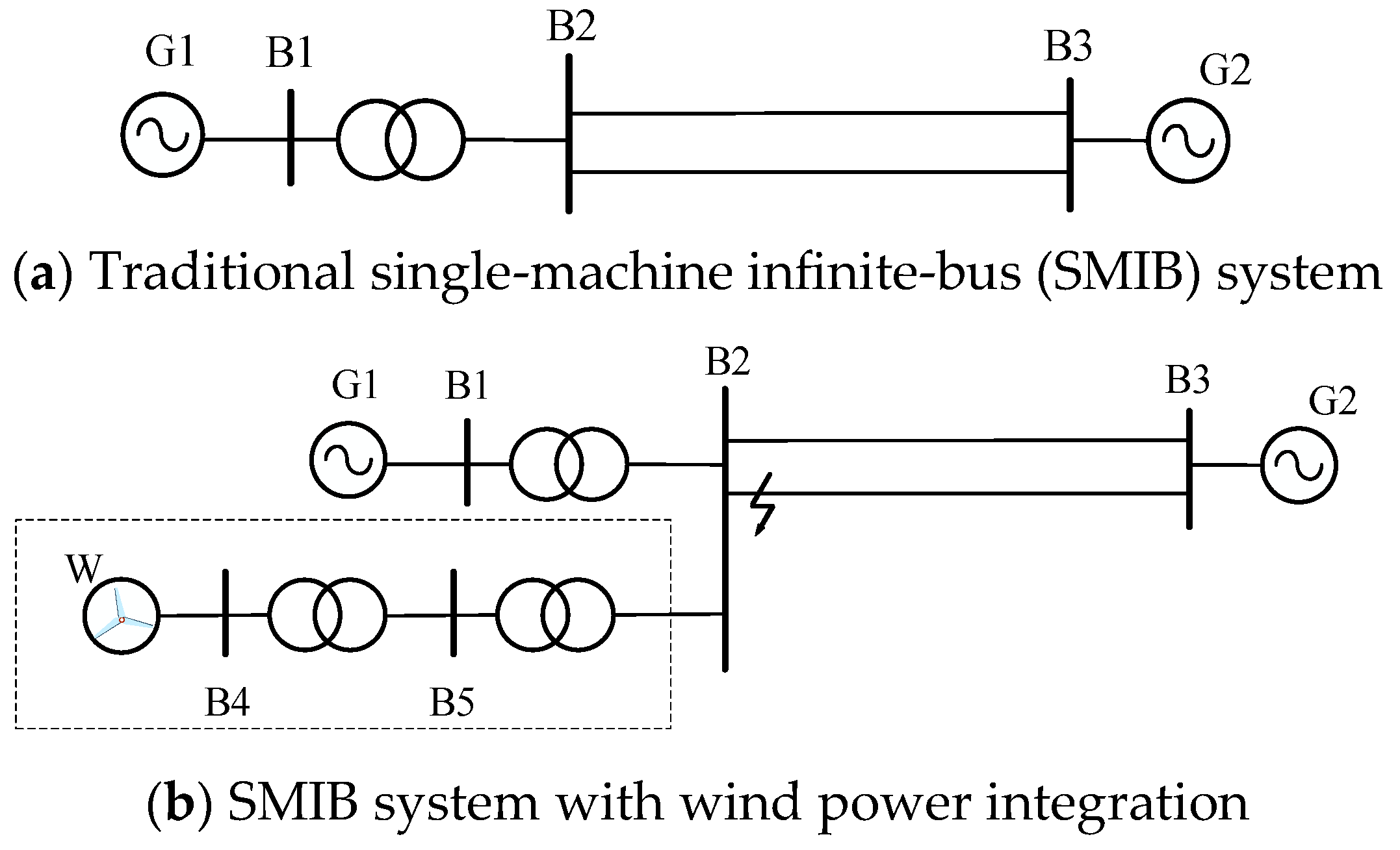
This paper investigates the impact of wind turbine active power recovery rate on system transient stability using the single-machine infinite-bus system shown in Figure 1.
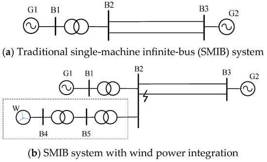
Figure 1.
Single-machine infinite-bus system.
As shown in Figure 1a, in the traditional single-machine infinite-bus (SMIB) system, a synchronous generator is connected to an “infinite bus” through equivalent impedance (including a transformer and transmission lines). The infinite bus is assumed to be an ideal voltage source with constant magnitude, fixed frequency, and zero internal impedance, unaffected by the generator’s operating state (where G1 and G2 are synchronous generators, and the infinite bus is represented by G2) [10]. A three-phase short circuit fault occurred at bus B2, with a time of 0.1 s and a duration of 0.1 s. Generator side the synchronous machine rated voltage is 20 kV, connected to a 500 kV transmission line via a step-up transformer (20 kV/500 kV). Transformer leakage reactance is 0.15 p.u. (base capacity: 100 MVA). The transmission line is a simplified equivalent model with total impedance of 0.02 + j0.50 p.u. Infinite bus voltage is 1.0 p.u. (constant). Short-circuit capacity is 10,000 MVA. The fault condition is when a three-phase short-circuit fault occurs at Bus B2. Fault initiation time is 0.1 s and the duration is 0.1 s.
In the SMIB system, the dynamic behavior of generator G1 is typically described by the rotor swing equation using the classical second-order model:
For the system shown in Figure 1, the rotor swing equation of generator G1 is as follows:
where , , M are the rotor angle, angular velocity, and inertia time constant of generator G1, respectively; Pa, PT and PE represent the accelerating power, mechanical input power, and electromagnetic output power of generator G1; and denotes the rated angular velocity of the generator.
As shown in Figure 1b, in the SMIB system with wind power integration, W represents the wind farm (80 × 5 MW doubly fed induction generators, DFIGs). During stable system operation, the electromagnetic power outputs from synchronous generators and wind turbine generators remain balanced with the power demand of the infinite bus. During stable operation, the system is consistent.
As shown in Figure 1, G1 and G2 are synchronous generators, G2 represents the infinite system, and W is the wind turbine. When the system operates stably, it always maintains the following:
where PE and Pw respectively represent the active power of synchronous machine G1 and wind turbine W, and PG2 is the active power required by the infinite system (with active losses in transformers and transmission lines neglected for simplicity).
2.1. Model of Doubly Fed Induction Generator (DFIG)
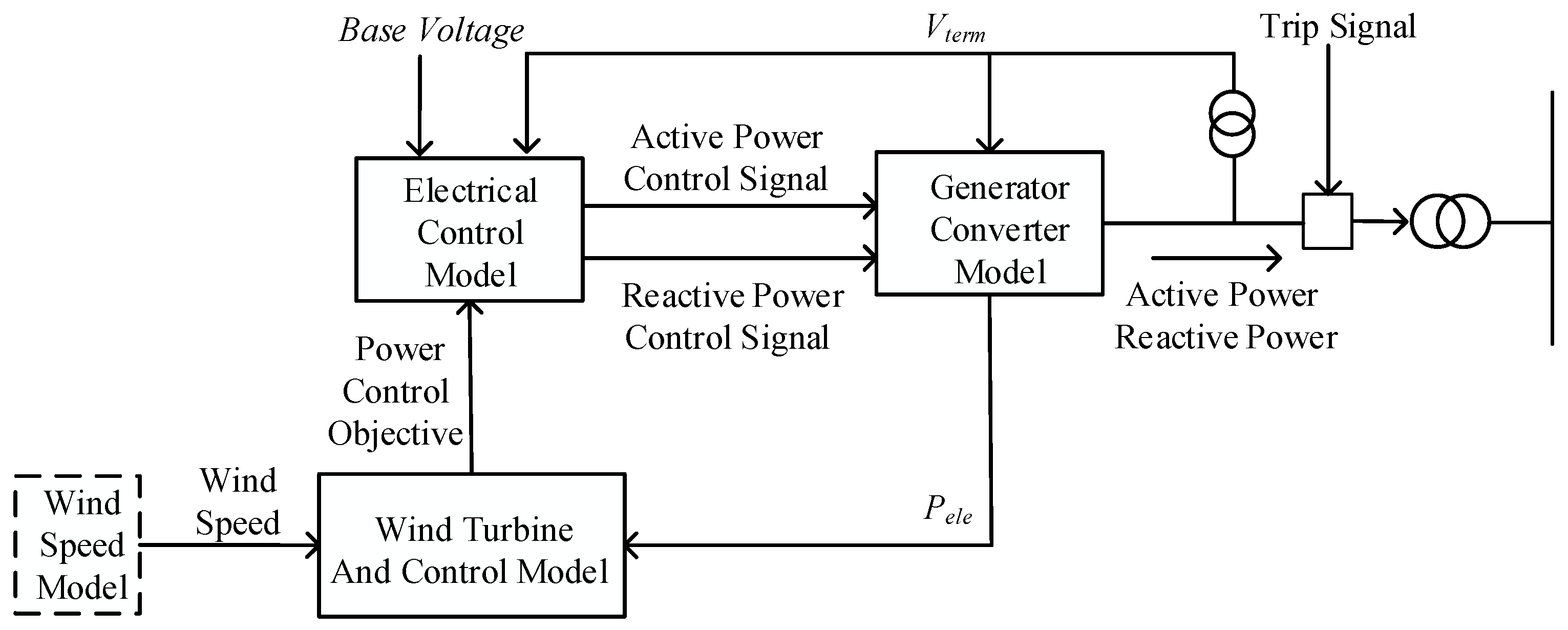
As shown in Figure 2, the wind turbine control model transmits a power control signal to the electrical control model, instructing the converter to deliver specified power to the grid according to the control signal. The electrical control model feeds the active power control signal and reactive power control signal into the generator converter model. The generator and converter behave as a current-regulated voltage source inverter, enabling the wind turbine unit to act as a controllable voltage source behind reactance, which controls the current injected by the wind turbine into the grid. Ref. [26] has demonstrated the applicability of this model in power system transient stability analysis of power systems using simulation software PSASP (7.41.04).
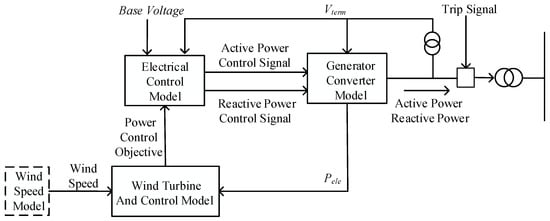
Figure 2.
Simulation model of doubly fed wind turbine.
The generator converter model includes four operational states of the wind turbine, as illustrated in Figure 3. It enables logical modeling of the complex control logic for high/low-voltage ride through (HVRT/LVRT) in the generation system, achieving stable operation of the wind turbine unit under abnormal high/low-voltage conditions.
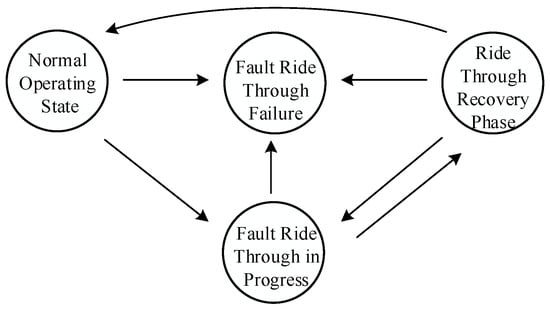
Figure 3.
The operating status of the doubly fed wind turbine.
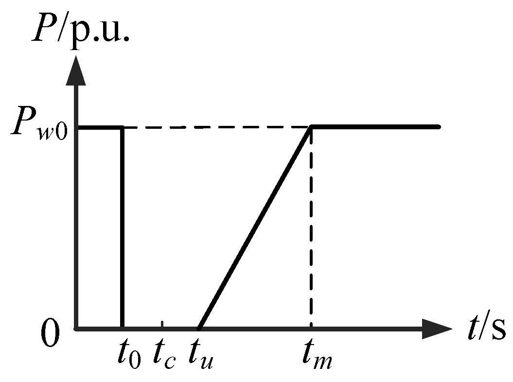
Assuming that the active power of the wind turbine before the fault is Pw0, the power drops to 0 during the fault, and the wind turbine gradually recovers to the initial power value at the preset recovery rate after the fault is cut off. The specific expression is as follows:
The active power recovery of the wind turbine is shown in Figure 4.

Figure 4.
Active power recovery process of wind turbine.
In Figure 4 and Equation (2), k is the recovery rate of active power of the wind turbine, t0 is the moment when the fault occurs, tc is the time when the fault is removed, tu is the end of the duration of the starting point of active power recovery of the wind turbine, and tm is the moment when the active power of the wind turbine recovers to the initial power value.
The active recovery control of the wind turbine directly affects the active change in the recovery process and then affects the dynamic response of the synchronous machine, resulting in the change in system transient stability.
2.2. Stability Margin Index of Trajectory Analysis Method
For the system shown in Figure 1, according to literature [25], the transient energy V of synchronous machine G1 can be expressed as:
where in Formula (4) the following can be expressed as:
where is the potential energy of synchronous machine G1 and is the kinetic energy of synchronous machine G1; and M are the rated power and inertia time constant of synchronous machine G1, respectively; and and are the acceleration power and angular velocity of synchronous machine G1, respectively.
The moment when synchronous machine G1 first reaches its minimum potential energy is , and the moment when it first reaches its maximum potential energy is . At time , the stability margin index [26] of synchronous machine G1 is as follows:
where is the potential energy increment of generator G1.
2.3. Construction of Sensitivity Model
Combined with the stability margin index, the sensitivity model of the stability margin index to the active power recovery rate of wind turbine can be established so as to analyze the influence of the active power recovery rate on the stability margin index.
For the system shown in Figure 1, the sensitivity mathematical model of the transient stability margin index to the active power recovery rate of wind power is defined by combining Equations (5) and (6) as follows:
Combining Formulas (1), (3), and (5), the following can be concluded:
where Pa(t) = kPw0(t − tu) − PG2 + PT. Among them, reflects the impact of changes in the active recovery rate of the wind turbine on the power balance of the synchronous machine; and reflects the influence of changes in the active recovery rate of the wind turbine on the transient potential energy change rate of the system, including how the recovery rate affects the potential energy change rate through changes in the synchronous machine’s acceleration power and speed.
By substituting Formula (8) into Formula (7) and organizing it, the following can be concluded (detailed derivation process can be found in Formulas (A6)–(A15) in Appendix A.1):
In Formula (9), the following are expressed as:
where N1, N2, and N3 are related to the change in potential energy , and N4, N5, and N6 are related to the time .
Among them, f1(k) represents the impact of the change in the active recovery rate of the wind turbine on the acceleration power of generator G1, which directly causes the change in system sensitivity; f2(k) and f3(k), respectively, represent the direct impact of the change in the active recovery rate of the wind turbine on the acceleration power and speed of generator G1, leading to changes in potential energy and indirectly causing changes in sensitivity.
In multi-machine systems with wind power integration, the active power balance relationship between wind turbines and synchronous generators is expressed as:
where PEi is the active power output of synchronous generator i; Ploss is the total active power loss in the system; and Pload is the total active load power in the system.
It is assumed that the electromagnetic power output of generator i is influenced by wind power integration and becomes the following:
where αi represents the proportional relationship between the active power output of generator i and the total active power output of all synchronous generators after wind turbine integration, with 0 ≤ αi ≤ 1.
Building on the sensitivity model developed for single-machine systems, the sensitivity mathematical model of the transient stability margin index to the wind power active recovery rate in multi-machine systems is derived as follows (detailed derivation in Appendix A.2):
The sensitivity of the stability index to the active power recovery rate of wind turbines reflects the impact of changes in the active power recovery rate on system stability. It quantifies how changes in the active power recovery rate k affect the stability margin index S. If ∂S/∂k < 0, it indicates that as the active power recovery rate k increases, the stability index S decreases, meaning system stability improves and suggesting that an increase in k has a negative impact on system stability. If ∂S/∂k > 0, it indicates that as k increases, the stability index S increases, meaning system stability improves and suggesting that an increase in k has a positive impact on system stability. If ∂S/∂k = 0, it means that changes in k have no effect on the stability index S, indicating that system stability is unaffected by changes in k.
3. Results
Considering the factors affecting the stability of the system, this section will analyze the active power recovery rate of wind turbines, the initial active power output, and the fault duration from three aspects.
3.1. Analysis of the Influence of the Active Recovery Rate of Wind Turbine on System Stability
- (1)
- Accelerating power of synchronous machine
According to Formula (A1) in Appendix A.1: . Therefore, after the fault is cleared, when the active power recovery rate k of the wind turbine increases, the acceleration power of the synchronous machine will increase. This is because the rapid recovery of active power from the wind turbine reduces the power difference that the synchronous machine needs to bear, thereby decreasing PE and increasing the acceleration power.
- (2)
- The speed of the synchronous machine
According to Formula (A4) in Appendix A.1, it can be seen that . This indicates that after fault removal, when the active recovery slope k of the wind turbine increases, the acceleration power of the synchronous machine increases but gradually decreases, thus leading to a slower change in its speed.
- (3)
- The change in potential energy and power angle of the synchronous machine
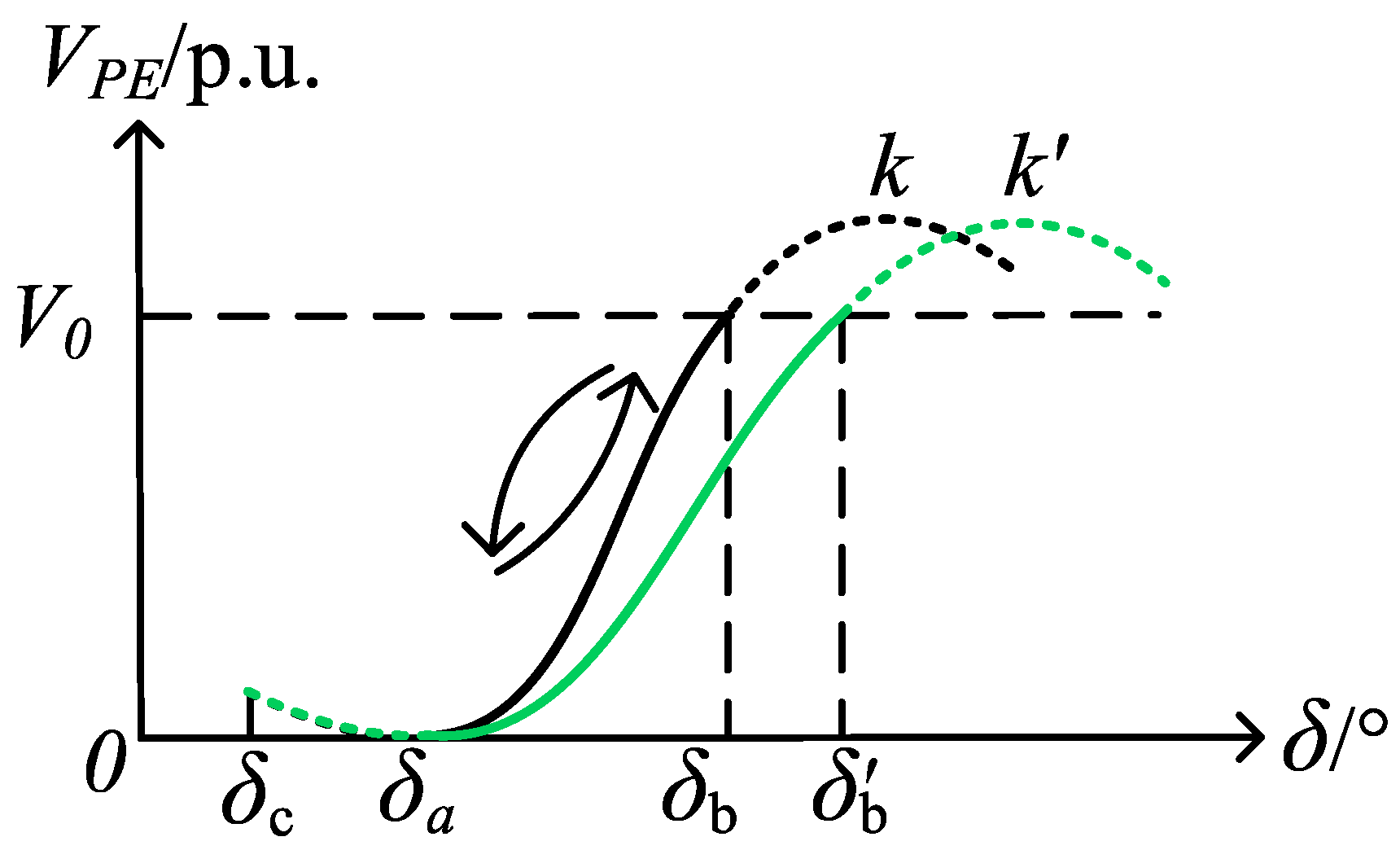
The change in potential energy is the amount of potential energy that changes after the synchronous machine has been tripped from a fault. It reflects the energy conversion situation during the transient process of the system. In Figure 5, the black line and green line represent the transient potential energy changes in the synchronous machine G1 under two conditions: when the active power recovery slope of the wind turbine is k and k′, respectively, with k < k′. Furthermore, points and in Figure 5 represent the rotor angles of synchronous generator G1 at times tc and ta, respectively, while points and denote the rotor angles of synchronous generator G1 at time tb under active power recovery rates k and k′ of the wind turbine, respectively.

Figure 5.
Potential energy change in the synchronous machine in steady state.
According to Formula (4), during the fault process the active power recovery rate of the wind turbine does not affect the dynamic behavior of the synchronous motor. Therefore, the total transient kinetic energy accumulated by the synchronous motor during the fault phase remains unchanged and the peak potential energy also remains constant. The magnitude of the change in potential energy is not directly influenced by the active power recovery rate of the wind turbine. However, . This indicates that as the active power recovery slope k of the wind turbine increases, the rate of change in potential energy of the synchronous motor gradually decreases. Since the magnitude of the first peak in potential energy does not change, the power angle corresponding to the peak potential energy will increase accordingly.
- (4)
- The time when the potential energy of the synchronous machine reaches its peak for the first time
The power variation characteristics of the wind turbine determine that the active power will not immediately recover to the initial power after fault removal, but will go through a process from the fault crossing stage to the fault recovery state and finally recover to the initial active power at the time point tm.
When the time tb is within the interval , the active power of the wind turbine remains at zero. Therefore, changes in the active recovery slope k do not affect system stability. When time , changes in the active recovery rate k will impact the time at which potential energy reaches its peak. At time tb, if the synchronous generator can maintain stability, it must satisfy . Since the speed of the synchronous generator decreases more slowly as k increases, the time tb after fault clearance for the synchronous generator’s speed to drop to zero will also be extended accordingly. This indicates that with an increase in the active recovery slope of the wind turbine, the rate of change in the synchronous generator’s potential energy decreases, leading to a delay in the time at which the potential energy reaches its peak.
- (5)
- Stability index of synchronous machine
According to Formula (6), . Under unchanged fault conditions, the change in potential energy of the synchronous machine, , remains constant; however, an increase in the active power recovery slope k of the wind turbine leads to an increase in the acceleration power at time , with its absolute value gradually decreasing. Therefore, the stability index S decreases as the active power recovery slope k of the wind turbine increases.
In summary, an increase in the active recovery rate k of the wind turbine will reduce the potential energy change rate of the synchronous generator, leading to a larger power angle at the peak of potential energy and a longer duration. The synchronous generator will also recover to its pre-fault power balance state more quickly, but its stability margin gradually decreases. This phenomenon indicates that while a higher active recovery rate of the wind turbine can help to rapidly restore power balance, an excessively fast recovery rate may adversely affect the transient stability of the synchronous generator.
3.2. Analysis of the Influence of the Initial Active Power of the Wind Turbine on the Stability of the System
- (1)
- The acceleration power of the synchronous machine
According to Formula (A2) in Appendix A.1: . When t < tb then there is k(ΔPw0)(t − tu) < ΔPG2. Consequently, with the increase in the initial active power Pw0 of the wind turbine, the acceleration power Pa(t) of the synchronous machine will increase. Under the same active recovery rate, the initial active power of the wind turbine increases, resulting in an increase in the power difference (PG2 − Pw) that the synchronous turbine needs to bear and thereby increasing the PE and reducing the acceleration power.
- (2)
- The change in potential energy
According to the above analysis, the magnitude of the potential energy change of the synchronous machine is not directly affected by the initial active power of wind power. According to Equation (4), . Since the initial active power of the wind turbine decreases under the same active recovery rate, the acceleration power of the synchronous machine increases, the potential energy change rate gradually accelerates, and the corresponding power angle when the potential energy reaches the peak will decrease.
- (3)
- The time when the potential energy of the synchronous machine reaches its peak for the first time tb
According to the above analysis, if the synchronous machine can remain stable at the tb time then must be satisfied. Due to the fact that the initial active power of the wind turbine decreases under the same active recovery rate of the wind turbine, the acceleration power of the synchronous turbine increases but gradually decreases. Consequently, when the fault is removed the time for the speed of the synchronous machine to drop to zero is correspondingly shortened. This shows that with the increase in the initial active power of the wind turbine the potential energy change rate of the synchronous turbine accelerates and the potential energy peak time is shortened.
- (4)
- The stability index S of the synchronous machine
According to Equation (6), . Under the condition that the fault condition is unchanged, the potential energy change of the synchronous machine remains unchanged. However, the increase in the initial active power Pw0 of the wind turbine will reduce the acceleration power of the synchronous generator at the tb time, and its absolute value is gradually increasing. As such, the stability index increases with the increase in the initial active power of the wind turbine.
3.3. Analysis of the Impact of Fault Duration on System Stability
- (1)
- The acceleration power of the synchronous machine
According to Formula (A2) in Appendix A.1, it can be seen that . If the fault duration increases, the active recovery time of the wind turbine will be delayed and the acceleration power of the synchronous machine will decrease. The longer the fault duration of the wind turbine under the same active recovery rate, the power difference (PG2 − Pw) that the synchronous machine needs to bear increases, thereby increasing the PE and reducing the acceleration power.
- (2)
- The change in potential energy
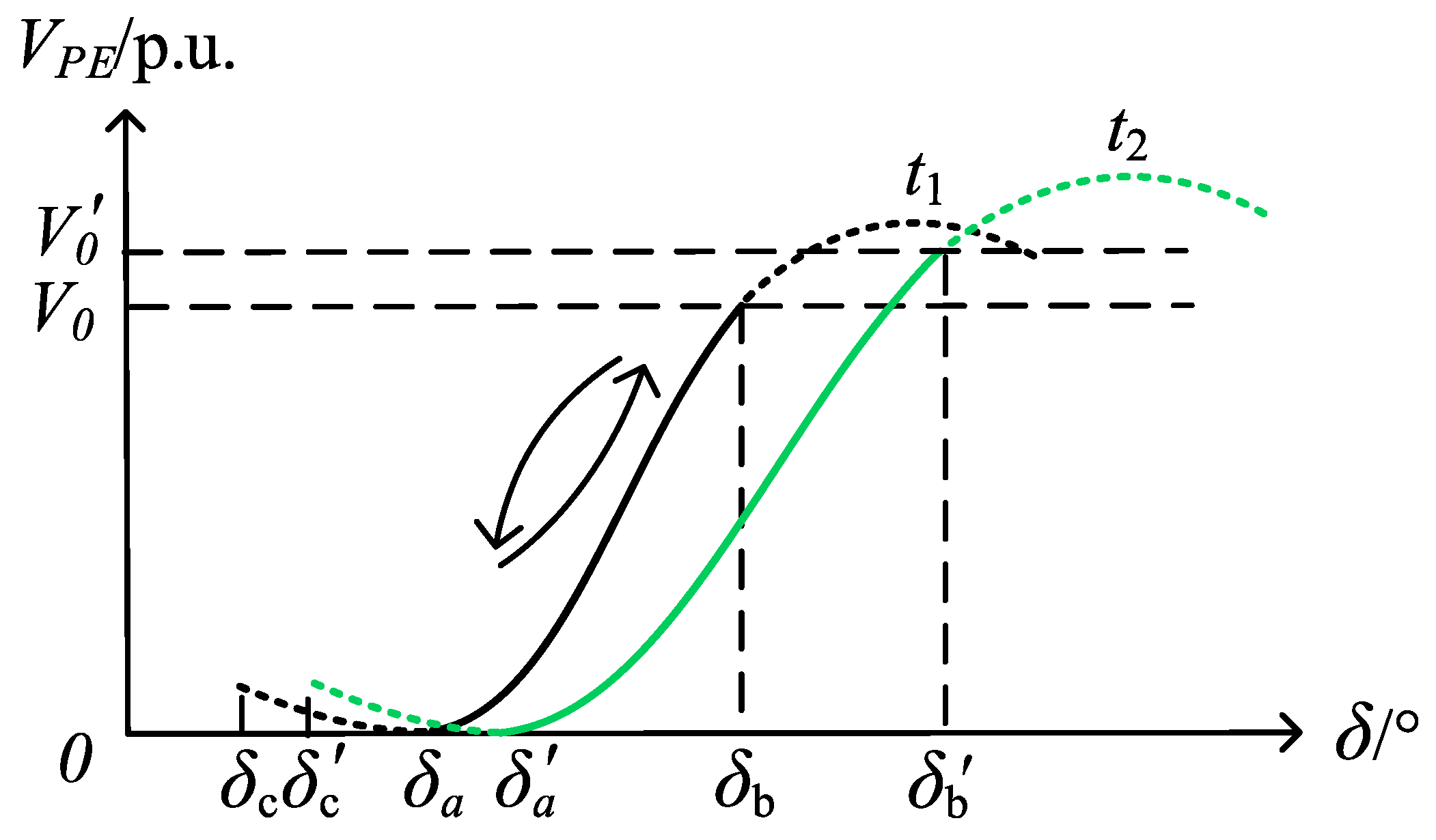
In Figure 6, the black and green lines represent the transient potential performance changes in the synchronizer when the fault duration is t1 and t2, respectively, and t1 < t2. Additionally, points , , and in Figure 6 correspond to the rotor angles of synchronous generator G1 at times tc, ta, and tb, respectively, when the fault clearance time is t1. Similarly, points , , and represent the rotor angles of synchronous generator G1 at times tc, ta, and tb, respectively, under a fault clearance time of t2.
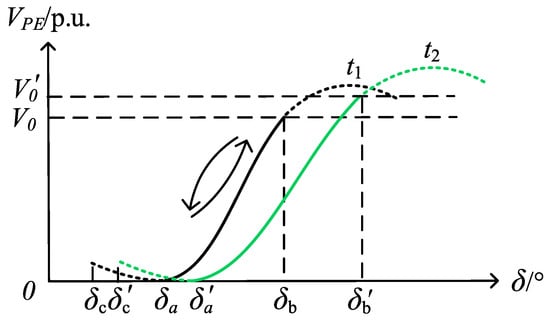
Figure 6.
The change in potential energy of the synchronizer under different fault durations.
The increase in fault duration leads to an increase in the power angle of the synchronizer at the time of fault removal, and the time when the potential energy reaches the minimum value for the first time after the fault resection is delayed. Since , an increase in the fault duration leads to a decrease in the acceleration power of the synchronous machine, and the rate of change in its potential energy gradually decreases. In addition, an increase in fault duration leads to an increase in the accumulation of synchronous maneuver energy during the fault period. Therefore, when the potential energy reaches the peak, the corresponding power angle will increase with an increase in fault duration. The potential energy variation curve of the synchronous machine is shown in Figure 4.
- (3)
- The time when the potential energy of the synchronous machine reaches its peak for the first time tb
According to the above analysis, at the tb moment, an increase in the duration of the failure leads to a decrease in the acceleration power of the synchronizer, but as , which gradually maximizes, the time when the speed of the synchronous machine drops to zero after the fault is removed will also be delayed accordingly. In addition, the prolongation of the fault duration indicates that the recovery process of potential energy after fault removal is delayed, and the time tb is further increased.
- (4)
- The stability index S of the synchronous machine
According to Equation (6), . According to the above analysis, an increase in fault duration leads to a decrease in the acceleration power of the synchronous machine, a decrease in the accelerating power of the synchronous machine at the tb moment, and an increase in potential energy change. Therefore, the stability index decreases with an increase in the fault duration, and the stability of the system gradually decreases.
In summary, an increase in fault duration reduces the rate of potential energy variation in synchronous generators, leading to an enlarged rotor angle and delayed timing when the potential energy reaches its peak. This results in a gradual decrease in the stability margin index and degradation of system stability.
This section investigates the impacts of three factors—active power recovery rate, initial active power of wind turbines, and fault duration—on system transient stability.
Increasing the active power recovery rate accelerates power balance restoration but slows the rate of potential energy variation in synchronous generators. This delays the occurrence of the potential energy peak, amplifies rotor angle deviations, and reduces the stability margin index. These effects indicate that excessively fast recovery rates may exacerbate source–grid dynamic mismatch.
Enhancing the initial active power improves dynamic energy regulation, shortening the time to reach the potential energy peak and reducing rotor angle deviations, thereby increasing the stability margin index. However, high initial power output requires caution due to risks of insufficient inertia support.
Prolonging fault duration accumulates more transient kinetic energy, expands the magnitude of potential energy variation, delays peak timing, and significantly weakens the system stability margin.
4. Discussion
4.1. Single-Machine System Simulation Analysis
In the stand-alone infinity system with wind turbine access shown in Figure 1, a three-symmetrical short-circuit fault occurs at the Bus2 node when the fault start time is set to 0.1 s, the simulation time is 5 s, and the step size is 0.01 s. To validate the above analysis, we set up the following scenarios:
Scenario 1: If the fault duration is 0.1 s and the active power output of the wind turbine is 200 MW, the active power recovery rate of the wind turbine is changed to 0.1 p.u./s, 0.2 p.u./s, and 0.3 p.u./s.
Scenario 2: The fault duration is 0.1 s, the active recovery rate of the wind turbine is 0.2 p.u./s, and the active output of the wind turbine is changed to 100 MW, 200 MW, and 300 MW.
Scenario 3: The active power output of the wind turbine is 200 MW, the active power recovery rate of the wind turbine is 0.2 p.u./s, and the fault duration is changed to 0.1 s, 0.12 s, and 0.15 s.
Table 1 variables translation: “Sensitivity ∂S/∂k” refers to the sensitivity model proposed in the paper; “Stable index S” refers to the stability indicator proposed in Section 2.2 of the paper for determining system stability margin; “Power angle (°)” indicates the power angle of the generator; “Accelerating power (p.u)” represents the difference between mechanical power and active power of synchronous machines; and “Time tb(s)” denotes the time when potential energy first reaches its maximum value. The variable meanings in subsequent tables maintain the same definitions as those in Table 1.

Table 1.
Simulation results of the physical quantities of the synchronous machine in scenario 1.
According to Table 1, with an increase in the k value, the rapid recovery of the active power of the wind turbine reduces the power difference that the synchronous machine needs to bear, which leads to a decrease in the acceleration power amplitude of the synchronous turbine and alleviates the electromagnetic power imbalance of the synchronous machine. This also causes the speed and potential energy change rate of the synchronous machine to decrease, resulting in the power angle shifting backward when the potential energy of the synchronous machine reaches the peak, and at the same time delaying the arrival time of the peak potential energy tb.
As indicated in Table 2, an increase in the initial power output of wind turbine generators progressively elevates the sensitivity of synchronous machines, while simultaneously reducing the magnitude of the transient stability index. This is accompanied by an expanded rotor angle , diminished accelerating power , and shortened time to reach peak potential energy in the transient energy function. These coordinated dynamics conclusively demonstrate that higher initial wind power injection degrades system transient stability.
Table 2.
Simulation results of the physical quantities of the synchronous machine in scenario 2.
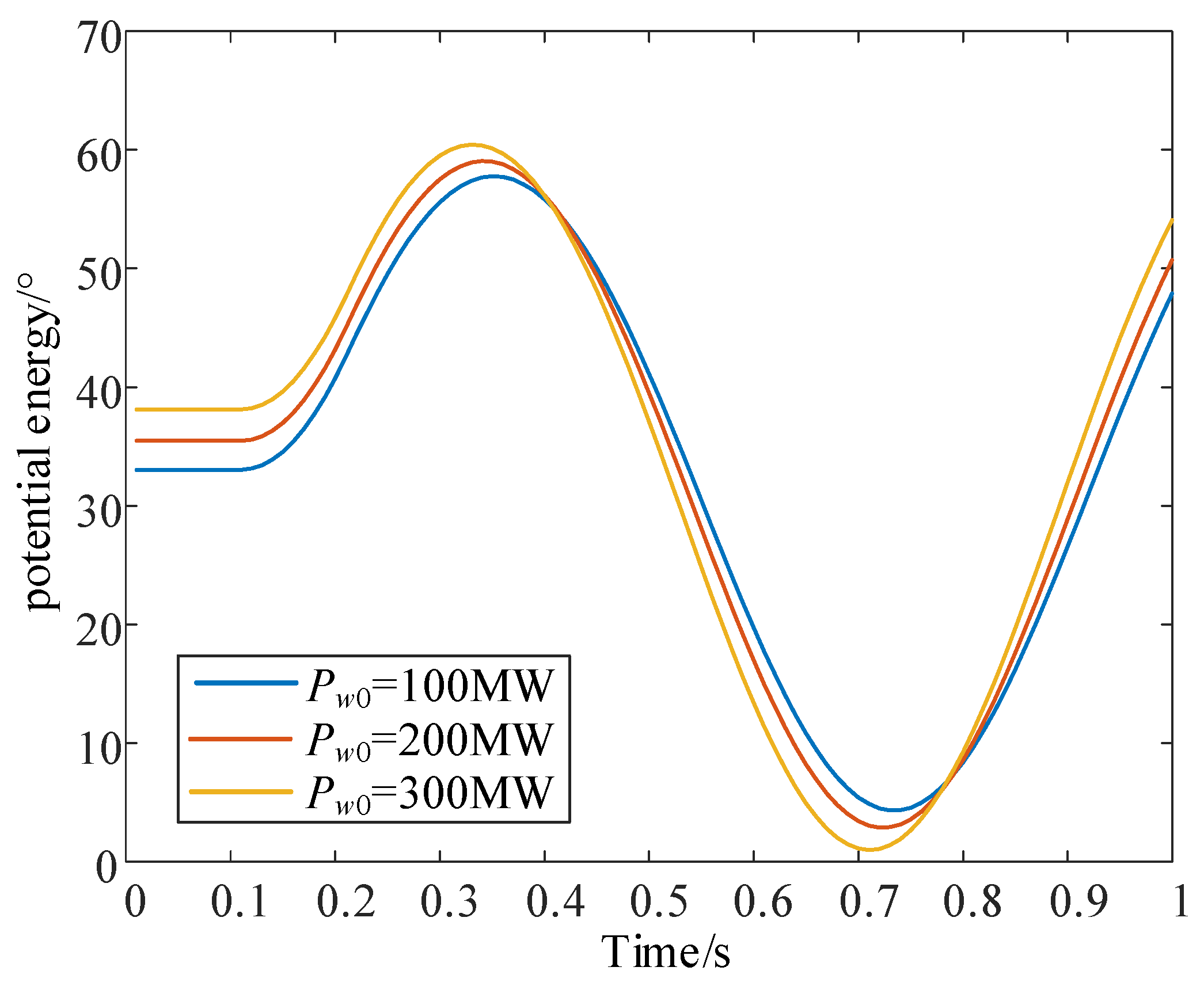
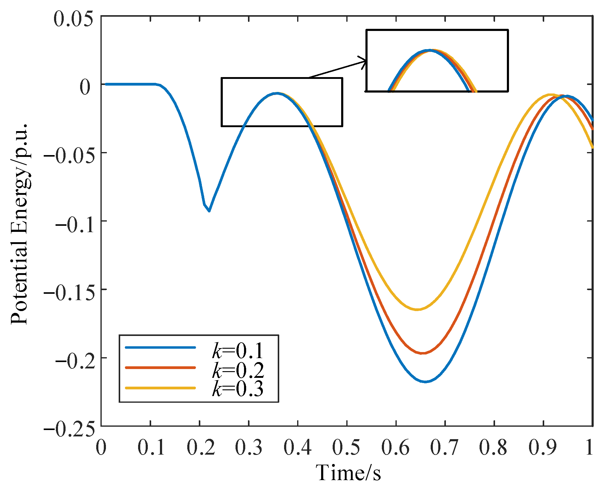
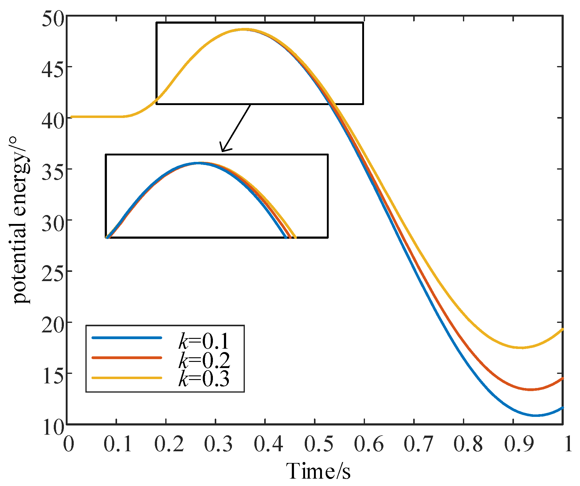
Considering that the fault duration is 0.1 s and the active recovery rate of the wind turbine is 0.5 p.u./s, the potential energy and power angle variation curves of the synchronous machine under the initial active power of different wind turbines are shown in Figure 7 and Figure 8. In Figure 7, the potential energy reaches a minimum for the first time about 0.2 s after the fault is removed and peaks at around 0.36 s. With the increase in the initial active power of the wind turbine, the time when the potential energy reaches the peak time Tb will gradually shorten but the peak amplitude will remain constant, indicating that the potential energy change rate accelerates with the increase in the initial power of the wind turbine. In Figure 8, an increase in the initial power of the wind turbine first leads to an increase in the initial power angle of the synchronizer. In addition, the time required for the power angle to reach the peak decreases with the increase in the initial power, but the difference between the peak and the initial angle shows a decreasing trend and the attenuation of the power angle oscillation amplitude indicates that the transient stability of the system is enhanced.
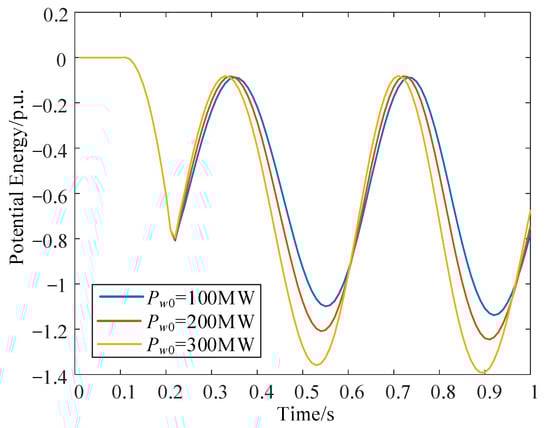
Figure 7.
Potential energy curves of synchronous machines under the initial active power of different wind turbines.
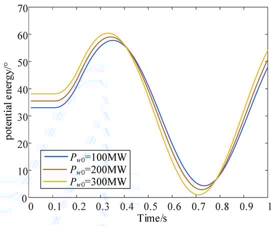
Figure 8.
The power angle variation curve of the synchronous machine under the initial active power of different wind turbines.
As demonstrated in Table 3, prolonged fault duration leads to a progressive decline in sensitivity and stability index magnitude, accompanied by an increase in rotor angle , a reduction in accelerating power , and delayed time to peak potential energy in the transient energy function. These coordinated trends conclusively indicate a systematic deterioration of system transient stability.
Table 3.
Simulation results of the physical quantities of the synchronous machine in scenario 3.
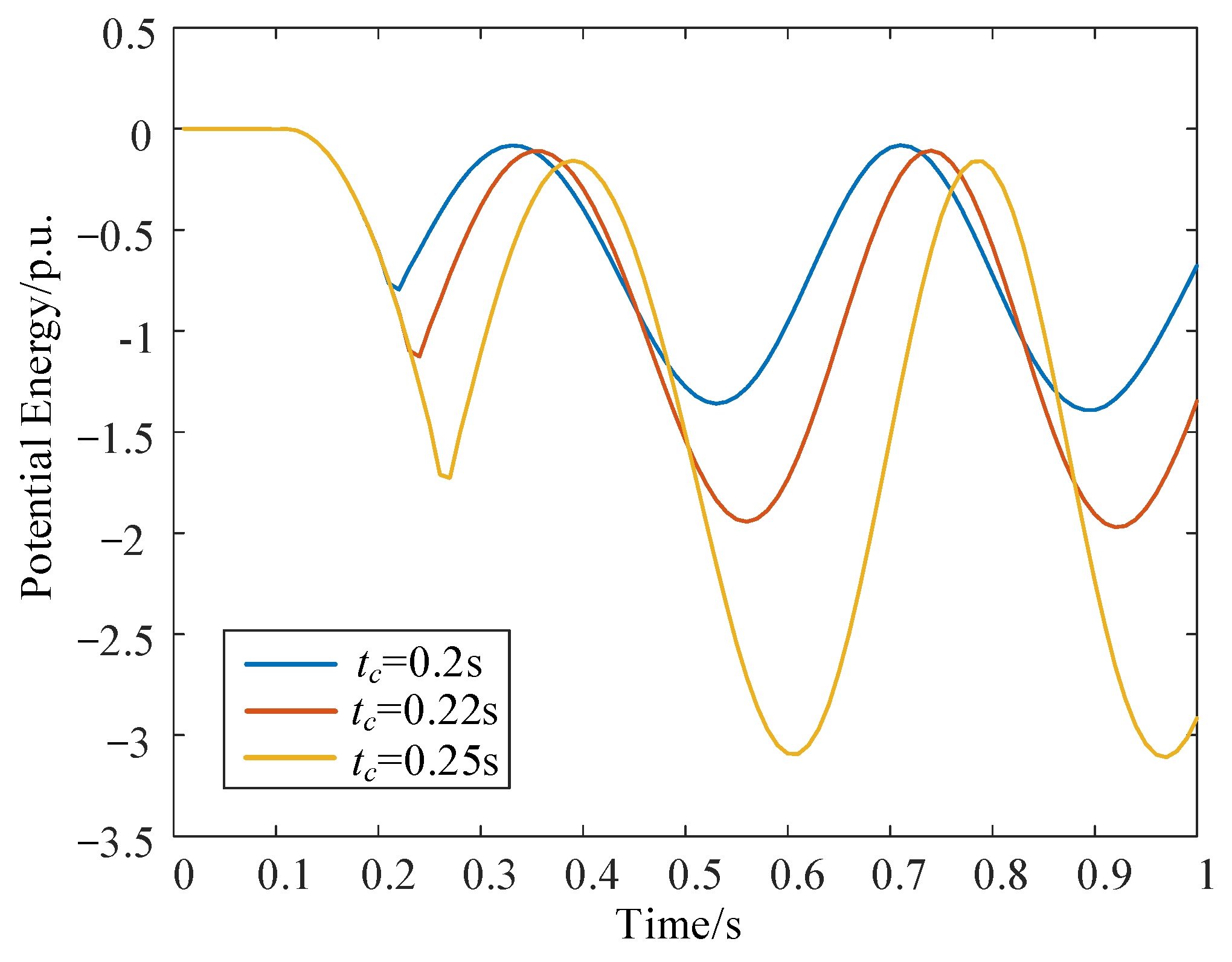
Considering that the initial active power of the wind turbine is 400 MW and the active recovery rate is 0.2 p.u./s, the potential energy and power angle variation curves of the synchronous machine under different fault durations are shown in Figure 9 and Figure 10. In Figure 9, with an extension of the fault duration, the fluctuation amplitude of the potential energy of the synchronous machine from the minimum value to the maximum value for the first time gradually increases and the time for the potential energy to reach the peak is delayed accordingly, indicating that an increase in the fault duration leads to a significant increase in the kinetic energy accumulated by the synchronous machine during the fault period. In Figure 10, an increase in the fault duration leads to an increase in the amplitude of the power angle, resulting in a decrease in system stability.
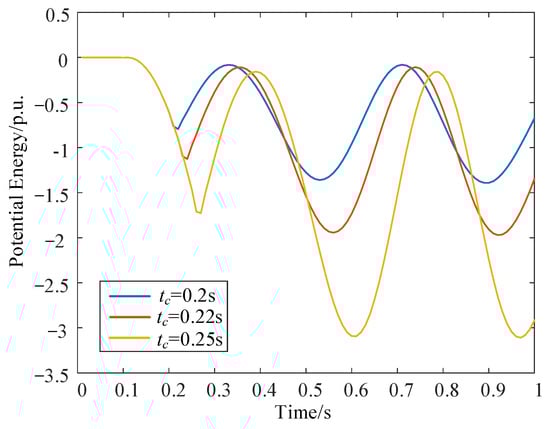
Figure 9.
The potential energy variation curve of synchronous motor under different fault durations.
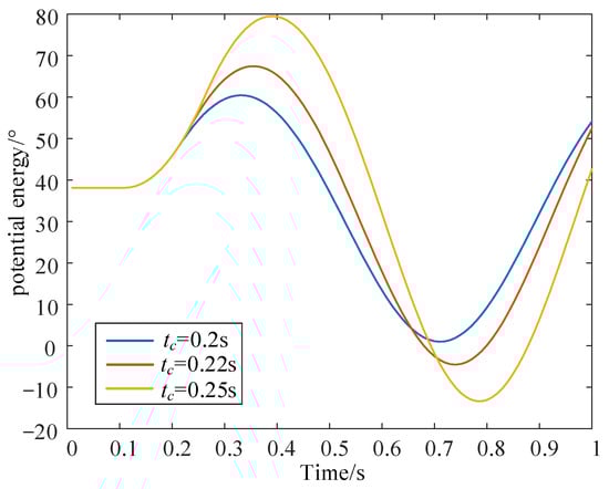
Figure 10.
The power angle variation curve of synchronous motor under different fault durations.
4.2. Multi-Machine System Simulation Analysis
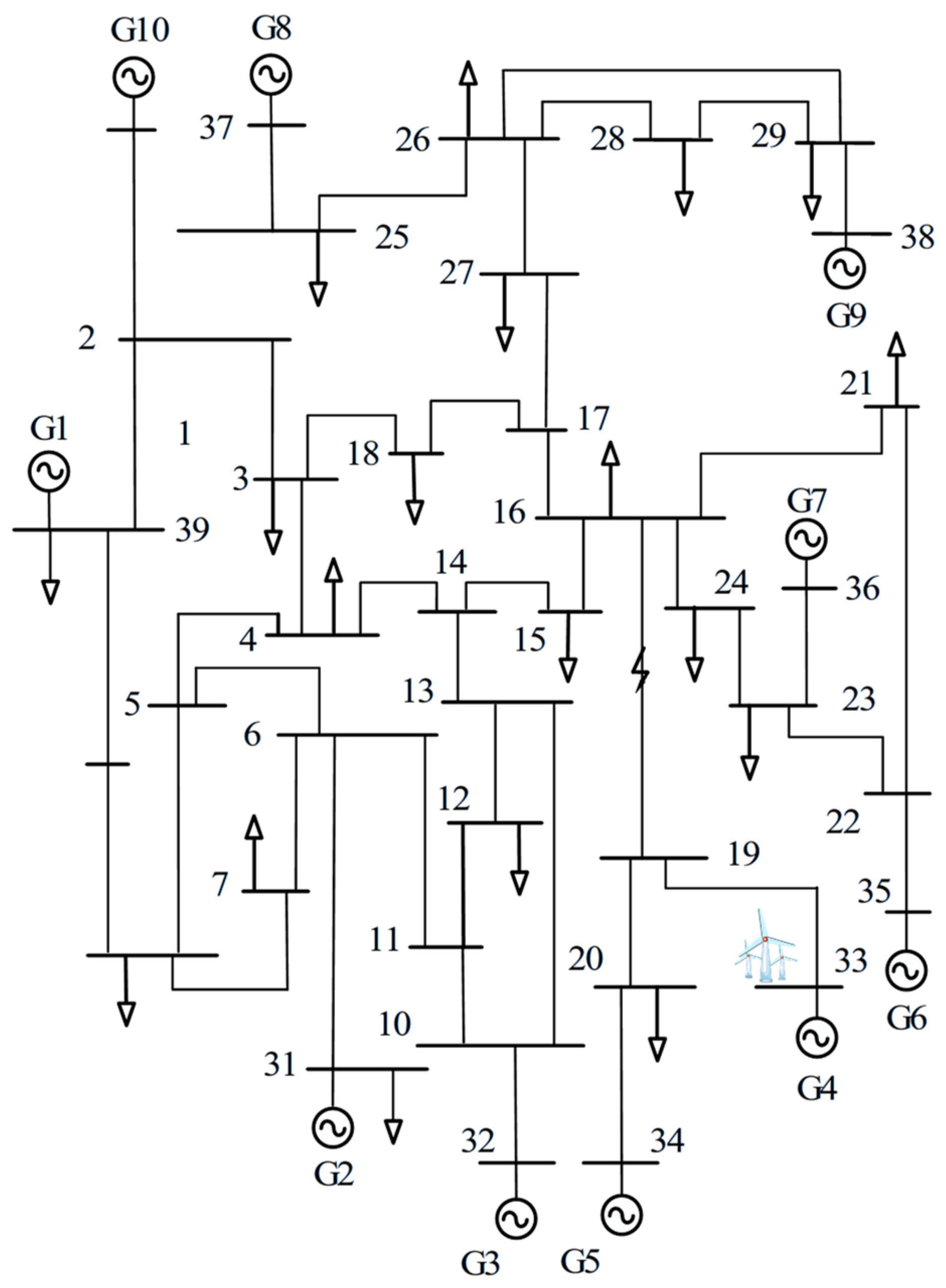
This section conducts simulation verification based on the 10-machine 39-bus standard test system, with its topology shown in Figure 11. The network comprises 10 classical second-order synchronous generators (G1–G10) and 19 constant-impedance load buses.
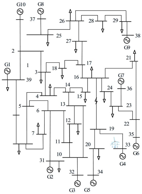
Figure 11.
10-generator 39-bus test case system.
The study selects Bus33 as the wind power integration point, configured with an initial wind power output of 300 MW. A three-phase symmetrical short-circuit fault is simulated between Bus17 and Bus19, lasting 5 s. The fault initiation time is set to 0.1 s, and the fault clearance time is 0.2 s. By varying the active power recovery ramp rate of the wind turbine (0.1 p.u./s, 0.2 p.u./s, and 0.3 p.u./s), the following simulation results are obtained. After fault clearance, the wind turbine begins gradual active power recovery at approximately 0.29 s, while the potential energy of the critical generator reaches its peak around 0.38 s. Variations in the wind turbine’s active power recovery ramp rate affect the critical generator’s dynamics
In Table 4, relevant patterns were obtained by analyzing the transient processes at different active recovery rates. The rotor angle exhibits a monotonically increasing trend, indicating that faster power recovery slightly enlarges rotor angle swings. The absolute value of accelerating power continuously decreases, demonstrating that a higher k effectively reduces transient accelerating energy. As k increases, the absolute sensitivity |∂S/∂k| decreases (∂S/∂k < 0), suggesting a diminishing impact of k on system stability. However, both the stability margin index and critical clearing time decline with increasing k, confirming that a higher k adversely affects stability in multi-machine systems.
Table 4.
Simulation results of critical generator G4’s physical quantities under different active power recovery rates.
As shown in the data in Table 5, with an increase in the active power recovery rate (k) of the wind turbine, the absolute sensitivity of all three generators exhibits a significant downward trend. Notably, generator G8 consistently demonstrates the highest sensitivity, indicating its strongest responsiveness to wind turbine power regulation. Changes in the wind turbine’s active power recovery rate exert a greater impact on synchronous generator G8 compared to others. Regarding stability indices, the stability indices of G4 and G5 decrease as k increases, indicating that raising the active power recovery rate reduces the stability of these two units. Although the stability index of G8 declines markedly, it remains at a relatively high level, suggesting better stability robustness compared to G4 and G5. However, overall, increasing k degrades system stability.
Table 5.
Stability indices and sensitivities of G4, G5, and G8 under different active power recovery rates.
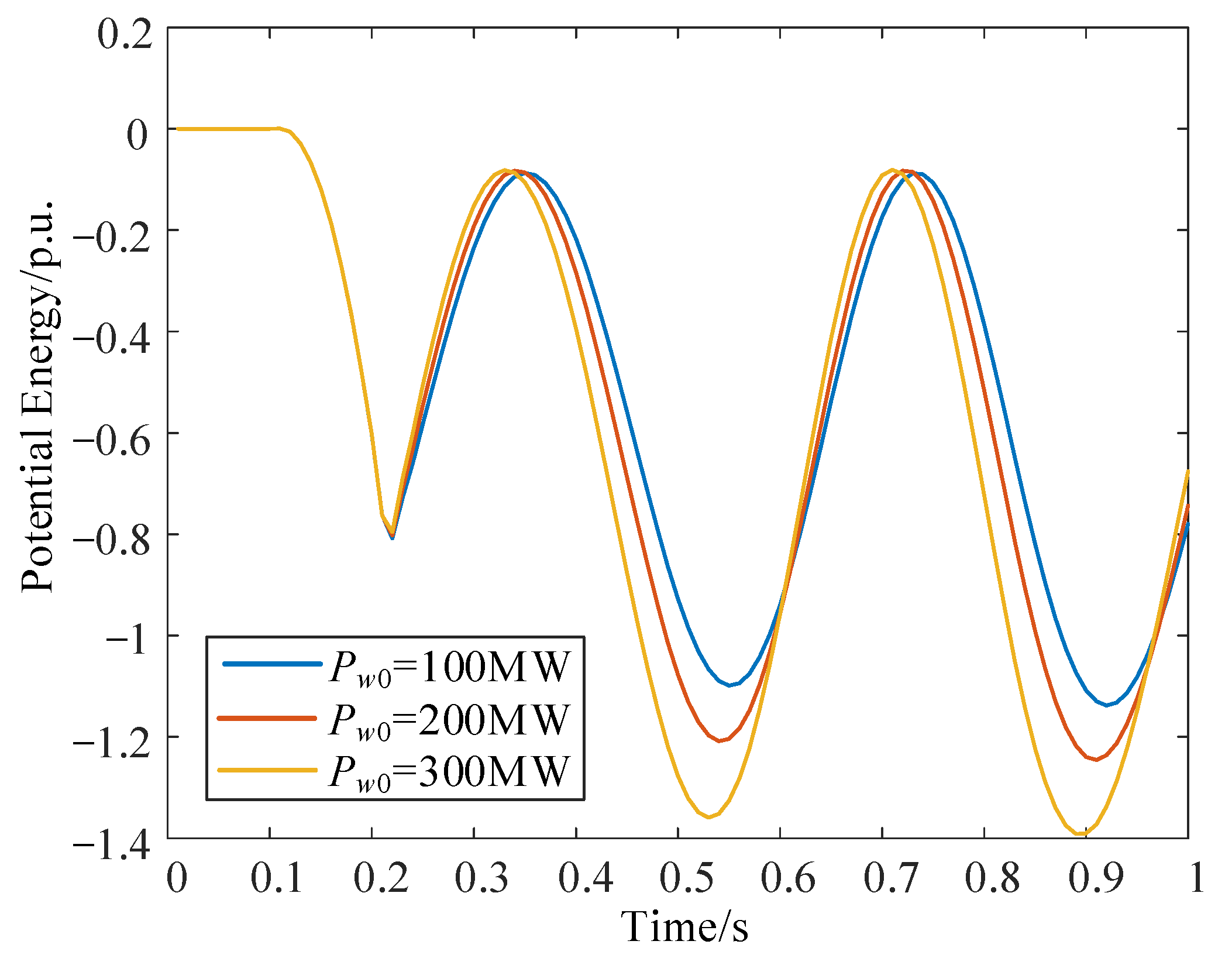
As shown in Figure 12, after fault clearance the potential energy first reaches its minimum value at 0.2 s. The potential energy attains its first maximum value around 0.38 s. Beyond 0.26 s, as the active power of the wind turbine gradually recovers, the rate of potential energy variation progressively decreases with an increase in the active power recovery ramp rate of the wind turbine. This results in variations in the peak timing tb. However, when the active power recovery ramp rate is small, its impact on rotor speed is negligible and no significant shift in tb occurs.
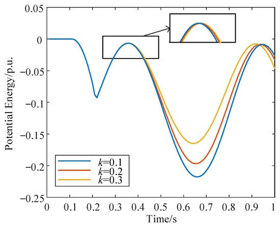
Figure 12.
Potential energy variation curve of critical machine G4.
As shown in Figure 13, after the fault occurs, the rotor angle of the critical generator gradually increases. Post-fault clearance, the rotor angle continues to rise due to the rotor speed remaining above synchronous speed, reaching its peak around 0.38 s—which is synchronized with the potential energy peak timing.
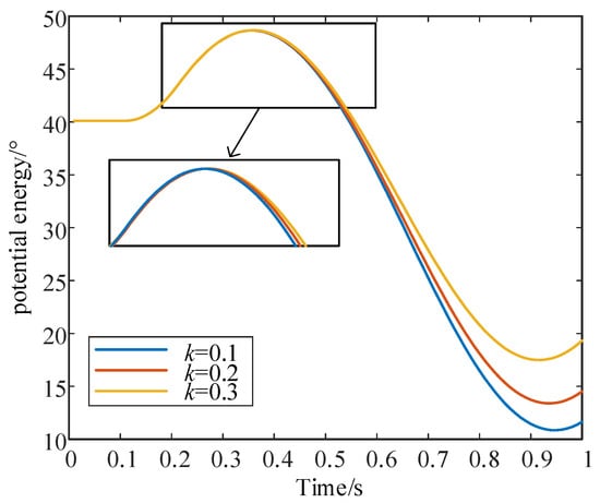
Figure 13.
Power angle variation curve of critical machine G4.
Beyond 0.26 s, as the wind turbine’s active power recovers, the rotor angle peak increases progressively with higher active power recovery rates. The increase in accelerating power of the critical generator accelerates the rate of rotor speed variation, further amplifying the rotor angle. Concurrently, the timing tb of the first potential energy peak exhibits a delaying trend.
In summary, this study reveals a non-monotonic relationship between the active power recovery rate of doubly fed induction generators (DFIGs) and system transient stability. Contrary to conventional understanding, while accelerating the active power recovery rate shortens the duration of synchronous generator accelerating power, trajectory sensitivity analysis uncovers its mechanism of reducing the rate of transient potential energy variation and delaying potential energy peaks. However, this research focuses solely on the impact of wind turbine active power recovery rates using a time-varying active power model, neglecting critical variables such as reactive power and voltage dynamics during fault recovery. Consequently, the model fails to fully capture the dynamic behavior of wind turbines during fault recovery, presenting limitations. Future studies should address these aspects.
5. Conclusions
By constructing a sensitivity model of the stability margin index to the active power recovery rate of wind turbines, this paper elucidates the mechanism by which wind power active recovery dynamics influence power system transient stability. Key conclusions are as follows:
A 0.1 p.u./s increase in the active power recovery rate results in a stability margin index reduction of approximately 0.014 in the single-machine system, accompanied by a decrease in absolute sensitivity magnitude of about 0.997, indicating a nonlinear negative correlation between the recovery rate and stability margin. In multi-machine systems, the critical generator G8 exhibits the highest sensitivity, with its stability index declining by 23.5% as parameter k increases. Enhancing the recovery rate elevates the synchronous machine accelerating power by 12.7%, amplifies rotor angle peak deviation by 2.4%, and delays potential energy peak time by 0.02 s, thereby validating the “accelerating power-potential energy time delay” coupling mechanism.
Increasing the active power recovery rate of wind turbines leads to an increase in synchronous generator accelerating power; a slowed rotor speed deceleration rate; a rise in rotor angle peaks; a decline in the rate of potential energy variation (while the total potential energy variation remains constant); and a reduction in the system stability margin index, thereby degrading system stability.
The impact of the active recovery rate on the stability margin exhibits a nonlinear trend, initially increasing and then decreasing as the recovery rate rises. Higher initial active power output from wind turbines suppresses synchronous generator oscillation amplitudes but simultaneously elevates the risk of synchronous generator power imbalance. Prolonged fault duration intensifies transient energy accumulation in synchronous generators, significantly reducing system stability.
In practical power system operations, fluctuations in wind speed and grid dispatch requirements, among other factors, may lead to variations in the active power output of wind turbines. A prospective research direction involves investigating the impact of the active power recovery rate of wind turbines on system transient stability under different fault conditions. (1) Influence of fault types: different types of faults (e.g., single-phase short circuits, three-phase short circuits, two-phase short circuits, and two-phase short-circuits to ground) may result in significantly divergent dynamic responses of the system. (2) Influence of fault locations: Faults occurring at different locations (e.g., proximal or distal regions of the system, near wind turbines or synchronous generators) may exert distinct effects on system stability. Analyzing the sensitivity variations in wind turbine recovery rates under diverse fault locations is critical.
Author Contributions
Conceptualization, Y.G. and Y.Z.; Methodology, Y.G. and Y.Z.; Software, Y.G. and Y.Z.; Validation, Y.G. and Y.Z.; Formal analysis, Y.G.; Investigation, Y.G.; Writing—original draft, Y.G. and Y.Z. All authors have read and agreed to the published version of the manuscript.
Funding
This research received no external funding.
Data Availability Statement
The original contributions presented in this study are included in the article. Further inquiries can be directed to the corresponding author.
Conflicts of Interest
The authors declare no conflict of interest.
Appendix A
Appendix A.1
According to Formulas (1)–(3) we get the following:
where in the formula .
According to Formula (A2), we know the following:
Combining Appendix A Formula (A1) we have the following:
Therefore, the sensitivity mathematical model of synchronous machine G1’s stability margin index to the active power recovery slope of the wind turbine is as follows:
Substituting Appendix A.1 Formula (A1) and Appendix A.1 Formula (A2) into Appendix A Formula (A4), we obtain the following:
where
First of all, since f1(k) has no direct relationship with variable k, and is a constant value when the fault condition remains unchanged, it is assumed that , and so we then get the following:
Secondly, the function f2(k) is simplified as follows:
where , and N2 > 0. Therefore, we get the following:
In addition, for the function f3(k) we get the following:
where ta is a constant and let .
Under the condition that the fault remains unchanged, ta and tu are constant, , and let the constant , so
Let , , and , so
Therefore, to sum up
Appendix A.2
Under the center-of-inertia (COI) coordinate system, the rotor swing equation for generator i is as follows:
where in the Formula (A15), we assumed the following:
where is the rotor angle, rotor speed, and accelerating power of generator i in the COI coordinate system; and Mi is the rotor inertia time constant of generator i and .
According to Appendix A.2 Formulas (A15) and (A16) we obtain the following:
where in the formula, = PTi − αi(Pload − Ploss − kPw0(t − tu)) − Mi PCOI/MT.
According to Formula (A19), we know the following:
Combining Appendix A.2 Formula (A15) we have the following:
Therefore, the sensitivity mathematical model of the stability index of generator i in a multi-machine system to the active power recovery ramp rate of wind power is expressed as follows:
Substituting Appendix A.2 Formulas (A17) and (A18) into Appendix A.2 Formula (A20), we obtain the following:
In the Formula (A20) we substitute in the following:
where since g1i(k) has no direct relationship with variable k, and is a constant value when the fault condition remains unchanged, it is assumed that , and then the following is obtained:
Secondly, the function g2i (k) is simplified as follows:
Let , and L2 > 0. Therefore, we obtain the following:
In addition, for the function g3i(k) the following is obtained:
where ta is a constant and let .
Assume L4 = (αiPw0)2(tbi − tu)[(tbi − tu)4 − (tai − tu)4]/4, L6 = LL2[(tbi − tu)3 − (tai − tu)3]/3, L5 = αiPw0(tbi − tu)4 [4L + 3L2]/12 − αiPw0(tai − tu)3[4L(tbi-tu) + 3L2(tai − tu)]/12, and so the following is obtained:
Therefore, to sum up, it can be expressed as follows:
References
- Xie, X.R.; He, J.B.; Mao, H.Y.; Li, H.Z. New Issues and Classification of Stability in “Double-High” Power Systems. Proc. CSEE 2021, 41, 461–475. [Google Scholar]
- Yang, P.; Liu, F.; Jiang, Q.R.; Mao, H.Y. Large-Disturbance Stability of “Double-High” Power Systems: Challenges and Prospects. J. Tsinghua Univ. (Sci. Technol.) 2021, 61, 403–414. [Google Scholar]
- Lima, L.T.G.; Bezerra, L.H.; Tomei, C.; Martins, N. New Methods for Fast Small-Signal Stability Assessment of Large Scale Power Systems. IEEE Trans. Power Syst. 1995, 10, 1979–1985. [Google Scholar] [CrossRef]
- Yu, C.; James, G.; Xue, Y.; Xue, F. Impacts of Large Scale Wind Power on Power System Transient Stability. In Proceedings of the 2011 4th International Conference on Electric Utility Deregulation and Restructuring and Power Technologies, Weihai, China, 6–9 July 2011. [Google Scholar]
- Liu, M.S.; Sun, Z.Y.; Liu, G.S.; Li, M.P.; Qiu, X.Y. Study on the Influence of Large-Scale Wind Power Integration on Transient Stability of Power System. In Proceedings of the 2019 IEEE 8th International Conference on Advanced Power System Automation and Protection, Xi’an, China, 21–24 October 2019. [Google Scholar]
- Liu, F.Y.; Zeng, P.; Li, Z. Transient Stability Analysis of Full-Scale Wind Farm Internal Units Under Grid Faults. Power Syst. Prot. Control 2022, 50, 43–54. [Google Scholar]
- Vittal, E.; O’Malley, M.; Keane, A. Rotor Angle Stability With High Penetrations of Wind Generation. IEEE Trans. Power Syst. 2012, 27, 353–362. [Google Scholar] [CrossRef]
- Zheng, Y.J.; Xue, A.C.; Wang, Q.; Bi, T.S.; Zheng, T.Y.; Sun, Y. The Impact of LVRT on the Transient Stability of Power System With Large Scale Wind Power. In Proceedings of the 2013 IEEE PES Asia-Pacific Power and Energy Engineering Conference, Hong Kong, China, 8–11 December 2013; pp. 1–5. [Google Scholar]
- Meegahapola, L.; Flynn, D. Impact on Transient and Frequency Stability for a Power System at Very High Wind Penetration. In Proceedings of the IEEE Power & Energy Society General Meeting, Minneapolis, MN, USA, 25–29 July 2010. [Google Scholar]
- Kundur, P. Power System Stability and Control, 1st ed.; McGraw-Hill: New York, NY, USA, 1994. [Google Scholar]
- Mu, P.T.; Zhao, D.M.; Wang, J.C. Mechanism Analysis of Large-Scale Wind Power Integration Impacts on Power System Angle Stability. Proc. CSEE 2017, 37, 1325–1334. [Google Scholar]
- Yu, Q.; Sun, H.D.; Tang, Y.; Zhao, B.; Gu, Z.Y. Impact of DFIG-Based Wind Turbines on Power System Angle Stability. Power Syst. Technol. 2013, 37, 3399–3405. [Google Scholar]
- Sheng, S.Q.; Yu, K.; Zhang, W.C.; Zhao, F.; Wang, M.; Zhao, W. Impact of Large-Scale Wind Power Integration on Angle Stability of Sending-End Systems. Power Syst. Prot. Control 2022, 50, 82–90. [Google Scholar]
- Tang, L.; Shen, C.; Zhang, X.M. Impact of Large-Scale Concentrated Wind Power Integration on Transient Angle Stability of Power Systems (I): Theoretical Basis. Proc. CSEE 2015, 35, 3832–3842. [Google Scholar]
- Tang, L.; Shen, C.; Zhang, X.M. Impact of Large-Scale Concentrated Wind Power Integration on Transient Angle Stability of Power Systems (II): Influencing Factors Analysis. Proc. CSEE 2015, 35, 4043–4051. [Google Scholar]
- Liu, C.; Zhang, H.X.; Zhu, X.F.; Zhang, Y.J.; Xu, H.T.; Zhang, Y.P. Transient Stability Assessment of Power Systems Based on Stochastic Network Energy. J. Northeast Electr. Power Univ. 2022, 42, 90–99. [Google Scholar]
- Jiang, H.L.; Zhou, Z.Q.; Cai, J.C. Analysis Method for Impact of Wind Power Penetration Level on Transient Angle Stability of Power Systems. Electr. Power Autom. Equip. 2020, 40, 53–67. [Google Scholar]
- Ji, T.P.; Zhao, W.; Li, Y.D.; Lin, Y.F.; Wang, T. Transient Synchronization Stability Analysis of DFIG-Based Wind Farms With Virtual Inertia Control Using Energy Function Method. Power Syst. Prot. Control 2022, 50, 38–48. [Google Scholar]
- Wang, Q.; Xue, A.C.; Zheng, Y.J.; Bi, T.S. Impact of Centralized DFIG-Based Wind Power Integration on Transient Angle Stability. Power Syst. Technol. 2016, 40, 875–881. [Google Scholar]
- Dong, Z.; Zhou, M.; Li, G.Y.; Li, M.J. Mechanism of Wind Turbine Active Power Control on Second-Swing Transient Stability of Power Systems. Proc. CSEE 2017, 37, 4680–4690+4893. [Google Scholar]
- Dong, Z. Mechanism and Control Strategies of Active Power Recovery Control in DFIG-Based Wind Farms on Power System Transient Stability. Ph.D. Thesis, North China Electric Power University, Beijing, China, 2019. [Google Scholar]
- Tian, X.S.; Wang, W.S.; Chi, Y.N.; Li, G.Y.; Tang, H.Y.; Li, Y. Fault Behavior of DFIG-Based Wind Turbines and Its Impact on Power System Transient Stability. Autom. Electr. Power Syst. 2015, 39, 16–21. [Google Scholar]
- Zhang, F.; Chen, W.H.; Li, K.J.; Guo, X.L.; Xue, A.C. Impact of Active Power Recovery Control in DFIG-Based Wind Farms on First-Swing Stability of Wind-Thermal Bundled Systems and Improved Control Strategy. Power Syst. Prot. Control 2025, 53, 136–150. [Google Scholar]
- Yu, Z.; Shen, C.; Zhang, X.M. Influence of Power Recovery Rate After Fault Ride-Through on Transient Stability of DFIG-Integrated Systems. Proc. CSEE 2018, 38, 3781–3791+4019. [Google Scholar]
- Mu, G.; Wang, Z.H.; Han, Y.D.; Huang, M. Quantitative Analysis of Transient Stability: Trajectory Analysis Method. Proc. CSEE 1993, 13, 25–32. [Google Scholar]
- Zhang, M.L.; Xu, J.Y.; Li, J.J. Research on Transient Stability of Sending-End Systems With High Wind Power Penetration. Power Syst. Technol. 2013, 37, 740–745. [Google Scholar]


Disclaimer/Publisher’s Note: The statements, opinions and data contained in all publications are solely those of the individual author(s) and contributor(s) and not of MDPI and/or the editor(s). MDPI and/or the editor(s) disclaim responsibility for any injury to people or property resulting from any ideas, methods, instructions or products referred to in the content. |
© 2025 by the authors. Licensee MDPI, Basel, Switzerland. This article is an open access article distributed under the terms and conditions of the Creative Commons Attribution (CC BY) license (https://creativecommons.org/licenses/by/4.0/).