Article

A Discrete Improved Gray Wolf Optimization Algorithm for Dynamic Distributed Flexible Job Shop Scheduling Considering Random Job Arrivals and Machine Breakdowns

1
School of Computer Science and Technology, Huaibei Normal University, Huaibei 235000, China
2
School of Electrical Engineering, Anhui Polytechnic University, Wuhu 241000, China
*
Author to whom correspondence should be addressed.
Processes 2025, 13(7), 1987; https://doi.org/10.3390/pr13071987
Submission received: 29 April 2025 / Revised: 13 June 2025 / Accepted: 17 June 2025 / Published: 24 June 2025
(This article belongs to the Section AI-Enabled Process Engineering)

Abstract

Dueto uncertainties in real-world production, dynamic factors have become increasingly critical in the research of distributed flexible job shop scheduling problems. Effectively responding to dynamic events can significantly enhance the adaptability and quality of scheduling solutions, thereby improving the resilience of manufacturing systems. This study addresses the dynamic distributed flexible job shop scheduling problem, which involves random job arrivals and machine breakdowns, and proposes an effective discrete improved gray wolf optimization (DIGWO) algorithm-based predictive–reactive method. The first contribution of our work lies in its dynamic scheduling strategy: a periodic- and event-driven approach is used to capture the dynamic nature of the problem, and a static scheduling window is constructed based on updated factory and workshop statuses to convert dynamic scheduling into static scheduling at each rescheduling point. Second, a mathematical model of multi-objective distributed flexible job shop scheduling (MODDFJSP) is established, optimizing makespan, tardiness, maximal factory load, and stability. The novelty of the model is that it is capable of optimizing both production efficiency and operational stability in the workshop. Third, by designing an efficacious initialization mechanism, prey search, and an external archive, the DIGWO algorithm is developed to solve conflicting objectives and search for a set of trade-off solutions. Experimental results in a simulated dynamic distributed flexible job shop demonstrate that DIGWO outperforms three well-known algorithms (NSGA-II, SPEA2, and MOEA/D). The proposed method also surpasses completely reactive scheduling approaches based on rule combinations. This study provides a reference for distributed manufacturing systems facing random job arrivals and machine breakdowns.

1. Introduction

With the transformation of the manufacturing industry towards high-efficiency, low-cost, and high-flexibility operations, the traditional single-factory flexible job shop scheduling problem (FJSP) can no longer meet the more personalized demands of markets, resulting in the transformation of enterprise production modes into distributed manufacturing, with multi-factory collaboration [1]. In order to respond to market demand for flexibility and achieve precision in enterprise production, distributed manufacturing has become a common production mode. In recent years, the distributed flexible job shop scheduling problem (DFJSP) has received increasing attention [2]. Firstly, as an extension of FJSPs, DFJSPs are more complex NP-hard problems, since they contain three subproblems, i.e., factory assignment, machine selection, and operation sequencing [3]; secondly, DFJSPs can fully utilize the resources of multiple factories to achieve the reasonable allocation, optimized combination, and sharing of resources, which has a profound impact on the economic benefits of enterprises. Thus, it has become a widely discussed topic in both academia and engineering [4].
At present, research mainly centers on the static distributed flexible job shop scheduling problem, assuming that all production information is known and fixed before scheduling [5]. However, the actual states of distributed flexible manufacturing environments may elude prediction due to many uncertain factors, including the following examples: (1) during actual processing operations, new tasks are generated upon the completion of current processing tasks; (2) in production scheduling processes, disruptive factors such as urgent order insertion, machine breakdowns, and delivery date changes cause the original production plan to be disrupted and this original plan becomes difficult to execute. Dynamic distributed scheduling is crucial for modern manufacturing systems, where multiple factories or production units must work in coordination to optimize overall system performance. Effective scheduling in distributed systems enhances resource utilization, minimizes idle time, and improves responsiveness to real-time changes. As manufacturing systems become increasingly complex, the importance of dynamic distributed scheduling continues to grow in both practical applications and academic research. Consequently, it is necessary to investigate the dynamic distributed flexible job shop scheduling problem (DDFJSP), aiming to design rational scheduling plans and emergency response schemes that can mitigate the impacts caused by dynamic disruptions, thereby ensuring continuous and stable production operations.
To date, dynamic scheduling approaches can be roughly categorized into three aspects: complete reactive, predictive–reactive and robust scheduling. Among them, predictive reactivity is the most common scheduling method, which is a scheduling process that involved modifying the scheduling schemes based on real-time events. Exact methods fail to adequately capture the dynamics and complexities of real-world production environments, and heuristic methods lack the ability to effectively grasp and anticipate overall system performance; therefore, meta-heuristic algorithms have become the most commonly adopted approach in predictive–reactive scheduling. This is because of their capability to leverage global scheduling information for exploring a broader solution space. As a relatively new member of these algorithms, the gray wolf optimization (GWO) algorithm has attracted considerable attention for its simplicity, ease of implementation, and competitive performance [6]. GWO mimics the leadership hierarchy and hunting behavior of gray wolves in nature and has shown strong global search capability and fast convergence in various optimization problems [7]. Furthermore, it requires relatively few control parameters [8], reducing the effort needed for algorithm tuning, which is particularly beneficial in dynamic scheduling applications where frequent rescheduling is required. Its ability to adaptively respond to environmental changes and optimize multiple conflicting objectives makes it a suitable and effective choice for the dynamic scheduling problem addressed in this study.
Even though some work has been reported recently for DDFJSPs and there have been quite a few achievements in the field, there remain some deficiencies to be improved upon: (1) Research has mostly focused on optimizing scheduling efficiency and energy consumption [9,10], while little attention has been given to other objectives with regard to stability or tardiness. (2) Often, only one dynamic event is considered, and  research on simultaneously considering multiple dynamic interference events is rare and limited [11,12]. This oversimplification limits the applicability of these models in environments where disruptions occur concurrently, such as machine failures alongside unexpected job arrivals. (3) Generally, only a single rescheduling point is considered [10,11,12], with few or no ways of accounting for overtime jobs. (4) Most of the work is focused on optimization, with little consideration given to the decision-making process [9,10,11,12]. (5) As far as we are aware, no previous studies have explored utilizing GWO to solve DDFJSPs. In order to address these limitations, the primary objective of this study is to develop a more adaptive scheduling method capable of simultaneously handling two types of dynamic disturbances—random job arrivals and machine breakdowns—while optimizing four conflicting objectives, namely makespan, tardiness, maximum factory load, and stability. Specifically, the scheduling problem involves a total of 360 jobs processed across two factories, where 350 jobs arrive dynamically during the execution process, posing additional challenges for real-time decision-making. Existing approaches do not adequately address the complexities of real-world scheduling environments, particularly those involving frequent disruptions that require continuous dynamic rescheduling. Therefore, we develop a discrete improved gray wolf optimization algorithm (DIGWO)-based predictive–reactive method to capture the dynamic, multi-constraint, and multi-objective nature of DDFJSPs and overcome the limitations of current methods. Our contributions to the field of the study of DDFJSPs are reflected in both the proposed method and the comprehensive experimental design that incorporates real-world dynamic scenarios in a quantitative manner.
With respect to the method, the innovation of this study is as follows: First, a mathematic model of the multi-objective dynamic distributed flexible job shop scheduling problem (MODDFJSP) is established; here, four objectives, i.e., makespan, maximal factory load, total weighted tardiness, and stability, are simultaneously considered. Second, a hybrid rescheduling strategy is proposed which combines the periodic rescheduling policy and the critical-event-driven rescheduling policy; the goal of this is to construct a static scheduling window at each rescheduling point for the sake of converting dynamic scheduling into static scheduling based on the real-time workshop status. Third, by designing an efficacious hybrid initialization, prey search, and external archive mechanism, DIGWO can adaptively solve the transformed static scheduling problems corresponding to each static scheduling window. Moreover, an analytic hierarchy process (AHP)-based decision procedure is adopted to select one scheduling scheme that best aligns with the decision-maker’s preferences.
The characteristics and areas of innovation of the experiment are summarized in the following: First, a simulator is employed to construct the DDFJSP model by simulating random job arrivals and the machine breakdowns. Actually, this method is quite prevalent in existing studies of various dynamic FJSPs. However, for DDFJSPs, such an implementation has still not yet become widespread. Second, the DIGWO-based predictive–reactive method is compared to another complete reactivity scheduling approach which can be realized by combining the existing heuristic rules. Moreover, DIGWO is compared with three classical multi-objective evolutionary algorithms (MOEAs), i.e., NSGA-II [13], SPEA2 [14], and MOEA/D [15]; comparisons are conducted in relation to each rescheduling point and the whole dynamic process, using three classical quantitative indicators. To the best of our knowledge, this experimental scheme is introduced into the research on MODDFJSPs for the first time. Last, but not least, the influence of the rescheduling cycle is also investigated.
This paper proceeds as follows in its remaining parts. Section 2 reviews the relevant research related to DFJSPs, dynamic flexible scheduling, and applications of GWO in production scheduling. Section 3 gives the formulation of the DDFJSP. A brief description of the predictive–reactive scheduling method is presented in Section 4. Thereafter, in Section 5, we introduce the detailed designs of DIGWO. Section 6 presents the experimental results along with their analysis. Lastly, Section 7 encapsulates the conclusions drawn from this study and outlines potential directions for future research.

2. Literature Review

2.1. Distributed Flexible Job Shop Scheduling

As for single-objective DFJSPs, Chan et al. [16] advocated for them for the first time and proposed a genetic algorithm (GA) with dominant genes, where a dominated gene-based crossover approach was introduced to enhance the genetic search ability. Then, De Giovanni and Pezzella [17] designed an improved GA, which adopts a partial solution encoding mechanism, combining operation and the factory method. Ziaee [18] further solved a DFJSP by using a heuristic method based on a constructive procedure. Xie et al. [19] introduced a hybrid genetic tabu search algorithm based on a GA, where tabu search was employed as a local search process. Afterwards, Zhang et al. [20] studied integrated scheduling problems of distribution production and distribution, where the production phase and distribution phases were, respectively, modeled as a DFJSP and a vehicle routing phase. To solve this arduous problem, a cooperative evolutionary algorithm combined with simulated annealing was also proposed. In a subsequent study [4], they developed a brain storm optimization approach combined with Q-learning; the goal of this was to solve a DFJSP with distribution operations. Samhouri and Qareish [21] proposed a hybrid fuzzy genetic algorithm for process planning and scheduling in a DFJSP. The method integrates fuzzy inference to dynamically adjust genetic algorithm parameters, enhancing search efficiency and adaptability. Wang et al. [22] developed an improved adaptive hybrid algorithm for the DFJSP. Note that in all the work that has been conducted on a single-objective DFJSP—with the exception of [4]—makespan was considered to be an objective of the research. In [4], the objective of total tardiness was studied.
In real-world production situations with DFJSPs, one often needs to consider multiple optimization objectives simultaneously; these objectives may conflict with each other, requiring a reasonable compromise for decision-making to be carried out. Accordingly, it is of great importance to study multi-objective distributed flexible job shop scheduling problems (MODFJSPs). A major concern in working with MODFJSPs is to solve energy-efficient scheduling by optimizing both makespan and energy. Du et al. [23] proposed a new approach which hybridizes the estimation-of-distribution algorith and variable neighborhood search to solve DFJSPs with crane transportation. Yu [24] also proposed a bi-population evolutionary algorithm, embedding a knowledge-guided local search strategy. Zhao et al. [25] proposed a fitness landscape-based estimation-of-distribution algorithm for the distributed heterogeneous flexible job shop scheduling problem with sequence-dependent setup time, achieving better results than existing methods. Wang et al. [3] proposed a feedback learning memetic algorithm (MA) incorporating the thought of observer indexes for both population states and individual states. Li et al. [5] developed a two-state knowledge-driven evolutionary algorithm for uncertain green DFJSPs, in which the processing time is represented as type-2 fuzzy number. With the aim of addressing MODFJSP with maintenance decisions, Yan et al. [26] proposed a learning-assisted bi-population evolutionary algorithm with a two-stage local search process for maintaining proper equilibrium between exploration and exploitation. In considering both the production and assembly stages in manufacturing process, the distributed assembly flexible job shop scheduling problem has also earned significant attention. Deng et al. [27] designed a knowledge-driven memetic algorithm for a DFJSP with preventive maintenance, targeting makespan, energy consumption, and maintenance cost. In [28,29], an improved differential evolutionary model and a hybrid estimation-of-distribution algorithm were developed, respectively; both of these take cost-related and due-date-related indicators into account. Furthermore, it is worth noting that the number of objectives considered in these aforementioned studies is no more than three. Sang and Tan [30] further studied the many-objective DFJSP, in which makespan, total energy consumption, equipment load, delay time, and processing quality were taken as the optimization objectives. They also proposed an effective high-dimensional many-objective MA through combining the improved NSGA-III and a problem-specific local search.

2.2. Dynamic Flexible Scheduling

In brief, the approaches for solving dynamic production scheduling problems primarily fall into three categories: complete reactive, predictive–reactive, and robust scheduling.
Robust scheduling methodologies focus on proactively generating predictive schedules with inherent resilience for mitigating operational uncertainties in shop floor environments. Zadeh et al. [31] proposed a heuristic model based on the artificial bee colony algorithm for a dynamic FJSP with variable processing times; this models and examines the change in the processing time, i.e, a reduction or an increase. Machine breakdowns and repairs are quintessential forms of disruption which are considered in the existing literature. Al-Hinai [32] proposed a two-stage hybird genetic algorithm to generate a predictive schedule, satisfying two conflicting objectives—robustness and stability. In addition, Soofi et al. [33] constructed a robust fuzzy stochastic programming model to measure the average-case and worst-case performances of the manufacturing system. To address the model, they further developed two types of meta-heuristic algorithms. Duan and Wang [34] established a multi-objective model with three objectives—makepsan, total energy, and the comprehensive reusability of the system; they proposed a multi-objective particle swarm arithmetic optimization. Shen, Han and Fu [35] proposed a modified multi-objective evolutionary algorithm based on decomposition to solve the newly established model for the multi-objective stochastic flexible job shop scheduling problem.
Complete reactive scheduling only makes local scheduling decisions based on the current state and information of the production system at specific times; this is also known as online scheduling or real-time scheduling. The representative type of method involves dispatching rules (DRs) and heuristic approaches. Luo et al. [36] studied a multi-objective dynamic FJSP under new job insertion and proposed two-hierarchy Deep Q Network optimization scheduling rules and strategies to minimize total weighted tardiness and the average machine utilization rate. Wu et al. [37] applied the structure of dual-layer Double Deep Q network optimization scheduling rules to minimize the delay time sum and makespan. With its flexible presentation, powerful search mechanism, and available interpretable scheduling heuristics, the genetic programming (GP)-based hyper-heuristic approach is very suitable for designing scheduling heuristics and searching for DRs. Nguyen et al. [38] developed a unified framework for the automated design of production heuristics with GP. OZturk et al. [39] combined gene expression programming (GEP) with simulations to extract the composite priority rules for dynamic FJSPs; additionally, they analyzed the effect of the elements of the terminal set as well as the structure of GEP on the results. In [9,40], two novel real-time data-driven scheduling methods based on an evolutionary game for FJSPs and DFJSPs—with the aim of enhancing production and energy efficiency—were developed, respectively; both of these utilized advanced information technologies.
Predictive–reactive scheduling is triggered by real-time interruptions; it is implemented through the revision of the original scheduling plan to maintain production efficiency and stability, and this is also called rescheduling. Zhang et al. [41] considered random job arrivals in dynamic FJSPs using an efficient MA for rescheduling in response to periodic rescheduling. Shen and Yao [42] developed a predictive–reactive method by combining a multi-objective evolutionary algorithm with a dynamic decision-making procedure to solve a multi-objective dynamic FJSP. Xu et al. [43] presented a multi-objective joint model of energy consumption and production efficiency and proposed an enhanced Pareto-based bees algorithm for multi-objective dynamic optimized scheduling. Sreekara Reddy et al. [44] proposed a multi-objective teacher learning-based optimization algorithm for dynamic FJSPs that considers machine breakdowns. With respect to DDFJSPs, ref.  [10] considered operation inspection, designing a modified MA to minimize the makespan and total energy consumption. In their next study [12], a reformative MA was proposed to solve the MODDFJSP with order cancellation, aiming to optimize the makespan and total energy consumption. Zhang et al. [11] proposed a mixed-integer programming model and dual-population collaborative optimization for the energy-saving scheduling of DDFJSPs with machine breakdown.

2.3. GWO for Production Scheduling

There is a small quantity of research on the application of GWO to production scheduling. Komaki and Kayvanfar [45] applied GWO to solve a two-stage assembly flow shop scheduling problem. Jiang and Zhang [46] adopted GWO for a job shop and an FJSP. Zhu et al. [8] proposed a shuffled cellular evolutionary GWO to solve an FJSP with job precedence constraints, where a cellular model was integrated with an adapted discrete variant of GWO. With respect to DFJSPs, Li et al. [7] proposed an effective improved GWO model. Note that the scope of all these works lies in optimizing the unique objective of makespan. There has been a turning point in GWO in accordance with the advent of multi-objective optimization. Zhang et al. [47] introduced an improved GWO model with the global criterion multi-objective method to solve multi-objective scheduling for an FJSP-based remanufacturing system. Zhang et al. [48] presented a mathematical model of multi-objective DFJSPs with dual resource constraints; they proposed a Q-learning-based multi-objective GWO which combines GWO with Q-learning-based local search.
As shown in the aforementioned literature, GWO has been widely applied in various scheduling problems; however, its applications to MODDFJSPs remain limited. Therefore, exploring the use of GWO in this context is both meaningful and necessary.

3. Formulation of the DDFJSP

3.1. Description of the DDFJSP

The DDFJSP addressed in this study contains two aspects. The first aspect can be formulated as follows: At the initial moment, there is a set of n-independent jobs, J = { J 1 , J 2 , , J n } , to be processed in a factory set, U = { U 1 , U 2 , , U f } . Each job, J i , has a sequence of n i precedence constraint operations, { O i 1 , O i 2 , , O i n i } . Once the job J i is assigned to a specific factory, each operation, O i j —i.e., the jth operation of J i —should be processed from a machine, k, in this factory. Moreover, all operations of one job must be processed in the same factory. The processing time of the operation O i j on the machine k in the factory l is denoted as p i j k l . The second aspect contains the dynamic interruption, which lies in the following: (1) Jobs arrive at the system dynamically over time. In addition, their arrival time, type, and due date are not known in advance. (2) Machine breakdowns may occur irregularly during the production process, and the faulty machine must wait for a period of time to be repaired before it can be reused. The DDFJSP needs to address three critical subproblems at each rescheduling point triggered by dynamic events. Specifically, when a dynamic disruption occurs, the scheduling system must reassign the factories for jobs that have not yet started processing, select appropriate machines for operations that have not yet begun, and reorder the sequence of operations accordingly. This rescheduling process ensures that the updated schedule adapts effectively to the current state of the shop floor, maintaining efficiency despite the uncertainties caused by random job arrivals and machine breakdowns. Some constraints and assumptions are made in this study, and these are listed here:
(1)
At any time, each machine can only process one operation;
(2)
A job can be processed by only one machine at a time;
(3)
All jobs cannot be processed across factories;
(4)
The processing of operations on the machines should not be interrupted except when machine breakdown occurs;
(5)
Transportation time among machines is negligible, and the machine setup time is included in the processing time.

3.2. Mathematical Model of MODDFJSP

In order to facilitate the mathematical model, the notations are defined as shown in Table 1.
Given that the core idea of predictive–reactive scheduling is triggering rescheduling to build a new schedule in response to the dynamic events, we first let the time at which a new schedule is constructed be the rescheduling point, and the time period between two rescheduling points is the rescheduling interval. Then, at each rescheduling point, t r , by optimizing four objectives to generate a new scheduling plan, the description is as follows: minimizing the makespan to reduce the total completion time of all jobs; minimizing tardiness to ensure that jobs meet their due dates as closely as possible; minimizing the factory load to balance workload distribution across multiple factories; and maintaining schedule stability to reduce the disruption caused by rescheduling and maintain consistency with the original plan. The specific calculation method is as follows:
min F = [ f 1 ( t r ) , f 2 ( t r ) , f 3 ( t r ) , f 4 ( t r ) ] ,
f 1 ( t r ) = max i = 1 , 2 , , n ( t r ) C i ( t r ) ,
f 2 ( t r ) = max 1 l f k = 1 m l ( t r ) a = 1 q l k ( t r ) p l k a ( t r ) ,
f 3 ( t r ) = i = 1 n ( t r ) ω i × max 0 , C i ( t r ) D D i ( t r ) ,
f 4 ( t r ) = λ 1 × O i j ( t r ) O * s i j ( t r ) s i j ( t r 1 ) + λ 2 × l = 1 f J i ( t r ) J * z i l ( t r ) z i l ( t r 1 ) + l = 1 f k M l * O i j ( t r ) O * X i , j l , k ( t r ) X i , j l , k ( t r 1 ) .
Equation (2) expresses the first objective of makespan which is obtained through calculating the completion time of all available jobs. Makespan invariably represents the production efficiency of the workshops. Equation (3) represents the second objective of maximal factory load which can reflect the equipment utilization rate of each factory to some extent. By taking the customer satisfaction into account, the tardiness measure in Equation (4) is defined by calculating the weighted sum of difference between the completion time and due date of each job. Here, the due date of each job can be depicted as follows:
D D i ( t r ) = a i + K i × j = 1 I i ( t r ) + n i ( t r ) 1 A v e r a g e P i j ,
where A v e r a g e P i j denotes the average processing time of O i j ( t r ) , and it is defined as Equation (7):
A v e r a g e P i j = l = 1 f A v e r a g e P i j l f ,
where A v e r a g e P i j l denotes the average processing time of O i j ( t r ) with regard to U l .
Equation (5) presents the last objective of stability, which aims to solves the instability problem induced by totally different rescheduling in terms of the original one. It can be seen from Equation (5) that it contains two terms. The first term is the deviation of the commencement time, which sums up the difference between the starting time of the operation in the rescheduling and the original schedule. The second term is the deviation degree of the processing equipment, with a view to the difference between both processing factories and machines. It should be mentioned that changes in factories and machines bring about more resource consumption, so we set different weights, λ 1 and λ 2 , for each part, with the values of 0.4 and 0.6.
Constraints
β i × z i l ( t r ) z i l ( t r 1 ) = 0 ,
l = 1 f z i l ( t r ) = 1 ,
l = 1 f k M K A i j l ( t r ) X i , j l , k ( t r ) = 1 ,
a = 1 q l k ( t r ) y i , j l , k , a ( t r ) = X i , j l , k ( t r ) ,
M K A i j l ( t r ) { M l 1 ( t r ) , M l 2 ( t r ) , , M l m l ( t r ) ( t r ) } ,
c i j ( t r ) = s i j ( t r ) + p i j l k ( t r ) × X i , j l , k ( t r ) ,
R i ( t r ) = max 1 i n ( t r ) t r , c i ( I i ( t r 1 ) ) ,
Y l k ( t r ) = max 1 k m l ( t r ) t r , c l , k l a s t ( t r 1 ) ,
R i ( t r ) s i j ( t r ) , f o r i = 1 , 2 , , n ( t r ) , j = I i ( t r ) c i ( j 1 ) ( t r ) s i j ( t r ) , f o r i = 1 , 2 , , n ( t r ) , j = I i ( t r ) + 1 , , j = I i ( t r ) + n i ( t r ) 1 ,
Y l k ( t r ) s i j ( t r ) , f o r a = 1 , l { 1 , 2 , , f } , k { 1 , 2 , , m l ( t r ) } c O l k a 1 ( t r ) s i j ( t r ) , f o r a = 2 , , q l , k ( t r ) , l { 1 , 2 , , f } , k { 1 , 2 , , m l ( t r ) } O i j ( t r ) = O l k a ( t r ) f o r a = 1 , , q l , k ( t r ) , l { 1 , 2 , , f } , k { 1 , 2 , , m l ( t r ) } ,
s i j ( t r ) = m a x R i ( t r ) , Y l k ( t r ) f o r j = I i ( t r ) , a = 1 m a x R i ( t r ) , c O l k a 1 ( t r ) f o r j = I i ( t r ) , a = 2 , , q l k ( t r ) m a x c i ( j 1 ) ( t r ) , Y l k ( t r ) f o r j = I i ( t r ) + 1 , , j = I i ( t r ) + n i ( t r ) 1 , a = 1 m a x c i ( j 1 ) ( t r ) , c O l k a 1 ( t r ) f o r j = I i ( t r ) + 1 , , j = I i ( t r ) + n i ( t r ) 1 , a = 2 , , q l k ( t r ) .
Constraint (8) guarantees that, if some operations have begun processing at the rescheduling point, then their successive operations belonging to the same job must be processed in the same factory. Constraint (9) provides the restriction that a job can only select one machinable factory for processing. Constraint (10) guarantees that each operation must be processed by exactly one machine. Constraint (11) imposes a restriction ensuring that a process can only be executed once by a single piece of processing equipment. Constraint (12) defines the set of available machines, M K A i j l ( t r ) , in U l that can process O i j ( t r ) at t r . Constraint (13) calculates the completion time of each operation. Constraint (14) and Constraint (15) give the initial release time and available time of each job and machine, respectively. Constraint (16) represents the operation precedence constraint; that is, the starting time of each operation must be no earlier than that of the operation that immediately precedes it within the same job. Constraint (17) represents the no pre-emption constraint within a machine—that is, the starting time of each operation must be no earlier than the operation processed on the same machine right before it. Constraint (18) concludes the starting time of each operation.

4. Predictive–Reactive Scheduling Method

Predictive–reactive scheduling is a commonly used approach in dynamic production environments to deal with disruptions caused by unexpected events such as machine breakdowns, urgent job arrivals, or processing delays. When such events occur during execution, this method responds by rescheduling the operations that have not yet started, allowing the system to adjust to the new state of the shop floor in real time. Unlike static scheduling methods, predictive–reactive scheduling does not adhere strictly to the original plan; instead, it prioritizes adaptability by modifying parts of the existing schedule to maintain efficiency. While this can improve responsiveness, it may also lead to changes in job sequences or resource allocations, potentially disrupting the initial scheduling strategy. The ultimate goal is to minimize the negative impact of disturbances on key performance indicators such as makespan, tardiness, and resource utilization, while ensuring that the system remains flexible under uncertainty. To effectively address these challenges, this paper proposes a hybrid periodic- and event-driven rescheduling strategy, which will be described in detail in the following sections.

4.1. Framework of the Predictive–Reactive Scheduling Method

A brief summary of our predictive–reactive scheduling method is shown in Figure 1. At the initial moment, a predictive scheduling scheme is obtained by optimizing makespan, maximal factory load, and  total weighted tardiness through the DIGWO algorithm. Then, during the implementation of the entire scheduling system, at each rescheduling point, DIGWO generates scheduling solutions for the next rescheduling period by optimizing four objectives: makepsan, maximum factory load, total weighted tardiness, and stability. The new generated scheduling scheme will be executed during the subsequent rescheduling period until a new rescheduling moment is triggered. In essence, the MODDFJSP constitutes a dynamic scheduling process composed of a series of static scheduling windows, each containing machines and jobs with varying states. At each rescheduling point, when solving the multi-objective DFJSP corresponding to the static window, DIGWO produces a set of non-dominated solutions. Therefore, this study also incorporates a decision-making process (refer to Shen and Yao [42]) to select the solution that best aligns with the decision-maker’s preferences from the multiple candidate solutions.

4.2. Hybrid Periodic- and Event-Driven Rescheduling Strategy

It is generally acknowledged that the predictive–reactive scheduling method primarily address two key issue: first, determining when to reschedule, and second, developing rescheduling methods to respond to dynamic events. With regard to the first issue, a hybrid periodic and event-driven rescheduling policy is selected for long-lasting processing in a dynamic environment. In this strategy, rescheduling is triggered in accordance with the predictable cycle Δ T , or as soon as a critical event occurs. In this study, machine breakdown and urgent job arrival are treated as critical events. Note that all newly arrived jobs are assigned weights of 1, 2, or 4 based on their importance, and only jobs with weights of 4 are regarded as urgent jobs. This hybrid rescheduling strategy combines the advantages of periodic rescheduling and event-driven rescheduling, ensuring system stability and enhancing adaptability in dynamic environments. In the following section, another issue is discussed.

4.3. Construction of a Static Scheduling Window

For each rescheduling point, consider dynamic scheduling as a static scheduling window containing multiple factories, jobs, and machines. In each static scheduling window, it is particularly important to update the current status of the factory and workshop in a timely manner. First of all, all operations are classified into five categories based on their processing status: (i) the operations that have finished processing before t r ; (ii) the operations that are being processed on each machine at t r ; (iii) the operations that have not yet started processing in the previous rescheduling interval; (iv) the operations included in the newly arrived jobs during the previous rescheduling interval; (v) the available operations which could not be processed before. Note that if the first operation of a job belongs to (iii), (iv), or (v), then the job can freely select the factory; otherwise, the factory cannot be changed. Subsequently, the workshop state is updated as follows:
  • If one machine malfunctions, it will be removed from the set of eligible machines. Conversely, if a machine is repaired, it will be added to the set of capable machines.
  • With respect to the first operation of the job, if there are no machines in any of the factories that can process it, then it is considered unavailable; otherwise, even if the operation cannot be processed in the current factory, the job to which it belongs will be transferred to another factory.
  • Regarding the non-first operation of the job, factory transfer cannot be considered. At this point, if there are no machines available to process it, then it is considered unavailable, and all of its subsequent operations within the same job cannot be processed either.
  • When the faulty machine corresponding to the unavailable operation is repaired, the operation becomes a processable operation.
  • If an operation cannot be processed due to the previous operation within the same job being a non-machinable operation, then, when it is released for processing, the operation is also made available.
  • If an operation is being processed on a faulty machine at the rescheduling point, then the work should be stopped until the machine has been repaired.

5. Solving the Static Scheduling Window Based on DIGWO

5.1. Basic Concepts of Multi-Objective Optimization

To better illustrate the improvements of DIGWO over the GWO algorithm and adapt it to multi-objective discrete scheduling problems, this section presents some fundamental concepts of multi-objective optimization that will be covered in the subsequent parts of this paper.
(1) Pareto dominance: For a multi-objective minimization problem with M objectives, the solution y is said to be dominated by the solution y , i.e.,  x y , if and only if i { 1 , 2 , , M } : f i ( x ) f i ( y ) and l { 1 , 2 , , M } : f l ( x ) < f l ( y ) .
(2) Pareto optimal solution or nondominated solution: The solution x * is a nondominated solution if it is not dominated by any other solution in the feasible space.
(3) Pareto front: A set of Pareto optimal solutions is called a Pareto set, and the corresponding image in the objective space is called a Pareto front.
(4) External archive: The external archive is primarily used for storing nondominated solutions. During the search process, the external archive undergoes continuous updating. When a new nondominated solution is identified, it will be incorporated into the external archive while simultaneously eliminating all other solutions dominated by this particular solution.
(5) Fast nondominated sorting: Fast nondominated sorting is an effective approach determining the Pareto dominance relationships among different solutions. In this method, all solutions in the population are categorized into several nondominated ranks. Solutions in the first layer are assigned a rank value of 1, those in the second layer receive a rank value of 2, and so on. Each solution in a higher-ranked layer is dominated by at least one solution from a lower-ranked layer, while solutions within the same rank are nondominated by each other. Please refer to [13] for further details.

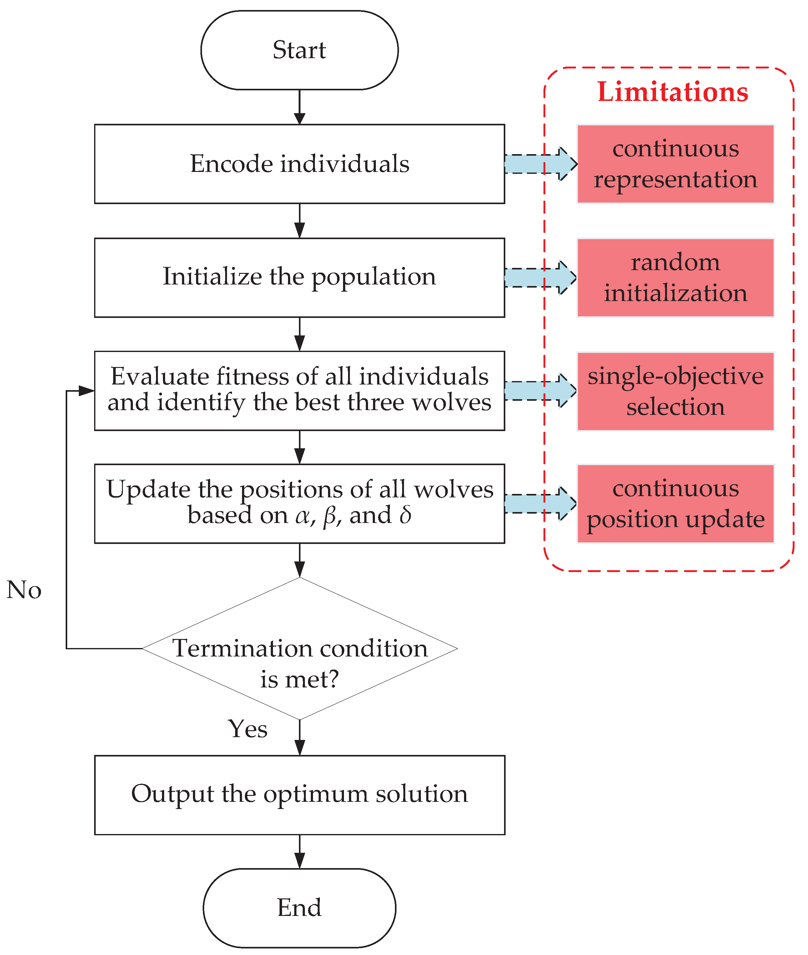
5.2. Original GWO and Its Limitations in Solving DFJSSP

GWO is a novel swarm intelligence optimization algorithm inspired by the hierarchical and hunting mechanism of gray wolf packs [49]. Each wolf in the pack represents a solution to the original optimization. During each iteration, all individuals in the wolf pack are categorized into four classes based on their fitness values to simulate the social hierarchy of the pack. The three wolves with the best fitness values, sequentially defined as α , β , and  δ , can guide other wolves, while all remaining wolves are classified as ω . The algorithm assumes that α , β , and  δ wolves can guide other wolves to locate and approach prey. Therefore, the positions of these three optimal wolves are preserved to direct the ω wolves’ predatory behavior. Through continuous iterations, the pack ultimately achieves the goal of capturing the prey. This process is represented as follows:
D α = | C 1 X α ( t ) X ( t ) | , D β = | C 2 X β ( t ) X ( t ) | , D δ = | C 3 X δ ( t ) X ( t ) | ,
X 1 = X α ( t ) A 1 D α , X 2 = X β ( t ) A 2 D β , X 3 = X δ ( t ) A 3 D δ ,
X ( t + 1 ) = X 1 + X 2 + X 3 3
where t indicates the current iteration, A and C are coefficient vectors, and X ( t + 1 ) denotes the position vector of each wolf in t. X α ( t ) , X β ( t ) , and X δ ( t ) denote the three best solutions found so far.
To further illustrate the fundamental process and working mechanism of GWO, a standard flowchart of the original GWO model is presented in Figure 2. As shown in the figure, GWO was originally developed for continuous single-objective optimization problems, and its standard workflow consists of continuous solution encoding, random population initialization, position updating based on continuous mathematical operations, and iterative global best solution refinement.
However, when applied to discrete multi-objective optimization problems, particularly the MODDFJSP, GWO exhibits several critical limitations. These can be broadly categorized into two dimensions: continuous vs. discrete representation and single-objective vs. multi-objective frameworks.
(1) Limitations related to continuous representation
Incompatible encoding and search space: The original GWO model employs continuous encoding and position updating mechanisms, which are not suitable for discrete and combinatorial solution representations required in scheduling problems, such as operation sequences or machine assignments.
Ineffective search operators: The use of continuous position updates in a discrete combinatorial search space leads to ineffective and infeasible exploration and exploitation, resulting in poor solution quality and premature convergence.
(2) Limitations related to single-objective framework
Lack of multi-objective support: The original GWO model is designed for single-objective optimization and thus lacks the ability to simultaneously consider and balance multiple conflicting objectives, such as makespan, tardiness, stability, and maximum factory load.
Random initialization: The standard random initialization strategy is not guided by problem-specific knowledge, leading to low-quality initial solutions and insufficient population diversity in multi-objective contexts.

5.3. Framework of the Proposed DIGWO

This study develops a DIGWO model tailored for the characteristics of the MODDFJSP. To provide a clear overview of the algorithm’s working process and its integration of various discrete and multi-objective mechanisms, the overall framwork of DIGWO is illustrated in Figure 3. The framework incorporates multiple modules. Each component is designed to address the limitations of the original GWO model in discrete and multi-objective contexts.
We further depict the framework of the proposed DIGWO as Algorithm 1. First, a set of N reference points are generated by using the uniform design method in [50]. Next, an initial population, P 0 , with N members is produced by using a problem-specific initialization strategy. The nondominated solutions in P 0 are obtained to construct the initial external archive Ω . Lines 6–24 are iterated until the termination criterion is satisfied. In each generation, t, in line 9, the three leading wolf packs are obtained by selecting a number of individuals from the external archive and first two nondomination levels. Then, for each wolf (solution), S t , in population, the leading wolves S α , S β , and  S δ are randomly selected from the three leading wolf packs, respectively. In line 13, the crossover operations are first performed to produce the offspring. After that, the mutation is performed with a certain probability, P m , to avoid stagnation in local optima. In lines 20–21, the new population P n e w ( t ) is merged with P ( t ) , and the best N wolves are selected as the next population P ( t + 1 ) from the merged population; this is achieved using fast nondominated sorting and a reference point-based selection mechanism proposed by Deb and Jain [51]. Finally, the external archive is updated. The pseudocode of Algorithm 1 is presented as follows.
Algorithm 1 Pseudocode of DIGWO.
  1:
Generate reference points Λ
  2:
Encode each individual by discrete integer encoding (see Section 5.4.1 for details)
  3:
Initialize a wolf group P 0 (see Section 5.4.2 for details)
  4:
Ω GetNondominatedSolutions( P 0 )
  5:
t 0
  6:
while stop criterion is not satisfied do
  7:
       P n e w ( t )
  8:
      // Multi-objective-based leader wolf packs selection mechanism
  9:
      Obtain the leader wolf packs by combining external archive with nondominated sorting (see Section 5.4.3 for details)
10:
      for each wolf S t P ( t )  do
11:
           Determine S α , S β , S δ from leader wolf packs and denote them as S l e a d e r
12:
           // Discrete search operators for the grey
13:
           o f f Cossover( S t , S l e a d e r ) (see Section 5.4.4 for details)
14:
          if  r a n d ( ) < P m  then
15:
              o f f Mutation( o f f ) (see Section 5.4.4 for details)
16:
          end if
17:
           P n e w ( t ) P n e w ( t ) o f f
18:
     end for
19:
      // Multi-objective selection mechanism
20:
      { F 1 , F 2 , , F l a s t } FastNondominatedSort( P ( t ) P n e w ( t ) )
21:
      P ( t + 1 ) ← EnviromentalSelection( F 1 , F 2 ,…, F l a s t )
22:
      Ω ← UpdateArchive( F 1 Ω ) (see Section 5.4.5 for details)
23:
      t t + 1
24:
 end while

5.4. The Improvements Introduced in DIGWO

To overcome the limitations of GWO listed in Section 5.2, the key improvements made in DIGWO are grouped into two major categories:
1. Enhancements for discrete operation
(1) A discrete integer encoding scheme and corresponding decoding method are employed to represent scheduling effectively in a combinatorial domain.
(2) Customized discrete crossover and mutation operators are used to replace continuous position updates, ensuring compatibility with the discrete nature of the problem.
2. Enhancements for multi-objective optimization
(1) A problem-specific population initialization strategy is adopted, combining multiple scheduling heuristics with dynamic features to generate diverse and high-quality initial solutions suited for multi-objective scheduling aspects.
(2) An external archive is introduced to retain nondominated solutions and guide the search process within a multi-objective framework.
(3) A multi-objective-based leader wolf pack selection mechanism is proposed to dynamic determine leadership hierarchy based on Pareto dominance and historical performance.
(4) A multi-objective environment selection mechanism is adopted, which combines nondominated sorting and reference-point association to select the next generation of solutions. This approach ensures convergence toward the Pareto front while maintaining a well-distributed solution set across the objective space.
The details of these modifications are elaborated in the subsequent sections.

5.4.1. Discrete Encoding Scheme and Corresponding Decoding Method

Currently, two mainstream approaches exist for adapting meta-heuristics to discrete scheduling problems [52]. The first approach employs continuous encoding and utilizes a transformation mechanism to map continuous position vectors to discrete scheduling solutions. Its main advantage lies in the simplicity of implementation and the ability to retain the original continuous position update framework. However, this transformation often results in precision loss, the omission of potentially high-quality solutions, and significant computational overhead. The second approach directly adopts a discrete encoding scheme, which better aligns with the combinatorial nature of scheduling problems and avoids the need for continuous-to-discrete mapping. Nevertheless, it cannot directly utilize traditional continuous position update strategies, limiting its search capability.
Considering the attributes of dynamic scheduling, high computational complexity affects the efficiency of scheduling methods and their timely response to dynamic events, this study adopts the second approach by introducing a discrete three-layer encoding method. This method includes factory assignment (FA), operation sequencing (OS), and machine selection (MS), corresponding well to three subproblems in the DFJSP. Take Table 2 as an example. Suppose that, at a specific rescheduling point, O 45 , O 53 , O 54 , O 55 , O 63 , O 64 , and O 78 are the operations, respectively, from J 4 , J 5 , J 6 , and J 7 ; these are left unprocessed in the previous schedule. Then, O 81 , O 82 , O 83 , O 91 , and O 92 are the operations from two new arrived jobs, J 8 and J 9 . Considering that the machine M 12 is a faulty machine, Figure 4 represents a possible solution encoding for the problem shown in Table 2. In the FA, the first gene value “2” indicates that the first job J 4 is assigned to U 2 for processing. In the OS, the first gene value “5” denotes that the first unprocessed operation of J 5 , i.e., O 53 . In the MS, the first gene value “2” indicates that the operation O 41 is assigned to the second machine in U 2 for processing. It can also be seen that J 8 and J 9 are assigned to the factories U 1 and U 2 , respectively, and the operation sequencing is interpreted as O 53 O 81 O 45 O 54 O 78 O 91 O 82 O 63 O 92 O 64 O 83 O 55 .
During the decoding process, the jobs are firstly assigned to corresponding factories in view of the FA. After that, each factory can be treated as an FJSP. Consequently, the insertion-based method proposed by Zhang et al. [53] is adopted to generate an active schedule. This approach ensures that each operation starts processing as early as possible. The schedule solution obtained using this method is also shown in Figure 5.

5.4.2. Problem-Specific Population Initialization Strategy

To improve the quality and diversity of the initial population in a multi-objective optimization context, we propose a problem-specific initialization strategy combining a dynamic-event-based heuristic approach with hybrid scheduling rules, with respective proportions of 40% and 60%. Specifically, the dynamic-event-based heuristic strategy maintains the workshop stability through local adjustments to the original schedule; meanwhile, the hybrid rules improve the robustness and diversity of initial solutions by adopting the mixed rules to initialize the three layers of each solution. Detailed explanations of these two methods are presented below:
(1) Dynamic-event-based heuristic approach
If there are machines that have been repaired in the last rescheduling interval, they should be added to the set of candidate machines for the corresponding operation first; according to different scenarios, the following heuristic strategies are performed.
As for machine breakdowns, all unaffected operations keep their original processing machines and start times. The directly affected operations, which are assigned to the faulty machines and not yet processed, are reassigned to other available machines. Here, the recently repaired machines might be preferable. Note that if a job cannot be processed within the current factory due to the machine breakdown, and the first operation has not begun, then the job is transferred to another factory. The indirectly affected operations retain their original machines but may have their processing sequence adjusted.
As for urgent job arrivals or period rescheduling, half of the jobs prioritize factories with fewer assigned operations. If two or more factories under the same conditions are available, then one factory is randomly selected. The other half of the jobs select factories at random. The jobs that have been assigned to the factories should be inserted into the machines in order of weight priority. With the aim of ensuring stability, for each operation, a gap insertion is performed on all available processing machines; here, it is preferable that the machine that can complete the operation at the earliest possible time is chosen.
(2) Hybrid scheduling rules
For the FA, we use the least job allocation rule and the random rule to generate individuals. The former gives preference to factories with the least allocated jobs in order to realize the workload balancing of factories; meanwhile, the latter assigns jobs to factories at random. The generated individuals are half composed of rule 1 and half composed of rule 2.
For the OS, we use most remaining operations, with the highest job weight and random rules to generate operation sequences for individuals. In the first rule, the job with the most remaining unprocessed operations is prioritized for selection. The specific implementation steps of the second rule are as follows: Randomly select five operations from all unsorted available operations to form a operation set. Then, select the operation with the highest job weight from the temporary set. If the number of operations is less than five, then the temporary set consists of all the remaining operations. The random rule generates an OS at random. The initial operation sequences are generated as follows: 30% of the solutions in the population are generated by rule 1, 30% of the solutions in the population are generated by rule 2, and the rest of the solutions in the population are generated by rule 3.
For the MS, we use the lowest operation allocation, the shortest processing time rule, and the random rule, comprising proportions of 30%, 30%, and 40%, to generate the initial machine assignments.

5.4.3. Multi-Objective-Based Leader Wolf Pack Selection Mechanism

In multi-objective optimization, the optimal solution is usually composed of a set of nondominated solutions. Therefore, traditional wolf pack partitioning methods that only guide population searches through three elite solutions may lead to premature convergence and reduce population diversity. Moreover, an external archive is used to store nondominated solutions that are found during the search in DIGWO. As a result, in this study, the wolf population is partitioned into different wolf packs by adopting a novel social hierarchy based on external archive and nondomination levels, and the detailed implementation is as follows: First, S α is selected from the external archive to ensure that the solution has good convergence. Next, if the population only contains one nondomination level, then S β and S δ are randomly selected from it. If the number of nondomination levels is more than one, then S β and S δ are selected from the first two nondomination levels, respectively.
Another difference from traditional GWO is that each wolf, S, randomly chooses its leading wolf according to different situations rather than sharing the same ones in each generation. If the wolf S belongs to the first nondomination level, then only S α and S β are selected as the leading wolves to conduct a crossover-based prey search in the following way:
o f f = Crossover ( S α , S ) , if r a n d < 0.5 Crossover ( S β , S ) , otherwise ,
if the wolf S is at the second nondomination level or worse, then S α , S β , and S δ are selected as the leading wolves, and the prey search can be represented as follows:
o f f = Crossover ( S α , S ) , if r a n d < 1 / 3 Crossover ( S β , S ) , if 1 / 3 r a n d < 2 / 3 Crossover ( S δ , S ) , otherwise .
Afterwards, in order to maintain the diversity of the population and enhance the local search ability, mutation is performed on each newly generated wolf with a certain probability. Details on crossover and mutation are described in later sections.

5.4.4. Discrete Search Operators for GWO

In accordance with the previously defined three-layer discrete encoding structure, traditional continuous position updating methods in GWO are no longer applicable. Therefore, this study adopts discrete position update strategies by designing customized crossover and mutation operators corresponding to each encoding layer. These operators enable effective solution evolution in the combinatorial space while preserving the structural integrity of the FA-OS-MS encoding.
Both crossover and mutation consist of three parts, in line with the three-layer encoding mechanism of each chromosome. However, crossover is applied to a pair of chromosomes, while mutation is applied to a single one. With regard to crossover, the FA part uses single-point crossover; that is, it randomly selects a position and swaps its corresponding elements. Improved precedence operation crossover (IPOX) [54] is utilized for OS. In IPOX, the job set is randomly divided into two sets, J S 1 and J S 2 . The elements of the first parent chromosome belonging to J S 1 are appended to the same position in the child chromosome and the elements of the second parent chromosome belonging to J S 2 are appended to the empty positions in the child chromosome, seriatim. For MS, the uniform crossover [55] is adopted. In uniform crossover, a binary string, which comprises the integers 0 and 1, is generated with the same length of two parent chromosomes. Then, the elements in the two parent chromosomes at a position with 1 in the binary string are exchanged in turn. Finally, the rest of the elements in the same position are copied to their offspring. It is worth noting that both the crossovers for FA and MS may make the MS part unfeasible. To address this issue, we adopt a repair strategy by randomly selecting a machine from the available machine set to replace the illegal one. The schematic of IPOX and uniform crossover are, respectively, shown in Figure 6 and Figure 7.
Mutation is performed to maintain the population diversity. As for FA, the single-point mutation is used; that is, a position is randomly selected and the elements are replaced by other factory numbers. For MS, this is achieved by changing the machine assignment of two operations that are chosen arbitrarily. As for OS, swap mutation [53] is adopted.

5.4.5. External Archive Update Strategy

To effectively preserve high-quality historical solutions during the optimization process, an external archive update mechanism is integrated into the proposed DIGWO. Designed within a multi-objective optimization framework, the external archive stores high-quality non-dominated solutions identified throughout the iterative search.
In each generation, nondominated solutions from the hybrid population are added to the external archive, Ω , and the nondominated solutions are recalculated from Ω . If the number of nondominated solutions exceeds the pre-set size of the external archive, then the reference-point-based selection mechanism in NSGA-III [51] is used to limit the archive size. Specifically, each nondominated solution in the external archive should first be associated with its nearest reference point. Then, the individuals corresponding to the reference points with the most associated solutions should be randomly deleted until the archive size meets the requirements. This external archive update strategy effectively controls the size of the external archive and ensures the distribution of solutions by combining nondominated solution updating and reference point association mechanisms.

6. Experiment and Analysis

This section is dedicated to systematically validating the effectiveness of the proposed DIGWO-based predictive–reactive method in the following five aspects: (1) Comparison to classical MOEAs; (2) Comparison to the complete reactive-based method; (3) Effectiveness analysis of the population initialization strategy; (4) Investigation of the trade-off relationship between each pair of the four concerned objectives; (5) Investigation of the impact of different rescheduling cycles. In the following section, we present an experimental preparation, containing the simulation of a distributed flexible job shop and dynamic events, parameter settings, and performance metrics. Then, we describe how extensive comparative experiments were carried out in a stage-by-stage manner to compare DIGWO-based predictive–reactive methods with other scheduling methods. Finally, the superiority of our proposed method is discussed.
The proposed method was implemented in MATLAB 2016b and ran on an Intel Core i7 @ 2.90GHz computer with 16GB of RAM.

6.1. Experimental Environments

To validate the effectiveness of the proposed method, a realistic distributed flexible job shop was simulated based on the simulator in [56] to simultaneously consider random job arrivals and machine breakdowns. Based on the parameters and relevant data provided in Table 3 and Equations (24) and (25), we simulated random job arrival; using Equations (26)–(29), we simulated machine breakdowns and repairs.
T B J A i = e x p r a n d ( M T B J A ) , i = 1 , 2 , ,
a i = T B J A i + a i 1 , i > 1 T B J A i , i = 1 ,
T B F k = e x p r a n d ( M T B F ) , k = 1 , 2 , , m ,
m t k = T B F k + m a k , k = 1 , 2 , , m ,
T T R k = e x p r a n d ( M T T R ) , k = 1 , 2 , , m ,
m a k = T T R k + m t k , k = 1 , 2 , , m ,
where a i denotes the arrival time of the job i; m t k and m a k denote the breakdown and available time of the machine k, respectively. The mean time between job arrivals ( M T B J A ) in Equation (24) can be calculated as follows:
M T B J A = A v g P A v g n u M ,
A v g P = i = 1 n j = 1 n i A v e r a g e P i j i = 1 n n i ,
A v g n = i = 1 n n i n ,
where A v g P represents the average processing time of all operations, A v g n denotes the average number of operations for the jobs, and M is the total number of machines in all factories.
The simulation model contained 360 jobs that needed to be processed by two factories. Among them, 10 jobs were present in the initial distributed flexible job shop; the simulation continued until the remaining 350 jobs arrived at the shop floor. In addition, the proportions of the three types of job weights were set to 60%, 30%, and 10%. One dynamic distributed flexible job shop instance was generated using the parameters introduced in Table 3; this was used as the problem instance in all the following experiments.

6.2. Other Algorithms in Comparsion

6.2.1. MOEAs for Comparsion

To comprehensively evaluate the effectiveness of the proposed DIGWO, the DIGWO was compared with three well-known MOEAs, namely NSGA-II [13], SPEA2 [14], and MOEA/D [15]. The reasons for selecting these three algorithms can be summarized as follows: (1) All of them are based on a framework stemming from GA, which is very suitable for solving various combinatorial optimization problems. (2) All of them are classical algorithms which are widely used for solving multi-objective optimization problems, and their effectiveness in different types of multi-objective scheduling problems has been well validated. (3) NSGA-II, SPEA2, and our DIGWO use the Pareto-dominance-based approach for dealing with the multiple objectives; meanwhile, MOEA/D adopts a decomposition strategy, providing a different optimization paradigm for comparison. To apply these three algorithms to solve MODDFJSPs and to ensure a fair comparison, all compared algorithms were implemented with the same discrete encoding scheme, decoding, crossover, mutation, and initialization methods. The parameter settings of these algorithms are listed in Table 4.

6.2.2. Variation of DIGWO for Comparsion

In addition to the main algorithm, DIGWO, a variant named DIGWOrand is introduced. DIGWOrand differs from DIGWO only in the initialization phase, where the initial population is generated randomly instead of using the proposed initialization strategy. All other algorithmic steps remain the same. This variant is designed to verify the effectiveness and contribution of the proposed initialization strategy by comparison. By comparing the performance of DIGWO with DIGWOrand, the impact of the proposed initialization strategy on solution quality and convergence can be clearly demonstrated.

6.3. Performance Metrics

Three quality indicators (hyper-volume (HV) [57], inverted generational distance (IGD) [58], and C-metric [59]) are adopted to evaluate the performance of the concerned algorithms. Detailed description of these are given here:
(1) Hyper-volume (HV)—Let A denote the final nondominated solution set of an algorithm in the objective space; r = ( r 1 , r 2 , , r M ) T is the reference point in the objective space which is dominated by any solution in the set A . HV( A , r ) measures the volume of the hypercube surrounded by the solutions and the reference points and can be described as
HV ( A , r ) = volume f A [ f 1 , r 1 ] × × [ f M , r M ] .
(2) Inverted generational distance (IGD)—Let P be the true Pareto front; the IGD can be calculated as
IGD ( A , P ) = 1 | P | x P min y A d ( x , y ) ,
where d ( x , y ) means the Euclidean distance between the points x and y. Seeing that the true Pareto front is invariably unknown for the MODDFJSP, P is obtained by extracting the nondominated solutions from the merging of solutions found during all runs of all the compared algorithms.
Both HV and IGD are comprehensive performance evaluation metrics. A larger HV value means better quality; meanwhile, the smaller the IGD is, the better the algorithm performance is. In this study, these two metrics are computed based on the normalized objective values of the nondominated solutions, which can be acquired as follows:
f ˜ i ( x ) = ( f i ( x ) f i m i n ) ( f i m a x f i m i n ) , i = 1 , 2 , 3 , 4 ,
where f i m a x and f i m i n are the maximum and minimum values among all the solution sets in terms of the ith objective. Accordingly, the the reference point for calculating HV was set to ( 1.1 , 1.1 , 1.1 , 1.1 ) T . In addition, we calculated the HV using the Monte Carlo simulation proposed in [60]; 100,000 sampling points were utilized to ensure the accuracy.
(3) C-metric—the C metric is used to compare the dominance of the nondominated solution sets of the two algorithms. Let A and B be two approximate Pareto sets; C ( A , B ) represents the percentage of solutions in B that are dominated by at least one solution in A and can be expressed as follows:
C ( A , B ) = b B | a A : a b | B | .
Obviously, if C ( A , B ) > C ( B , A ) , then A is better than B in a sense. However, it should be noted that C ( B , A ) is not equal to 1 C ( A , B ) .

6.4. Results and Discussion

6.4.1. Performance Comparison in the Whole Dynamic Scheduling Process

This section discusses in detail a performance comparison that was conducted among different algorithms throughout the entire dynamic scheduling process; there were 94 rescheduling points here. At each rescheduling point, all the algorithms listed in Table 4 were independently run 20 times. As for each metric, the Wilcoxon signed-rank [61] test with a significance level of 0.05 was carried out to size up the significant differences in the results obtained using all the compared algorithms. Table 5 summarizes the significance tests of DIGWO and other algorithms on HV, IGD, and C metrics at all 94 rescheduling points. In this table, “B”(“W”) means the number of rescheduling points at which the results of DIGWO are significantly better (worse) than those of other algorithms, and “E” means that no statistical difference is presented for DIGWO or the other algorithms. We further employed performance score metrics [62] to provide a more intuitive comparison.
Since the value reflects the number of other algorithms that significantly outperformed the corresponding algorithm in terms of the considered rescheduling points, algorithms with a smaller value performed better. In Figure 8, the performance score of each algorithm along with each rescheduling point is represented, and the average performance scores over all 94 rescheduling points for the five competitive algorithms are summarized in Figure 9, in which the overall rank of each algorithm on the basis of the score is also presented in the corresponding bracket.
Based on the above results, we can make some observations, outlined as follows:
(1)
DIGWO significantly outperformed DIGWOrand at 46 out of the 94 rescheduling points for HV and IGD and at 35 rescheduling points out of 94 for the C metric; meanwhile, DIGWOrand significantly outperformed DIGWO at only one point for HV and at two points for IGD and C. This demonstrates the effectiveness of the proposed initialization method well.
(2)
DIGWO was the best among all the compared algorithms. It can be seen that, when compared with any other algorithms, DIGWO obtained better values for HV, IGD, and C at more rescheduling points. Meanwhile, DIGWO had the best average performance score.
(3)
SPEA2 demonstrated competitiveness to some extent and obtained the second best average performance score. Specially for HV, it can be seen that the number of rescheduling points where SPEA2 was significantly better than DIGWO was only one less than the number of rescheduling points where DIGWO was significantly better than SPEA2. However, for the IGD and C metrics, DIGWO had a significant advantage over SPEA2.
(4)
MOEA/D had the worst performance among all algorithms because it obtained the worst performance scores at almost all the rescheduling points. In conclusion, Pareto domination is more suitable than the decomposition technique for solving MODDFJSP.
Additionally, we also calculate the performance values across rescheduling points to evaluate the overall algorithm performance from another perspective. For each algorithm, first, the average metric values for each run over all rescheduling points were obtained. Then, 20 of these values could be spontaneously acquired after 20 runs. Afterwards, the 20 mean values were averaged likewise, and the consequential mean standard deviation across rescheduling points was obtained using the following equation [42]
s t d * = i = 1 N R s t d i 2 N R ,
where N R denotes the number of runs; s t d i means the standard deviation across rescheduling points in the ith run. Table 6 and Table 7 show the average performance obtained using all the algorithms in terms of the entire dynamic scheduling process. The best values in Table 6 are marked in bold. The signs ‘+/−/=’ are for the related metrics: + means that DIGWO is significantly better than the compared algorithm; − means that DIGWO is worse than the compared algorithm; and = means that there is no significant difference between DIGWO and the compared algorithms. These assessments were determined according to the Wilcoxon signed-rank test. In addition, the values in Table 7 that are significantly better than the others are also marked in bold. It can be seen from these two tables that DIGWO performed best in terms of IGD and C. As for HV, although there exists no difference between DIGWO and SPEA2, DIGWO is better than the other algorithms.
The mean CPU time (in seconds) of the four compared algorithms at each rescheduling points is shown in Figure 10. It is clearly indicated from this figure that MOEA/D exhibited the lowest average CPU time since it optimized the subproblems in parallel and approached the Pareto front via aggregation function-based selection operation. In addition, DIGWO was more computationally expensive other algorithms, owing to the use of nondominated sorting and specific external archive maintenance strategies. However, it was still within an acceptable range.
Based on the extensive experimental results provided in this section, it can be concluded that DIGWO outperforms all the compared algorithms, and it is more suitable for solving the discussed problems. The main reasons for this are summarized here: Firstly, an effective social hierarchy is constructed based on the Pareto dominance relationship, which can ensure the rationality of wolf population partition in the sense of multi-objective optimization. Secondly, the external archive is designed to preserve nondominated solutions and to provide lead wolf pack—this not only prevents the loss of the optimal solutions but also enables the exploration of more promising regions within the solution space to enhance search efficiency. Thirdly, the elitist is implemented to select solutions from the merged population of each generation with the aim of accelerating convergence. Last but not least, DIGWO adoptes a reference-point-based environmental selection mechanism, which is more useful than nearest neighbor density and crowding distance in maintaining a solution distribution in many-objective problems (the number of objectives is more than three).

6.4.2. Performance Comparisons to Existing Dynamic Scheduling Methods

To validate the performance of the proposed DIGWO-based rescheduling method, we compared it with the performances of rule-based, completely reactive scheduling methods. Considering the fact that a DFJSP contains three subproblems—i.e., factory assignment, machine selection, and operation sequencing—rules corresponding to these three subproblems were designed respectively. At each rescheduling point, the jobs are first assigned to different factories according to a specific factory assignment rule. Then, for each factory that can be treated as an FJSP, the operations are assigned to different machines on the basis of the specific machine assignment rule; the operations remaining in the waiting queue are chosen on the basis of the priority dispatching rule—that is, the one with the highest priority will be processed once its corresponding machine becomes available.
At each rescheduling point, if new jobs arrive following the previous rescheduling point, two factory assignment rules are considered for assigning these new jobs. The first one finds the factory with the most unprocessed operations. Another one chooses the factories for each job at random. We call them FAR1 and FAR2. As for all available operations, which are derived from newly arrival jobs, some previously unavailable operations become available again due to the machine repairs and so on; we consider three machine assignments rules. The first one selects the machine with the shortest processing time from the current candidate machine set. The second one focus on selecting the machine with a minimal workload. The last one randomly select a machine for each operation. We call them MAR1, MAR2, and MAR3 for short. With regard to priority dispatching rules, three classical rules, namely short processing time (SPT), First-In-First-Out (FIFO), and Last-In-First-Out (LIFO), are employed.
Thus, in all, there are two factory assignment rules, three machine assignment rules, and three operation sequencing rules, making a total number of 18 rule combinations. Because complete reactive scheduling focus on making local scheduling decisions at specific times, the statistical comparison—just like that in the previous section—seems to be impossible to conduct between combination rules and DIGWO. Thus, 20 independent runs were replicated for each combination and DIGWO, and the results of average makespan, weighted average job tardiness, and average factory load during the whole running process of the distributed flexible job shop are listed in Table 8. The values highlighted in bold indicate the optimal results among the compared results. It can be clearly seen that, for the three objectives, the values obtained uisng DIGWO were better than the majority of the combination rules, especially for makespan and tardiness. However, it is interesting to note that, when using combination rules which contained the MAR1 rule, the factory loads obtained were smaller than those obtained using DIGWO. This is primarily because the MAR1 rule assigns each operation to the machine with SPT within its available machine set. While this approach ensures optimal factory load, it may lead to an excessive accumulation of pending operators on certain machines. Consequently, prolonged waiting times for processing can negatively impact both makespan and tardiness. Based on the analysis of the above results, it can be concluded that the DIGWO-based rescheduling method is more effective than combination rules-based scheduling methods, especially with regard to improving the indicators related to distributed workshop efficiency.

6.4.3. Further Discussion

In this section, we discuss two issues further. The first one is the trade-off between the concerned objectives; the other one is the influence of different rescheduling cycles, Δ T , on the distributed workshop performance.
Figure 11 exhibits the trade-off relationship between two of the four concerned objectives at one specific rescheduling point by listing the nondominated solutions in a 2D plot from the combination of evolved Pareto fronts with respect to each run of each algorithm. In general, there is clear conflict between stability and the other three objectives (makespan, tardiness, and maximal factory load). There is almost no conflict between makespan, tardiness, and maximal factory load. This is because a shorter makespan requires the full utilization of all manufacturing resources to complete the processing of all jobs as soon as possible, which promotes load balancing across different factories. Moreover, a reduced completion time implies that jobs can be delivered to customers earlier, thereby minimizing the likelihood of delays. It is of great importance that DIGWO can effectively generate a set of nondominated solutions for the shop manger to understand the trade-offs among different objectives and make an informed decision in dynamic scheduling.
To investigate the impact of different rescheduling cycles, Δ T , we set four distinct values of 6, 12, 24, and 48 and the three objectives shown in Table 8 were considered. Each configuration was independently executed 10 times, and the average values of the three objectives were calculated. It can be seen from Figure 12 that different settings of Δ T had certain impacts on all three objectives. Firstly, the best makespan and job tardiness and the second best mean factory load were obtained when Δ T is 12, which indicates that the value of 12 is suitable for the dynamic scheduling problem in this study. Secondly, when the rescheduling cycle took the minimum value, all three objective values deteriorated, which means that increasing the periodic scheduling times may not necessarily improve scheduling performance. Finally, we can see that reducing the frequency of periodic scheduling can improve the average factory load to some extent, but it is not useful for the completion time and delay of workpieces. Therefore, it is crucial to set a reasonable rescheduling cycle value.

7. Conclusions

In this paper, a DFJSP with random job arrivals and machine breakdowns was studied. With the aim of capturing the dynamic and multi-objective nature of such a problem, a DIGWO-based predictive–reactive scheduling method was proposed. A dynamic periodic- and event-driven scheduling strategy was developed by triggering rescheduling to respond to dynamic events. A static scheduling window was constructed according to the updated factory and workshop state at each rescheduling point, and a mathematical model of an MODDFJSP was established by simultaneously considering makespan, weighted job tardiness, maximal factory load, and stability. Moreover, DIGWO with effective population initialization, prey search, and an external archive mechanism was designed to generate a set of trade-off solutions; these are beneficial in aiding shop managers in making an informed decision.
In the experiment phase, first, DIGWO was compared with its variant, and the results demonstrated that the hybrid initialization strategies could effectively improve its convergence. Then, extensive comparisons were conducted between DIGWO and three well-known MOEA-based predictive–reactive methods (NSGA-II, SPEA2, and MOEA/D). According to the statistical results based on three classical performance indicators (HV, IGD, and C), the proposed DIGWO outperformed the other three algorithms and demonstrated a strong ability to search for better Pareto solutions of MODDFJSPs. Third, the DIGWO-based predictive–reactive method was compared with completely reactive scheduling methods, which were implemented by combining different factory assignment, machine assignment, and operation sequencing rules. The final comparison results indicate that our method achieved the best makespan, weighted average job tardiness, and average factory load by a considerable margin. Moreover, we analyzed the trade-offs between the objectives and found that stability conflicted with the other three objectives. Finally, further analysis was conducted on the impact of different rescheduling cycles, revealing that setting a reasonable cycle value is crucial.
The primary limitation of this work lies in the insufficiency of case studies. The research conclusions derived in this paper should be interpreted in conjunction with the distributed workshop system employed in the simulation analysis. However, real-world production involves diverse manufacturing resources and production tasks. Therefore, it is necessary to apply the proposed method to more varied distributed workshop production conditions and scenarios and conduct additional case studies to validate the applicability and generalizability of the approach.
In future work, more uncertainties in DFJSPs will be considered, such as the impact of a changing due date. In addition, it is important to study green DFJSPs by considering energy-consumption-related indictors.

Author Contributions

Conceptualization, C.W. and J.C.; methodology, C.W. and J.C.; software, J.C.; validation, C.W. and B.X.; data curation, J.C.; writing—original draft preparation, C.W.; writing—review and editing, J.C. and S.L.; visualization, J.C. and S.L.; supervision, C.W. and B.X.; funding acquisition, C.W. and B.X. All authors have read and agreed to the published version of the manuscript.

Funding

This research was funded by the National Natural Science Foundation of China (Grant No. 62006092), the Natural Science Research Project of Anhui Educational Committee (Grant No. 2023AH030081), the Young and Middle-aged Teachers Training Action Project of Anhui Province (Grant No. JNFX2023017), and the Science and Technology Project of Wuhu (Grant No. 2023jc05).

Data Availability Statement

Data are contained within the article.

Acknowledgments

The authors would like to thank the anonymous reviewers and the editor for their positive comments.

Conflicts of Interest

The authors declare no conflicts of interest.

Abbreviations

The following abbreviations are used in this manuscript:
FJSPFlexible Job Shop Scheduling Problem
DFJSPDistributed Flexible Job Shop Scheduling Problem
DDFJSPDynamic Distributed Flexible Job Shop Scheduling Problem
MODFJSPMulti-objective Distributed Flexible Job Shop Scheduling Problem
MODDFJSPMulti-objective Dynamic Distributed Flexible Job Shop Scheduling Problem
MOEA Multi-objective Evolutionary Algorithm
GAGenetic Algorithm
GWOGray Wolf Optimization Algorithm
DIGWODiscrete Improved Gray Wolf Optimization
NSGA-IINondominated Sorting Genetic Algorithm II

References

  1. Li, R.; Gong, W.; Wang, L.; Lu, C.; Zhuang, X. Surprisingly Popular-Based Adaptive Memetic Algorithm for Energy-Efficient Distributed Flexible Job Shop Scheduling. IEEE Trans. Cybern. 2023, 53, 8013–8023. [Google Scholar] [CrossRef] [PubMed]
  2. Zhang, Z.; Li, Y.; Qian, B.; Hu, R.; Yang, J. A multidimensional probabilistic model based evolutionary algorithm for the energy-efficient distributed flexible job-shop scheduling problem. Eng. Appl. Artif. Intell. 2024, 135, 108841. [Google Scholar] [CrossRef]
  3. Wang, J.; Han, H.; Wang, L. A Feedback Learning-Based Memetic Algorithm for Energy-Aware Distributed Flexible Job-Shop Scheduling with Transportation Constraints. IEEE Trans. Evol. Comput. 2024, 1. [Google Scholar] [CrossRef]
  4. Zhang, Z.; Yin, Y.; Fu, Y. An ensemble of brain storm optimization and Q-learning methods for distributed flexible job shop scheduling problems with distribution operations. Int. J. Gen. Syst. 2024, 53, 863–897. [Google Scholar] [CrossRef]
  5. Li, R.; Gong, W.; Wang, L.; Lu, C.; Jiang, S. Two-stage knowledge-driven evolutionary algorithm for distributed green flexible job shop scheduling with type-2 fuzzy processing time. Swarm Evol. Comput. 2022, 74, 101139. [Google Scholar] [CrossRef]
  6. Liu, Y.; As’arry, A.; Hassan, M.K.; Hairuddin, A.A.; Mohamad, H. Review of the grey wolf optimization algorithm: Variants and applications. Neural Comput. Appl. 2024, 36, 2713–2735. [Google Scholar] [CrossRef]
  7. Li, X.; Xie, J.; Ma, Q.; Gao, L.; Li, P. Improved gray wolf optimizer for distributed flexible job shop scheduling problem. Sci. China Technol. Sci. 2022, 65, 2105–2115. [Google Scholar] [CrossRef]
  8. Zhu, Z.; Zhou, X.; Cao, D.; Li, M. A shuffled cellular evolutionary grey wolf optimizer for flexible job shop scheduling problem with tree-structure job precedence constraints. Appl. Soft Comput. 2022, 125, 109235. [Google Scholar] [CrossRef]
  9. Wang, J.; Liu, Y.; Ren, S.; Wang, C.; Wang, W. Evolutionary game based real-time scheduling for energy-efficient distributed and flexible job shop. J. Clean. Prod. 2021, 293, 126093. [Google Scholar] [CrossRef]
  10. Zhu, K.; Gong, G.; Peng, N.; Zhang, L.; Huang, D.; Luo, Q.; Li, X. Dynamic distributed flexible job-shop scheduling problem considering operation inspection. Expert Syst. Appl. 2023, 224, 119840. [Google Scholar] [CrossRef]
  11. Zhang, H.; Qin, C.; Xu, G.; Chen, Y.; Gao, Z. An energy-saving distributed flexible job shop scheduling with machine breakdowns. Appl. Soft Comput. 2024, 167, 112276. [Google Scholar] [CrossRef]
  12. Zhu, N.; Gong, G.; Lu, D.; Huang, D.; Peng, N.; Qi, H. An effective reformative memetic algorithm for distributed flexible job-shop scheduling problem with order cancellation. Expert Syst. Appl. 2024, 237, 121205. [Google Scholar] [CrossRef]
  13. Deb, K.; Pratap, A.; Agarwal, S.; Meyarivan, T. A fast and elitist multiobjective genetic algorithm: NSGA-II. IEEE Trans. Evol. Comput. 2002, 6, 182–197. [Google Scholar] [CrossRef]
  14. Zitzler, E.; Laumanns, M.; Thiele, L. SPEA2: Improving the Strength Pareto Evolutionary Algorithm For Multiobjective Optimization. In Proceedings of the Evolutionary Methods for Design, Optimization and Control with Applications to Industrial Problems, EUROGEN’2001, Athens, Greece, 19–21 September 2001. [Google Scholar]
  15. Zhang, Q.; Li, H. MOEA/D: A Multiobjective Evolutionary Algorithm Based on Decomposition. IEEE Trans. Evol. Comput. 2007, 11, 712–731. [Google Scholar] [CrossRef]
  16. Chan, F.T.; Chung, S.; Chan, P. An adaptive genetic algorithm with dominated genes for distributed scheduling problems. Expert Syst. Appl. 2005, 29, 364–371. [Google Scholar] [CrossRef]
  17. De Giovanni, L.; Pezzella, F. An Improved Genetic Algorithm for the Distributed and Flexible Job-shop Scheduling problem. Eur. J. Oper. Res. 2010, 200, 395–408. [Google Scholar] [CrossRef]
  18. Ziaee, M. A heuristic algorithm for the distributed and flexible job-shop scheduling problem. J. Supercomput. 2014, 67, 69–83. [Google Scholar] [CrossRef]
  19. Xie, J.; Li, X.; Gao, L.; Gui, L. A hybrid genetic tabu search algorithm for distributed flexible job shop scheduling problems. J. Manuf. Syst. 2023, 71, 82–94. [Google Scholar] [CrossRef]
  20. Zhang, Z.; Fu, Y.; Gao, K.; Zhang, H.; Wang, L. A cooperative evolutionary algorithm with simulated annealing for integrated scheduling of distributed flexible job shops and distribution. Swarm Evol. Comput. 2024, 85, 101467. [Google Scholar] [CrossRef]
  21. Samhouri, M.; Qareish, S.Z. Hybrid fuzzy genetic algorithm for the integration of process planning and scheduling for distributed flexible job shop. Neural Comput. Appl. 2025, 37, 2775–2798. [Google Scholar] [CrossRef]
  22. Wang, C.; Wei, M.; Liu, Q.; Zhang, X.; Li, X. An improved adaptive hybrid algorithm for solving distributed flexible job shop scheduling problem. Swarm Evol. Comput. 2025, 94, 101873. [Google Scholar] [CrossRef]
  23. Du, Y.; Li, J.; Luo, C.; Meng, L. A hybrid estimation of distribution algorithm for distributed flexible job shop scheduling with crane transportations. Swarm Evol. Comput. 2021, 62, 100861. [Google Scholar] [CrossRef]
  24. Yu, F.; Lu, C.; Zhou, J.; Yin, L.; Wang, K. A knowledge-guided bi-population evolutionary algorithm for energy-efficient scheduling of distributed flexible job shop problem. Eng. Appl. Artif. Intell. 2024, 128, 107458. [Google Scholar] [CrossRef]
  25. Zhao, F.; Li, M.; Zhu, N.; Xu, T.; Jonrinaldi. Multi-objective fitness landscape-based estimation of distribution algorithm for distributed heterogeneous flexible job shop scheduling problem. Appl. Soft Comput. 2025, 171, 112780. [Google Scholar] [CrossRef]
  26. Yan, Q.; Wang, H.; Yang, S. A Learning-Assisted Bi-Population Evolutionary Algorithm for Distributed Flexible Job-Shop Scheduling with Maintenance Decisions. IEEE Trans. Evol. Comput. 2024, 1. [Google Scholar] [CrossRef]
  27. Deng, L.; Qiu, Y.; Di, Y.; Zhang, L. A knowledge-driven memetic algorithm for distributed green flexible job shop scheduling considering the endurance of machines. Appl. Soft Comput. 2025, 170, 112697. [Google Scholar] [CrossRef]
  28. Wu, X.; Liu, X.; Zhao, N. An improved differential evolution algorithm for solving a distributed assembly flexible job shop scheduling problem. Memetic Comput. 2019, 11, 335–355. [Google Scholar] [CrossRef]
  29. Du, B.; Han, S.; Guo, J.; Li, Y. A hybrid estimation of distribution algorithm for solving assembly flexible job shop scheduling in a distributed environment. Eng. Appl. Artif. Intell. 2024, 133, 108491. [Google Scholar] [CrossRef]
  30. Sang, Y.; Tan, J. Intelligent factory many-objective distributed flexible job shop collaborative scheduling method. Comput. Ind. Eng. 2022, 164, 107884. [Google Scholar] [CrossRef]
  31. Zadeh, M.S.; Katebi, Y.; Doniavi, A. A heuristic model for dynamic flexible job shop scheduling problem considering variable processing times. Int. J. Prod. Res. 2019, 57, 3020–3035. [Google Scholar] [CrossRef]
  32. Al-Hinai, N.; ElMekkawy, T. Robust and stable flexible job shop scheduling with random machine breakdowns using a hybrid genetic algorithm. Int. J. Prod. Econ. 2011, 132, 279–291. [Google Scholar] [CrossRef]
  33. Soofi, P.; Yazdani, M.; Amiri, M.; Adibi, M.A. Robust Fuzzy-Stochastic Programming Model and Meta-Heuristic Algorithms for Dual-Resource Constrained Flexible Job-Shop Scheduling Problem Under Machine Breakdown. IEEE Access 2021, 9, 155740–155762. [Google Scholar] [CrossRef]
  34. Duan, J.; Wang, J. Robust scheduling for flexible machining job shop subject to machine breakdowns and new job arrivals considering system reusability and task recurrence. Expert Syst. Appl. 2022, 203, 117489. [Google Scholar] [CrossRef]
  35. Shen, X.; Han, Y.; Fu, J. Robustness measures and robust scheduling for multi-objective stochastic flexible job shop scheduling problems. Soft Comput. 2017, 21, 6531–6554. [Google Scholar] [CrossRef]
  36. Luo, S.; Zhang, L.; Fan, Y. Dynamic multi-objective scheduling for flexible job shop by deep reinforcement learning. Comput. Ind. Eng. 2021, 159, 107489. [Google Scholar] [CrossRef]
  37. Wu, Z.; Fan, H.; Sun, Y.; Peng, M. Efficient Multi-Objective Optimization on Dynamic Flexible Job Shop Scheduling Using Deep Reinforcement Learning Approach. Processes 2023, 11, 2018. [Google Scholar] [CrossRef]
  38. Nguyen, S.; Mei, Y.; Zhang, M. Genetic programming for production scheduling: A survey with a unified framework. Complex Intell. Syst. 2017, 3, 41–66. [Google Scholar] [CrossRef]
  39. Ozturk, G.; Bahadir, O.; Teymourifar, A. Extracting priority rules for dynamic multi-objective flexible job shop scheduling problems using gene expression programming. Int. J. Prod. Res. 2019, 57, 3121–3137. [Google Scholar] [CrossRef]
  40. Zhang, Y.; Wang, J.; Liu, Y. Game theory based real-time multi-objective flexible job shop scheduling considering environmental impact. J. Clean. Prod. 2017, 167, 665–679. [Google Scholar] [CrossRef]
  41. Zhang, L.; Li, X.; Wen, L.; Zhang, G. An efficient memetic algorithm for dynamic flexible job shop scheduling with random job arrivals. Int. J. Softw. Sci. Comput. Intell. 2013, 5, 63–77. [Google Scholar] [CrossRef]
  42. Shen, X.N.; Yao, X. Mathematical modeling and multi-objective evolutionary algorithms applied to dynamic flexible job shop scheduling problems. Inf. Sci. 2015, 298, 198–224. [Google Scholar] [CrossRef]
  43. Xu, W.; Shao, L.; Yao, B.; Zhou, Z.; Pham, D.T. Perception data-driven optimization of manufacturing equipment service scheduling in sustainable manufacturing. J. Manuf. Syst. 2016, 41, 86–101. [Google Scholar] [CrossRef]
  44. Sreekara Reddy, M.; Ratnam, C.; Rajyalakshmi, G.; Manupati, V. An effective hybrid multi objective evolutionary algorithm for solving real time event in flexible job shop scheduling problem. Measurement 2018, 114, 78–90. [Google Scholar] [CrossRef]
  45. Komaki, G.; Kayvanfar, V. Grey Wolf Optimizer algorithm for the two-stage assembly flow shop scheduling problem with release time. J. Comput. Sci. 2015, 8, 109–120. [Google Scholar] [CrossRef]
  46. Jiang, T.; Zhang, C. Application of Grey Wolf Optimization for Solving Combinatorial Problems: Job Shop and Flexible Job Shop Scheduling Cases. IEEE Access 2018, 6, 26231–26240. [Google Scholar] [CrossRef]
  47. Zhang, W.; Zheng, Y.; Ahmad, R. An energy-efficient multi-objective scheduling for flexible job-shop-type remanufacturing system. J. Manuf. Syst. 2023, 66, 211–232. [Google Scholar] [CrossRef]
  48. Zhang, H.; Chen, Y.; Zhang, Y.; Xu, G. Energy-Saving Distributed Flexible Job Shop Scheduling Optimization with Dual Resource Constraints Based on Integrated Q-Learning Multi-Objective Grey Wolf Optimizer. Comput. Model. Eng. Sci. 2024, 140, 1459–1483. [Google Scholar] [CrossRef]
  49. Mirjalili, S.; Mirjalili, S.M.; Lewis, A. Grey Wolf Optimizer. Adv. Eng. Softw. 2014, 69, 46–61. [Google Scholar] [CrossRef]
  50. Tan, Y.; Jiao, Y.; Li, H.; Wang, X. MOEA/D + uniform design: A new version of MOEA/D for optimization problems with many objectives. Comput. Oper. Res. 2013, 40, 1648–1660. [Google Scholar] [CrossRef]
  51. Deb, K.; Jain, H. An Evolutionary Many-Objective Optimization Algorithm Using Reference-Point-Based Nondominated Sorting Approach, Part I: Solving Problems With Box Constraints. IEEE Trans. Evol. Comput. 2014, 18, 577–601. [Google Scholar] [CrossRef]
  52. Kong, X.; Yao, Y.; Yang, W.; Yang, Z.; Su, J. Solving the Flexible Job Shop Scheduling Problem Using a Discrete Improved Grey Wolf Optimization Algorithm. Machines 2022, 10, 1100. [Google Scholar] [CrossRef]
  53. Zhang, G.; Gao, L.; Shi, Y. An effective genetic algorithm for the flexible job-shop scheduling problem. Expert Syst. Appl. 2011, 38, 3563–3573. [Google Scholar] [CrossRef]
  54. Wang, X.; Gao, L.; Zhang, C.; Shao, X. A multi-objective genetic algorithm based on immune and entropy principle for flexible job-shop scheduling problem. Int. J. Adv. Manuf. Technol. 2010, 51, 757–767. [Google Scholar] [CrossRef]
  55. Wang, L.; Zhou, G.; Xu, Y.; Liu, M. An enhanced Pareto-based artificial bee colony algorithm for the multi-objective flexible job-shop scheduling. Int. J. Adv. Manuf. Technol. 2012, 60, 1111–1123. [Google Scholar] [CrossRef]
  56. Zhang, L.; Gao, L.; Li, X. A hybrid intelligent algorithm and rescheduling technique for job shop scheduling problems with disruptions. Int. J. Adv. Manuf. Technol. 2013, 65, 1141–1156. [Google Scholar] [CrossRef]
  57. Zitzler, E.; Thiele, L. Multiobjective evolutionary algorithms: A comparative case study and the strength Pareto approach. IEEE Trans. Evol. Comput. 1999, 3, 257–271. [Google Scholar] [CrossRef]
  58. Bosman, P.; Thierens, D. The balance between proximity and diversity in multiobjective evolutionary algorithms. IEEE Trans. Evol. Comput. 2003, 7, 174–188. [Google Scholar] [CrossRef]
  59. Zitzler, E.; Deb, K.; Thiele, L. Comparison of Multiobjective Evolutionary Algorithms: Empirical Results. Evol. Comput. 2000, 8, 173–195. [Google Scholar] [CrossRef]
  60. Bader, J.; Zitzler, E. HypE: An Algorithm for Fast Hypervolume-Based Many-Objective Optimization. Evol. Comput. 2011, 19, 45–76. [Google Scholar] [CrossRef]
  61. Demšar, J. Statistical Comparisons of Classifiers over Multiple Data Sets. J. Mach. Learn. Res. 2006, 7, 1–30. [Google Scholar]
  62. Yuan, Y.; Xu, H.; Wang, B.; Yao, X. A New Dominance Relation-Based Evolutionary Algorithm for Many-Objective Optimization. IEEE Trans. Evol. Comput. 2016, 20, 16–37. [Google Scholar] [CrossRef]
Figure 1. Flowchart of the predictive–reactive method.
Processes 13 01987 g001
Figure 2. Flowchart of GWO.
Processes 13 01987 g002
Figure 3. Flowchart of DIGWO.
Processes 13 01987 g003
Figure 4. An example of an encoding method.
Processes 13 01987 g004
Figure 5. An example of decoding.
Processes 13 01987 g005
Figure 6. The schematic of IPOX.
Processes 13 01987 g006
Figure 7. The schematic of uniform crossover.
Processes 13 01987 g007
Figure 8. Performance score along with each rescheduling point. The smaller the score is, the better the algorithm performed. (a) HV. (b) IGD.
Processes 13 01987 g008
Figure 9. Ranking of the average performance scores over all rescheduling points. The smaller the score is, the better the algorithm performed. (a) HV. (b) IGD.
Processes 13 01987 g009
Figure 10. CPU time comparison of four algorithms at each rescheduling point.
Processes 13 01987 g010
Figure 11. Pareto front of the non-dominated solutions plotted on two of the four objectives at one specific rescheduling point.
Processes 13 01987 g011
Figure 12. Examination of the influence of Δ T on three objectives.
Processes 13 01987 g012
Table 1. Notations.
Table 1. Notations.
t r the rescheduling point ( r = 1 , 2 , ) n ( t r ) the number of jobs which contain unprocessed and
available operations at t r
ithe index of jobs, i = 1 , 2 , , n ( t r ) fthe number of factories
lthe index of factories, l = 1 , 2 , , f U l the lth factory
m l ( t r ) the number of available machines in U l at t r M l k the kth available machine in U l
kthe index of available machines in U l J i ( t r ) the ith job at t r
q l k ( t r ) the number of operations that are assigned on M l k O l k a ( t r ) the ath operation that is processed on M l k
p l k a ( t r ) the processing time of O l k a ( t r ) jthe index of operations belonging to J i ( t r )
ω i the weight of J i ( t r ) C i ( t r ) the completion time of J i ( t r )
I i ( t r ) the index of the first unprocessed operation of J i ( t r ) n i ( t r ) the number of unprocessed and available opertaions
corresponding to J i ( t r )
D D i ( t r ) the due date of J i ( t r ) O i j ( t r ) the jth operation of J i ( t r ) ,
j = I i ( t r ) , I i ( t r ) + 1 , , I i ( t r ) + n i ( t r ) 1
s i j ( t r ) the starting time of O i j ( t r ) O * the set of unprocessed and available operations
which appear at both t r and t r 1
J * the set of jobs which contain unprocessed and
available operations at both t r and t r 1
z i l ( t r ) if J i ( t r ) is processed in U l , z i l ( t r ) = 1 ;
otherwise, z i l ( t r ) = 0
M l * the set of available machines in U l
which appear at both t r and t r 1
X i , j l , k ( t r ) if O i j ( t r ) is processed on M l k , X i , j l , k ( t r ) = 1 ;
otherwise, X i , j l , k ( t r ) = 0
a i the time when J i ( t r ) arrives at the distributed
workshop
K i the tightness factor which follows a normal
distribution with a mean of 1.5 and variance of 0.5
A v e r a g e P i j the average processing time of O i j ( t r ) β i if J i ( t r ) has already had an operation
processed at t r , β i = 1 ; otherwise, β i = 0
A v e r a g e P i j l the average processing time of O i j ( t r ) related to U l c i j ( t r ) the completion time of O i j ( t r )
M K A i j l ( t r ) the set of available machines in U l
that can process O i j ( t r ) at t r
p i j l k ( t r ) the processing time of O i j ( t r ) on M l k
R i ( t r ) the initial release time of J i ( t r ) C i ( I i ( t r 1 ) ) the completion time of the last operation of J i ( t r )
which is completed before t r
Y l k ( t r ) the initial available time of M l k c l , k l a s t ( t r 1 ) the completion time of the last operation
processed on M l k before t r
c O l k a ( t r ) the completion time of O l k a ( t r ) y i , j l , k , a ( t r ) if O i j ( t r ) is the ath operation processed on M l k
y i , j l , k , a ( t r ) = 1 ; otherwise, y i , j l , k , a ( t r ) = 0
Table 2. A case of a DDFJSP with six jobs and two factories at one specific rescheduling point.
JobInstance U 1 U 2
M 11 M 12 * M 13 M 21 M 22 M 23
J 4 O 45 347 74
J 5 O 53 4342
O 54 5533
O 55 24343
J 6 O 63 3457
O 64 12313
J 7 O 78 68455
J 8 O 81 57825
O 82 646758
O 83 1363
J 9 O 91 552324
O 92 24315
* means that the corresponding machine malfunctions at one specific rescheduling point. ★− means the machine cannot process the corresponding operation.
Table 3. Summary of the parameters used in the design of experiments.
CharacteristicsSpecifications
Distributed flexible job shop
Number of factories2
Number of machines in each factory, m8
Shop utilization, u0.8
Mean time between failures ( M T B F ) U [ 100 , 200 ] *
Mean time to repair ( M T T R ) U [ 20 , 80 ]
Time interval between failures ( T B F )Exponential distribution with mean of M T B F
Time to repair ( T T R )Exponential distribution with mean of M T T R
Jobs
Number of operations in each job U [ 1 , m ]
Number of candidate machines for each job U [ 1 , m ]
Time between new job arrivals ( T B J A )Exponential distribution with mean of M T B J A
Processing time of each opeartionExponential distribution with mean of 2
* U ( a , b ) denotes a number generated uniformly at random from the interval of [a,b].
Table 4. Parameter settings of all concerned algorithms.
ParameterDIGWONSGA-IISPEA2MOEA/D
Population size, N100100100100
Crossover probability*0.80.8
Mutation probability0.10.10.10.1
Neighborhood size, T0.1N
External archive sizesame as Nsame as Nsame as N
Number of runs20202020
Maximum number of objective evaluations20,00020,00020,00020,000
*—means that the corresponding parameters are not required.
Table 5. Summary of the significance test between DIGWO and the other algorithms.
NSGA-IISPEA2MOEA/D DIGWOrand
DIGWO vs.
(HV)
B36189146
W71701
E5159347
DIGWO vs.
(IGD)
B61429246
W0702
E3345246
DIGWO vs.
(C)
B22839235
W9302
E638257
Table 6. Comparisons of the average performances of five algorithms across rescheduling points in terms of HV and IGD.
Algorithm HVIGD
DIGWOMean1.0790.069
Std0.2310.041
NSGA-IIMean1.057(+)0.085(+)
Std0.2460.052
SPEA2Mean1.078(=)0.074(+)
Std0.2290.040
MOEA/DMean0.903(+)0.146(+)
Std0.2470.068
DIGWOrandMean1.054(+)0.077(+)
Std0.2350.044
Table 7. Comparisons of the average performances of five algorithms across rescheduling points in terms of C.
DIGWO(A)
vs.
NSGA-II(B)
DIGWO(A)
vs.
SPEA2(C)
DIGWO(A)
vs.
MOEA/D(D)
DIGWO(A)
vs.
DIGWOrand(E)
C(A,B) C(B,A) C(A,C) C(C,A) C(A,D) C(D,A) C(A,E) C(E,A)
Mean0.1960.1620.3500.1040.5920.1430.2690.158
Std0.1940.1760.2140.1340.3030.1810.2210.180
Table 8. Comparisons of the DIGWO-based rescheduling methods against the existing dynamic scheduling methods.
Scheduling MethodsMakespanWeighted Average Job TardinessAvg Factory Load
FAR1+MAR1+SPT570.7884.53901.00
FAR1+MAR2+SPT1122.50526.692018.63
FAR1+MAR3+SPT1175.85559.732049.72
FAR2+MAR1+SPT577.5788.41886.10
FAR2+MAR2+SPT1115.62520.962033.60
FAR2+MAR3+SPT1182.18546.122042.13
FAR1+MAR1+FIFO737.41180.09891.85
FAR1+MAR2+FIFO1374.00705.882042.89
FAR1+MAR3+FIFO1491.61784.762051.19
FAR2+MAR1+FIFO737.41177.12888.20
FAR2+MAR2+FIFO1391.53716.152050.48
FAR2+MAR3+FIFO1491.48792.412055.87
FAR1+MAR1+LIFO747.26186.82896.39
FAR1+MAR2+LIFO1425.64748.862038.31
FAR1+MAR3+LIFO1485.88794.632067.00
FAR2+MAR1+LIFO750.44178.68889.75
FAR2+MAR2+LIFO1402.42740.662045.95
FAR2+MAR3+LIFO1465.94782.292048.33
DIGWO440.0534.721022.46
Disclaimer/Publisher’s Note: The statements, opinions and data contained in all publications are solely those of the individual author(s) and contributor(s) and not of MDPI and/or the editor(s). MDPI and/or the editor(s) disclaim responsibility for any injury to people or property resulting from any ideas, methods, instructions or products referred to in the content.

