Abstract
In this study, using in-house code I-COSTA, importance analyses are performed on the phenomenological parameters in the aerosol dynamics using International Standard Problem No. 44. The analyses consider twelve parameters used in multicomponent sectional equations and Mason equations. For the first step of the analysis, Latin hypercube sampling is performed for the aforementioned parameters, and the number of samplings is determined using a comparison of averages and standard deviations between those samplings and the ones gathered from continuous distributions of the parameters. Sensitivity analyses are then performed on the airborne concentrations of the aerosol particles using I-COSTA, and the results are used to obtain the correlation coefficients between the parameters and the airborne concentrations. From the analyses, the dynamic shape factor, which accounts for the drag force of the non-spherical aerosol particles, is found to be one of the most important parameters in the aerosol dynamics. The saturation ratio in the Mason equation is also found to be an important parameter for aerosol particles with high solubility since the mass of the aforementioned particles is sensitive to the hygroscopic growth rate.
1. Introduction
The nuclear accident source term is one of the most important engineering values for safety analyses in nuclear engineering since it is used to determine how a nuclear power plant is designed to manage and mitigate accidents. The source term provides the initial and boundary conditions for the consequence analysis of a nuclear accident so that the licensee of a nuclear power plant can determine the accident management plan. In addition, as the market is increasingly focused on small modular reactors (SMRs), practical determination of the size of the emergency planning zone (EPZ) is one of the most important pending issues for the commercialization of SMRs [1]. In fact, the EPZ size is directly related to the accident source term. The accident source term is the key factor with respect to practical sizing of EPZ, i.e., the size of the EPZ is decreased compared to that of a large-scale nuclear power plant.
The accident source term is determined by the amount of fission products released as a nuclear accident progresses. Except for noble gases (xenon, krypton) and some iodine chemicals, most of the fission products released from the reactor core to the reactor coolant system are in aerosol form; they comprise the condensation of fission products caused by the temperature difference between the reactor core and the reactor coolant system. Therefore, most of the severe accident analysis codes have focused on aerosol dynamics in order to determine the accident source term for a severe accident.
Based on the results of the Phébus FP test [2] and investigations of the Fukushima Daiichi Nuclear Power Plant accident, significant discrepancies have been observed between the measured data and the calculated values obtained from severe accident analysis codes [3,4]. As discussed in the previous paragraph, since the accident source term during a severe accident is governed by aerosol behavior, these discrepancies can be attributed to knowledge gaps in our understanding of aerosol behavior. One of the key phenomena contributing to this gap is the remobilization of potentially volatile fission products (e.g., cesium, iodine, tellurium, ruthenium, etc.) that were deposited on the surfaces of the reactor coolant system and within the containment area. This remobilization has recently been identified as a factor that can lead to significant delayed releases into the environment [5,6,7,8]. According to the observations in the Phébus FP test [2], the deposited fission products may act as a source for delayed release if thermal and/or chemical changes occur in the reactor coolant system; for example, significant remobilization of the cesium deposits from the hot leg of the Phébus experimental circuit was found at the end of the degradation phase, representing about 15~75% of the deposited mass of the cesium. However, most of the severe accident analysis codes cannot consider the aforementioned delayed release. Therefore, to narrow this gap, it is necessary to investigate the mechanism in detail through experimental activities.
Many international cooperative research projects have been conducted to narrow the aforementioned gap. One such example is the ESTER (Experiments on the Source Term for Delayed Release) project, initiated by the OECD/NEA [6,9]. Experimental activities under this project revealed that delayed releases may occur from aerosols deposited on the surfaces of the containment area, producing organic and/or inorganic iodine species [2,10,11,12,13,14]. These iodine compounds can subsequently be transformed into aerosol form through a nucleation process [15,16].
To apply the lessons learned from the experiments to analysis, it is necessary to develop analytical models for the relevant phenomena. As an essential step in model development—particularly concerning aerosol behavior—it is important to consider phenomenological parameters in the aerosol dynamics code. These parameters describe the physical and chemical characteristics and behaviors of aerosol particles formed by various chemical species, such as iodine oxide aerosols, cesium iodide (CsI) aerosols, and others. The aerosol dynamic equations involve numerous phenomenological parameters, some of which are derived from experimental measurements, while others are obtained through calculations. However, it is not feasible to acquire complete information for all parameters associated with the wide range of chemical species that may form aerosol particles.
It is, therefore, important to prioritize parameters related to aerosol behavior based on their significance for the efficient development of analytical models. For effective prioritization, the magnitude of phenomenological uncertainties in aerosol behavior caused by each parameter must be considered. To support this, a number of studies have been conducted to quantify phenomenological uncertainty. Power et al. [17] provided a list of phenomenological parameters and their associated uncertainty ranges based on aerosol dynamics. However, their study does not offer insight into the relative importance of each parameter in terms of its impact on airborne concentrations.
More recently, Malicki and Lind [18] conducted sensitivity studies on aerosol behavior during the Phébus FPT1 test. Drawing on extensive literature reviews of parameters affecting aerosol dynamics, they presented detailed results using the MELCOR code. However, because their analysis was based on data from integral experiments—which involve highly complex phenomena such as core degradation, fission product release, and coupled thermal-hydraulic effects along with their associated uncertainties—it is difficult to isolate uncertainties specifically related to aerosol behavior. Moreover, due to the use of an integral safety analysis code, identifying the detailed mechanisms that cause uncertainties in aerosol behavior from a theoretical perspective remains challenging.
In this study, the authors perform importance analyses on parameters related to the aerosol dynamics. The analyses are conducted by first carrying out random sampling of the parameters via an in-house code named R-SAPhe, which is based on Latin hypercube sampling with the uncertainty ranges. The uncertainty ranges of the parameters are taken from preceding studies on the aerosol dynamics parameters [17,18]. Sensitivity analyses are then performed on the KAEVER-148, KAEVER-186, and KAEVER-187 experiments, which are included in International Standard Problem No. 44 on the aerosol dynamics [19]. The sensitivity analyses are conducted using the in-house code I-COSTA (In-Containment Source Term Analysis), which was developed by one of the authors of this paper [20]. Using the sensitivity analyses results, the authors obtain correlation coefficients on the parameters in the aerosol dynamics and the figure-of-the-merits in the importance analyses via CC-SAPhe. The figure-of-merit considered in this work are the maximum concentrations of the aerosol particles in the atmosphere and the concentrations at the end of the analyses. Since the analyses are performed with the results of separate effect tests on the aerosol dynamics, the effects of the uncertainty in the parameters are shown in terms of the sensitivity of the aerosol concentrations, which can be distinguished from the uncertainty in the measurement during experiments. The parameters identified as important are discussed in relation to the fundamental mechanisms governing specific aerosol behaviors, where these parameters are used to theoretically explain processes such as coagulation, deposition, and other related phenomena.
This paper is organized as follows. Section 2 presents summaries of the models in the I-COSTA code. In this section, the uncertainty ranges of the parameters are discussed as well as the overall procedures for the importance analysis. In Section 3, the importance analyses are performed for the aforementioned three experiments. Finally, Section 4 provides a summary and conclusions of this paper.
2. Summary of the Numerical Methods in the I-COSTA Code
2.1. Summary of Multicomponent Sectional Equations and Mason Equations for Hygroscopic Growth in I-COSTA
The behaviors of the aerosol particles in the containment are analyzed by solving two sets of governing equations. The first are multicomponent sectional equations [21] derived from integration of General Dynamic Equations (GDE) over each discretized section on the size distribution of the aerosol particles. The other are Mason Equations [22] to treat hygroscopic growth of the aerosol particles separately since the multicomponent sectional equations may require a huge computation burden in order to avoid the inherent numerical diffusion.
The multicomponent sectional equations analyze the following four processes: (1) coagulation, (2) interparticle chemical reactions (a topic not covered in this paper), (3) injection of the particles into the volume, and (4) deposition on the surface. If the average mass of the aerosol particle in section l is more than two times greater than that in the previous section, i.e., vi + 1 ≥ 2vi, the equations are expressed as follows:
where
- : mass concentration of aerosol particles of component k in section l,
- : coagulation rate of the aerosol particles in sections lower than l forming an aerosol particle in section l,
- ncomp: number of components of the aerosol particles considered in the multicomponent sectional equations,
- : coagulation rate of the aerosol particles in section l and sections lower than l forming an aerosol particle larger than those in section l,
- : coagulation rate of the aerosol particles in section l and sections lower than l forming an aerosol particle remaining section l,
- : intra-sectional coagulation rate of the aerosol particles in section l forming an aerosol particle larger than those in section l,
- : coagulation rate of the aerosol particles in section l forming an aerosol particle larger than those in section l,
- : injection rates of the aerosol particles in section l,
- : removal rates of the aerosol particles in section l via deposition.
The coefficients on the coagulation rate, injection rate, and removal rates are section-averaged values calculated via numerical integrations such as an n-Gaussian quadrature rule. For example, in the case of , and ,
where
- ul, vl: mass of a single aerosol particle in section l,
Meanwhile, the Mason equations analyze hygroscopic growth that occurs as soluble aerosol particles can adsorb moisture from the atmosphere. Since the hygroscopic growth leads to an increase in the gravitational settling rate, it is an important phenomena in the aerosol dynamics. The Mason equations are expressed with respect to change of the mean radius of aerosol particles of component k, rk, as shown in the following:
where
- S: saturation ratio, in other words, relative humidity in the containment,
- Sr,k: effective saturation ratio at the surface of the aerosol particles expressed as
- ak: thermal conduction of the latent heat associated with condensation from particles to the atmosphere, expressed as
- bk: diffusion of water vapor from the atmosphere to the particle surface of component k expressed as
- : effective vapor diffusion coefficient for component k expressed as
- : effective thermal conductivity of atmosphere in the containment expressed asand the coefficients and nomenclatures used in Equations (14)–(18) are described in the nomenclature section.
2.2. Summary of Coupling Scheme of Multicomponent Sectional Equations and Mason Equations for Hygroscopic Growth in I-COSTA
In order to couple the multicomponent sectional equations and the Mason equations, it is necessary to convert the radius change of the aerosol particles obtained from the Mason equations into the change of mass concentration in each section due to hygroscopic growth. This is conducted via interpolation of the distribution of mass concentration within a section and the solution of Mason equations. In I-COSTA, the aforementioned interpolation is completed based on that used in MELCOR [23]. Contrary to the interpolation in the MELCOR code, this interpolation is performed for each component in the section to obtain the mass distribution in each section which depends on the types of the component as well as the size of the particles. For the interpolation, the authors assume that the distribution of mass concentrations for all the sections to be a continuous and smooth function. However, due to the constraint in the multicomponent sectional equation, i.e., vi + 1 ≥ 2vi, the interpolation function would be based on linear interpolation for the logarithmic values of the particle mass for proper construction of the interpolation. Therefore, the distribution of mass concentrations within a section is assumed as follows:
where
- v: mass of a single particle,
- slopl,k: slope of the mass concentration function for component k in section l, defined as
With the results of interpolation, the mass concentrations of aerosol particles of component k remain in section l, and those of particles with a size that increases to another section, e.g., l + 1, can be obtained as follows:
where
- : mass concentration of aerosol particles of component k that remain in section l after hygroscopic growth for the time step of Δt,
- : mass concentration of aerosol particles of component k that grow in size to section l + 1 after hygroscopic growth for the time step of Δt,
- frl,k: fraction of the aerosol particles of component k in section l that remain in section l after hygroscopic growth, which is expressed as
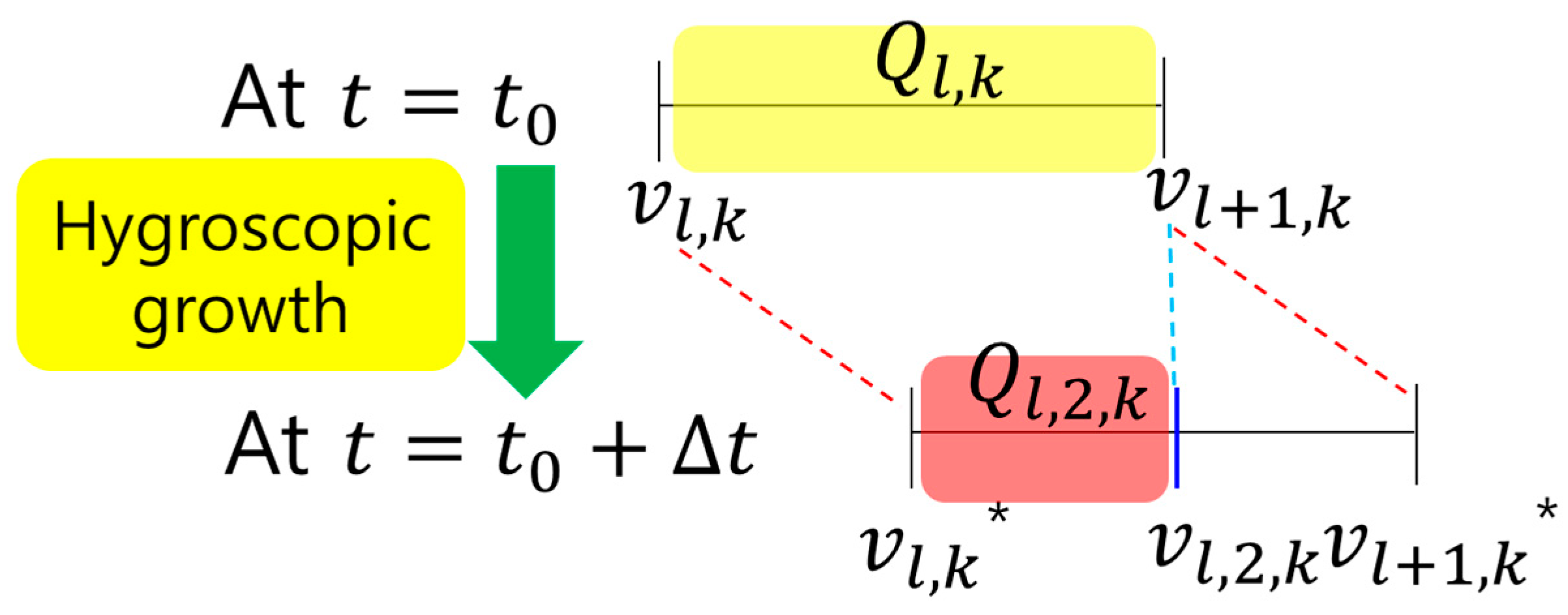
- trl,k: fraction of the aerosol particles of component k in section l that grow up to section l + 1 after hygroscopic growth, which is expressed asThe relationship among the variables delineated in Equations (19)–(24) is shown in Figure 1.
 Figure 1. Concept of change of mass concentration due to hygroscopic growth.
With the results of frl,k and trl,k, an elemental transition matrix that satisfies the following can be constructed:
where
λl,k: transition rate of aerosol particles of component k in section l, defined as
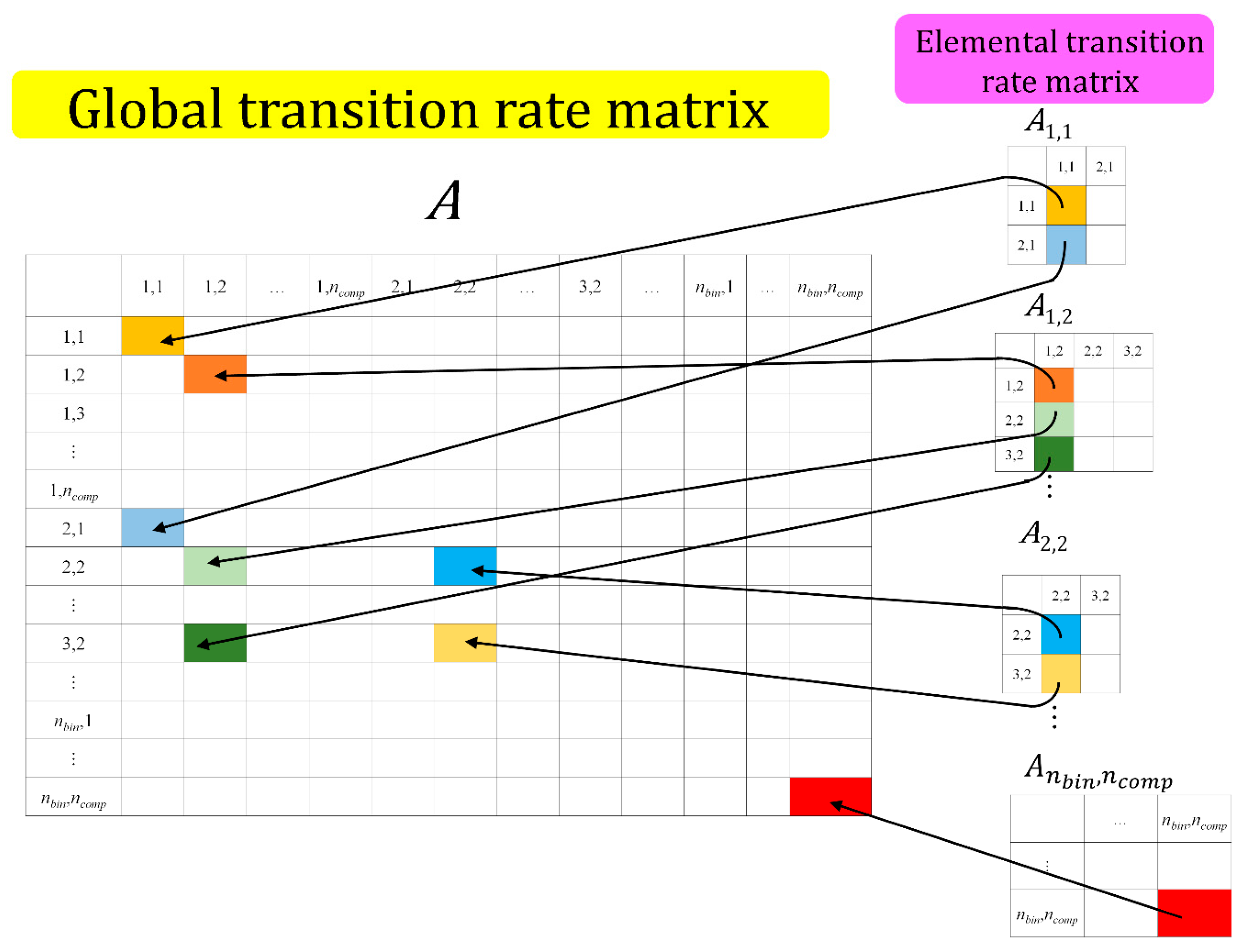
A global transition rate matrix of hygroscopic growth is obtained with elemental transition rate matrices for all components and sections in the analysis as the follows:
where
- nbin: number of sections of the aerosol particles considered in the multicomponent sectional equations.
The process of obtaining the global transition rate matrix can be expressed as illustrated in Figure 2.

Figure 2.
Construction of a global transition rate matrix of hygroscopic growth [19].
In I-COSTA, the following non-homogeneous system of equations is implemented as a way of coupling the multicomponent sectional equations and Mason equations rigorously via the global transition rate matrix:
where
- : mass concentration of aerosol particles of component k that remain in section l after hygroscopic growth for the time step of Δt.
2.3. Comparison of the Coupling Scheme in I-COSTA and That in the Conventional Codes
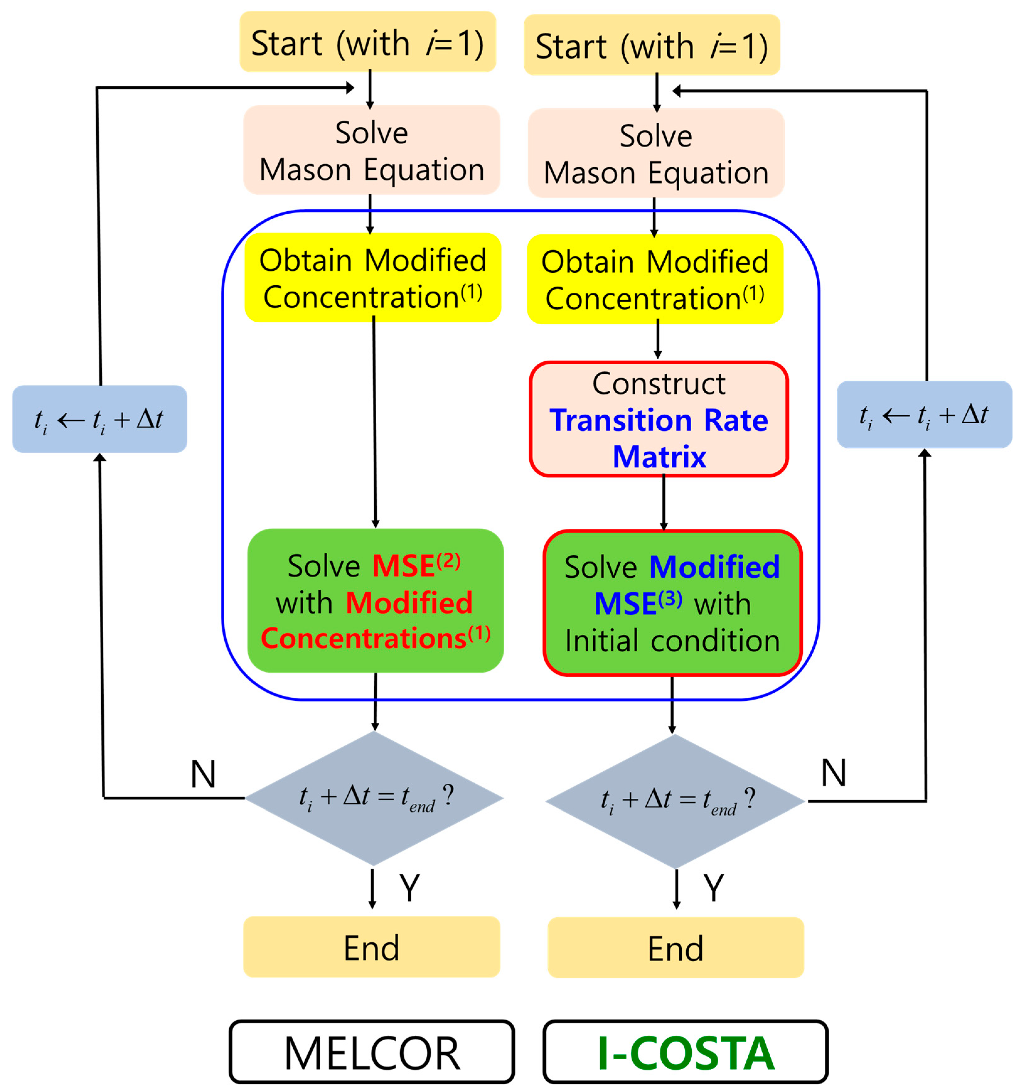
In order to compare the coupling scheme in the I-COSTA and that in conventional code, e.g., MELCOR, comparative calculations are performed on the aerosol behaviors with the hygroscopic growth. In I-COSTA, the coupling scheme is applied to the calculation as discussed in Section 2.2. In the MELCOR code, Mason equations are solved first and then the solutions are used for the initial condition of multicomponent sectional equations for the current time step, since it is assumed that the time scale in hygroscopic growth is much shorter than that of phenomena dealt with in the multicomponent sectional equations in MELCOR [23]. The difference between the two schemes is shown in Figure 3. It should be noted that the main difference is in the use of the transition matrix.

Figure 3.
Comparison of the coupling scheme in MELCOR and I-COSTA used in the aerosol dynamics. (1) Refer to Equations (21) and (22). (2) Refer to Equation (1). (3) Refer to Equation (29).
The changes in airborne concentration using a scenario were compared. This scenario involved aerosol particles with intermediate solubility, i.e., with a Van’t Hoff factor of approximately 1. Geometric and thermophysical conditions of the problem are shown in Table 1. In the problem, behaviors of the aerosols are analyzed for 200 s.

Table 1.
Geometric and thermophysical conditions for the test problems.
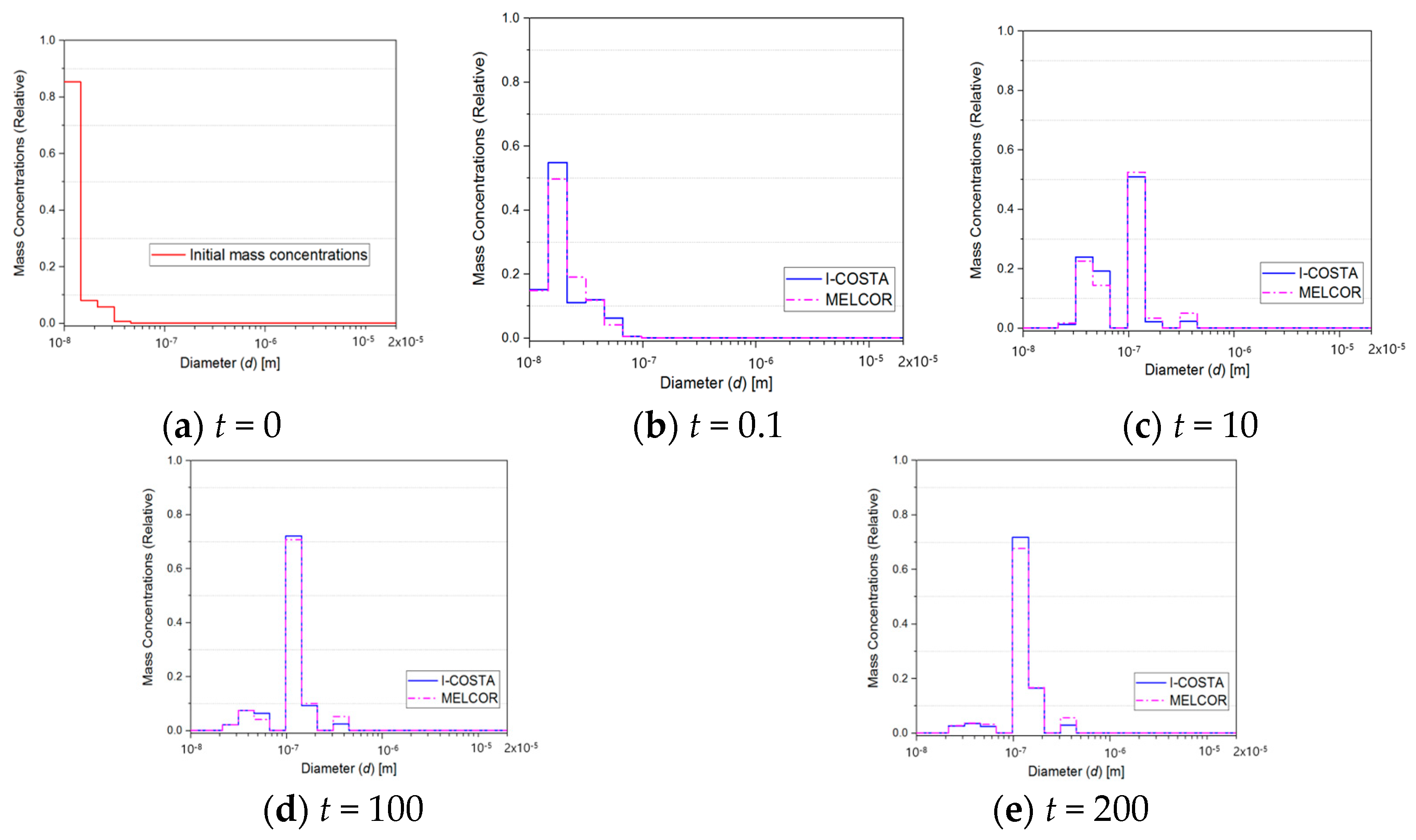
The saturation ratio and the effective saturation ratio on the aerosol particles are assumed to be 1.00005 and 1. Temperature-dependent chemical and thermophysical properties used in the calculations are taken from MELCOR 2.2 [23]. The two codes use 1.0 × 10⁻² s as a size of the time step (Δt). Distribution of mass concentrations of the aerosols at the initial condition is shown in Figure 4. Distributions of mass concentrations at t = 0.1, 10, 100, and 200 s are also shown in Figure 4.
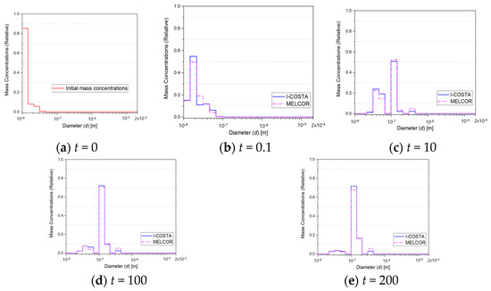
Figure 4.
Distribution of mass concentrations for the test problem; (a) at t = 0; (b) at t = 0.1; (c) at t = 10; (d) at t = 100; (e) at t = 200.
As shown in Figure 4, aerosol particles grow more slowly in I-COSTA than in MELCOR. For example, at t = 200 s, relative mass concentration in sections higher than 10 (d ≥ ) is 0.23 in MELCOR, whereas it is 0.19 in I-COSTA. The reason for this difference is that, as Figure 3 shows, MELCOR uses the solutions of the Mason equations at each time step as the initial conditions for the multicomponent sectional equations. This approach is unrealistic because aerosol particles grow through simultaneous processes of hygroscopic growth and coagulation. In contrast, I-COSTA explicitly couples the two equations and solves them simultaneously. Such differences in numerical methods can lead to variations in the predicted airborne concentrations of aerosol particles in the containment atmosphere during a severe accident—particularly for cesium-related aerosols (e.g., CsOH, CsI, and others), whose behavior strongly depends on hygroscopic growth due to their high solubility in water. It is important to note that cesium is one of the most significant nuclides, as it has a relatively long half-life and a high dose conversion factor, both of which contribute to a high exposure dose rate in the event of a large release caused by containment failure during a severe accident.
The aforementioned differences in the coupling scheme result in variations in the airborne concentrations of aerosols, as demonstrated in the KAEVER experiments referenced in the work by one of the authors [21]. In that study, I-COSTA produced more conservative results than other conventional codes when aerosol particles exhibited low solubility. However, when the particles had high solubility, the coupling scheme yielded results similar to those of the other codes. Currently, information on the solubility of iodine-related aerosol particles is not available, and thus, the coupling scheme used in I-COSTA should be taken into consideration.
2.4. Selected Parameters and Their Uncertainty Range for Importance Analysis
As discussed in the previous section, I-COSTA considers multicomponent sectional equations and Mason equations. For the derivation of the two aforementioned equations from the motion of particles in the gaseous media, numerous phenomenological parameters are used to describe characteristics of the aerosols, such as correction for the deviation from a perfect spherical shape of the particles, non-continuum regime, etc. A database for those parameters is obtained through experiments and/or theoretical derivation, and the parameters are known to have uncertain values, which induces phenomenological uncertainty in the aerosol dynamics [17,18]. In this paper, the authors have considered 12 parameters for the importance analysis. The 12 parameters are incorporated into the coagulation and deposition kernels, as shown in Equations (2)–(12), and are essential for determining the airborne concentrations of aerosol particles in the containment area. It is important to note that the accident source term for radiological consequence analysis is directly determined by the aerosol concentration at the time of containment failure. The characteristics of each parameter are discussed below:
(1) Sticking efficiency () is considered in the coagulation of two particles, as shown in Equations (4), (6) and (A2) in Appendix A. It considers the effect via Van der Walls forces, changes in surface free-energies, and/or chemical reaction [16]. The computer codes on the aerosol dynamics, e.g., MAEROS [21,24], MELCOR [23], etc., have used unity as the value sticking efficiency. According to a previous study [17], the sticking efficiency has an uncertainty range of 0.1 to 1.
(2) Slip correction factor () in Equation (A1), used in Equation (8), arises in the various expressions on the coagulation kernels; it accounts for deviation from continuum mechanics and is derived from the experimental data on spherical parameters. Most of the computer codes for the aerosol dynamics have used 1.37 as a default value. The uncertainty range of the slip correction factor is from 1.1 to 1.4, according to previous studies [17,18,19].
(3) Diffusion boundary thickness () is considered in the Brownian diffusion used for the deposition kernel, as shown in Equation (12). According to the computer codes for aerosol dynamics, such as MAEROS [25], MELCOR [24], etc., the default value of 1.0 × 10⁻⁵ m is widely used, and its uncertainty range is from 10−6 to 10−4 m [14,15,16].
When two particles coagulate, the resulting combined particle does not form a perfect sphere, which affects the behavior of aerosols during a severe accident. In addition, most of the equations for aerosol coagulation are derived theoretically, assuming that the resulting particles are perfectly dense spherical particles. However, in reality, the particles do not have the aforementioned geometry. Therefore, in the aerosol dynamics, two correction factors are introduced to consider the deviation between theoretical derivations and the actual particle characteristics: (4) a dynamic shape factor () and (5) a collision shape factor (), as shown in Equations (5)–(8), (11), etc. The dynamic shape factor describes the difference in the drag force between a perfectly spherical particle and a non-spherical, porous particle. Meanwhile, the collision shape factor accounts for the difference in terms of spatial extent between a perfectly spherical particle and a non-spherical, porous particle. In the current aerosol dynamics codes, the values of the two shape factors are assumed to be unity. In this work, based on the literature, the authors assumed that the two parameters have an uncertainty range from 1 to 4 in the case of severe accident conditions [17,18,19].
(6) The thermal accommodation coefficient (αT) used in Equations (10) and (18) accounts for the interaction between gas and aerosol particles in terms of temperature, and it is known to be strongly dependent on the structure of gas molecules [17,18,19]. The conventional codes have used unity as the value of the coefficient. From a previous study [18], the authors assume an uncertainty range from 0.5 to 1.5 for the importance analysis.
During the motion of particles along the streamline of the fluid, turbulent coagulation may occur as particles collide with each other due to differences in inertia, impaction by structure change in the medium, etc. In turbulent coagulation, the turbulent motion of the fluid is one of the key factors in analyzing the phenomenon. (7) The turbulent energy dissipation rate () is considered in the turbulent inertial and shear coagulations, as shown in Equations (7) and (8). It is the rate at which turbulent kinetic energy is converted into thermal energy affecting turbulent motion. In the conventional computer codes, a default value of 10−3 m2/sec3 is used. In the importance analysis, based on the literature review, a range of 5 × 10⁻⁴–1.5 × 10⁻³ is considered [17,18,19].
For the hygroscopic growth of the aerosol particles, the condensation of the vapor to the surface of the aerosol particles is affected by (8) the saturation ratio (S), (9) the effective diffusion coefficient of vapor (), and (10) the effective thermal conductivity of the atmosphere in the containment (), as shown in Equation (14). According to the experimental activities on the aerosol particles [26], the three parameters have an uncertainty range of 7% during the experiment. The authors have considered the aforementioned range for the importance analysis with the input data for ISP No44 [20].
The aerosol particles in the containment area during a severe accident are not composed of a single substance. They are a mixture of the vapor and various kinds of fission products. Therefore, the (11) density of aerosol particles () has uncertainty. In the conventional computer codes [24,25], a value of 1000 kg/m3 is used as a default value, and it is known to be underestimated [17,18] since the value considers the aerosol particles to be wet particles. In the importance analysis, an uncertainty range of 1000–5000 kg/m3 is considered, based on the literature review [17,18].
For the deposition of the aerosol particles, thermophoresis, which is induced by a thermal gradient in the particle, is considered an important mechanism. In the deposition kernel, (12) the ratio of thermal conductivity of the atmosphere to that of particles () is used to consider the aforementioned effect, as shown in Equation (10). The conventional computer codes [24,25] have used a value of 0.05 as a default value, and an uncertainty range of 2 × 10⁻⁴~5 × 10⁻³ is considered in the importance analysis, based on the literature review [17,18]. The aforementioned phenomenological parameters are summarized in Table 2.
Table 2.
Phenomenological parameters in the analysis.
2.5. Summaries of the Framework for Importance Analysis
With the parameters discussed in the previous section, the authors performed an importance analysis on the aerosol behaviors in the containment area. The first step of the analysis is to sample the values of the parameters randomly within the range of uncertainty discussed in Section 2.3. The sampling is based on Latin hypercube sampling, in which the uncertainty range is divided into n non-overlapping intervals on the basis of equal probability for each parameter. The division is based on the probability density function (PDF) given by users. A cumulative distribution function (CDF) is then calculated for each parameter to sample a single value for each parameter in each interval randomly. With n different values of each parameter generated from previous procedures, n vectors are generated by mixing the order of n values. The mixing is completed by picking up the parameters randomly. Note that the dimension of the aforementioned vector is equal to the total number of parameters considered in the importance analysis. The discussed process is conducted using a stand-alone in-house code named R-SAPhe.
Sensitivity analyses on the change of aerosol concentrations are carried out via I-COSTA with the aforementioned n vectors. The correlation coefficients are then calculated using CC-SAPhe in order to show the relationship between the parameters and the figure-of-merit in the importance analyses. The correlation coefficients lie between −1 and 1; a value of −1 means that a parameter has a perfect negative linear relationship with the figure-of-merit, i.e., the parameter increases, the figure-of-merit decreases. A value of 1 means, in contrast, means that a parameter has perfect a positive linear relationship with the figure-of-merit, i.e., the parameter increases, the figure-of-merit increases. Meanwhile, a value of 0 means there is no linear relationship. According to previous studies, if the absolute value of the correlation coefficient is higher than 0.7, it has strong a linear relationship with the parameters [24]. In this analysis, four types of correlation coefficients are considered: Pearson coefficient, Spearmann coefficient, standardized regression coefficient, and partial correlation coefficient [19,25,26,27]. The procedure for the analyses is summarized in Figure 5.
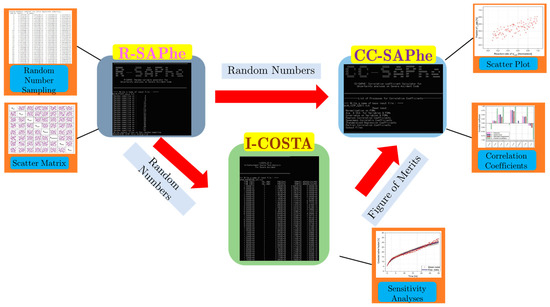
Figure 5.
Importance analysis scheme for the phenomenological parameters with I-COSTA.
3. Numerical Results
3.1. Computation Conditions on the Importance Analysis
In this section, importance analyses are conducted on the phenomenological parameters in I-COSTA. For this analysis, International Standard Problem No. 44 (ISP-44) [20] is considered. ISP-44 consists of five experiments performed using three types of aerosols—CsI, Ag, and CsOH—to examine aerosol behavior with varying solubility. The characteristics of these aerosols are presented in Table 3.
Table 3.
Types of aerosol particles considered in KAEVER experiments.
Among the five ISP-44 experiments, three—KAEVER-148, KAEVER-186, and KAEVER-187—are considered in this study. The KAEVER-148 experiment used Ag aerosols, which have the lowest solubility and exhibit the slowest hygroscopic growth. Importance analysis of this experiment highlights the sensitivity of aerosol behavior to parameters used in the general dynamic equations.
The KAEVER-186 experiment involved a combination of Ag and CsOH aerosols, with CsOH showing the highest solubility and thus the fastest hygroscopic growth. Compared to KAEVER-148, an importance analysis of KAEVER-186 better illustrates the influence of parameters related to hygroscopic growth on aerosol behavior.
The KAEVER-187 experiment used a mixture of all three aerosol types. In comparison to the previous two experiments, the importance analysis of KAEVER-187 reflects the behavior of a broader range of aerosols under conditions closely resembling those in a containment during a severe accident.
All experiments were conducted in the KAEVER facility. The geometric conditions of the KAEVER facility are summarized in Table 4.
Table 4.
Geometric conditions of KAEVER experiments.
For the sensitivity analyses on the change of airborne concentrations of the aerosol particles, I-COSTA is used as discussed in the previous section. The implicit Euler method is used as a numerical method for the time discretization. The Newton method is then used for solving the discretized equations obtained via the implicit method. In the analysis, the step doubling method is used to determine the size of the time step automatically.
In the discretized equations, section-averaged coefficients are required for the calculation of the multicomponent sectional equations, and they are obtained via numerical integrations with Gaussian quadrature. The computation conditions are summarized in Table 5.
Table 5.
Computation conditions of I-COSTTA.
For the importance analysis, it is necessary to determine the appropriate number of samples for the Latin hypercube sampling of phenomenological parameters in aerosol dynamics. In this study, sensitivity analyses on the number of samples were conducted by comparing the averages and standard deviations obtained from various sample sizes with those derived from the continuous distributions of the parameters. Based on this comparison, a sample size of 2000 was selected, as both the average and standard deviation from 2000 samples exhibited a relative difference of less than 10−5 compared to those from the continuous distributions, as shown in Table 6.
Table 6.
Sensitivity studies on the average and standard deviation for various number of samplings in Latin hypercube sampling.
3.2. Importance Analyses on the Phenomenological Parameters for the Aerosol Dynamics
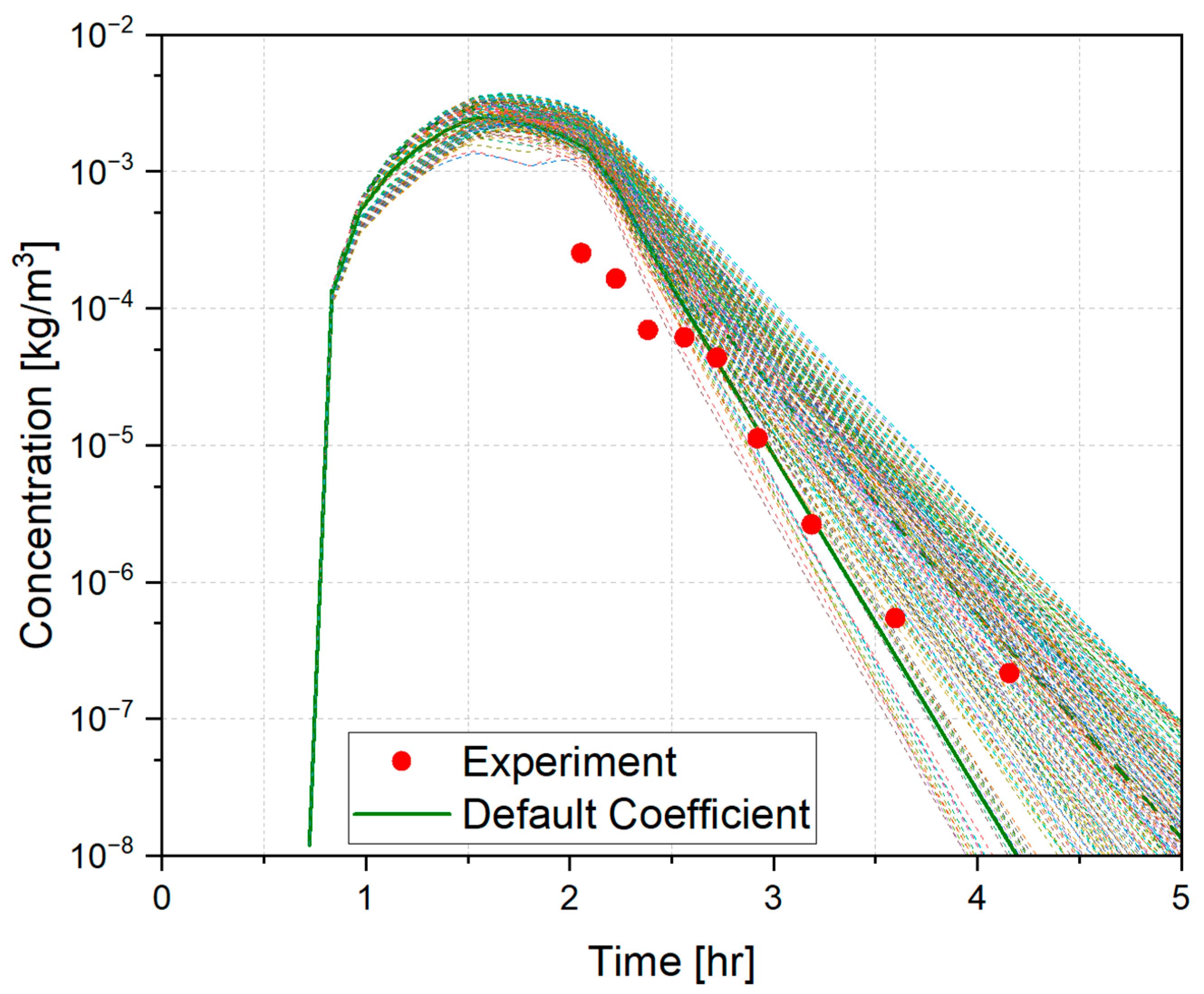
With the aforementioned conditions, the importance analyses are performed on the phenomenological parameters for the aerosol dynamics in I-COSTA. The results of the sensitivity analysis on the KAEVER-148 experiment are shown in Figure 6. The results for the KAEVER-186 and the KAVER-187 experiments are shown in Figure 7 and Figure 8, respectively.
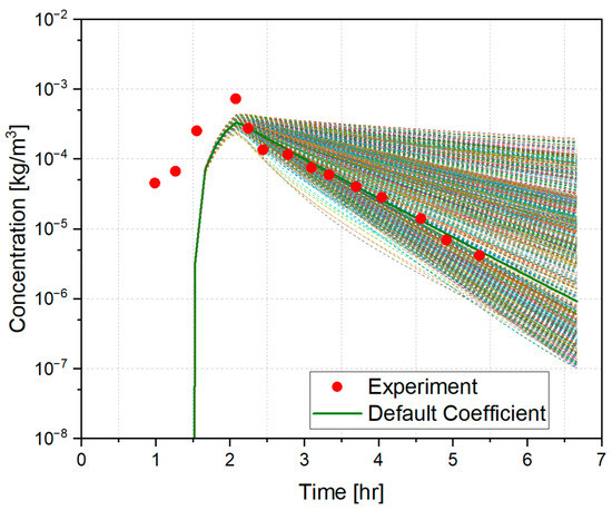
Figure 6.
Sensitivity analysis on the KAEVER-148 experiment with sampling of phenomenological parameters.
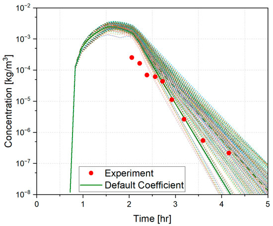
Figure 7.
Sensitivity analysis on the KAEVER-186 experiment with sampling of phenomenological parameters.
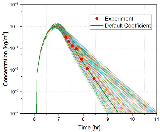
Figure 8.
Sensitivity analysis on the KAEVER-187 experiment with sampling of phenomenological parameters.
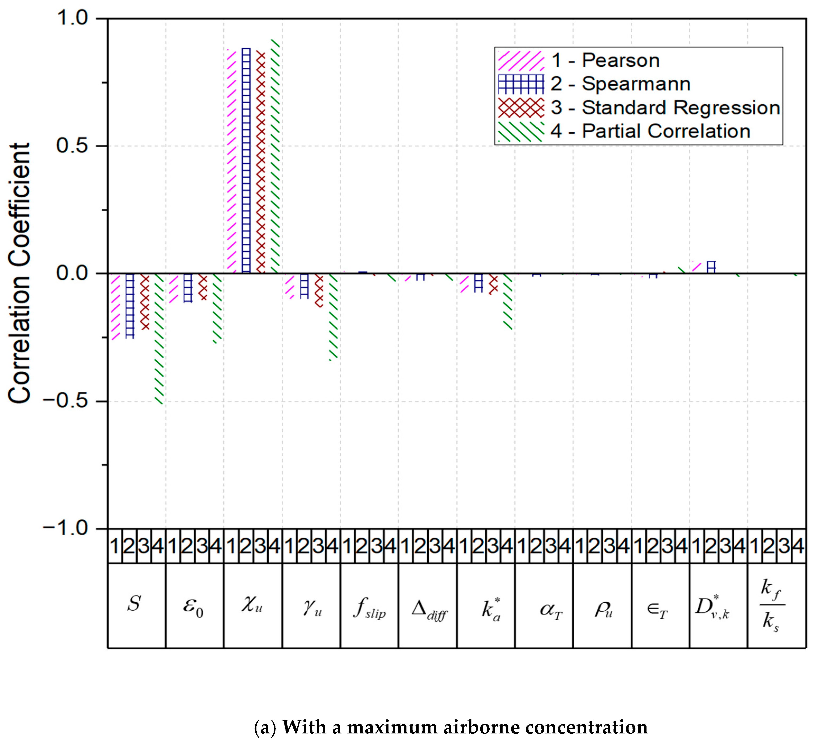
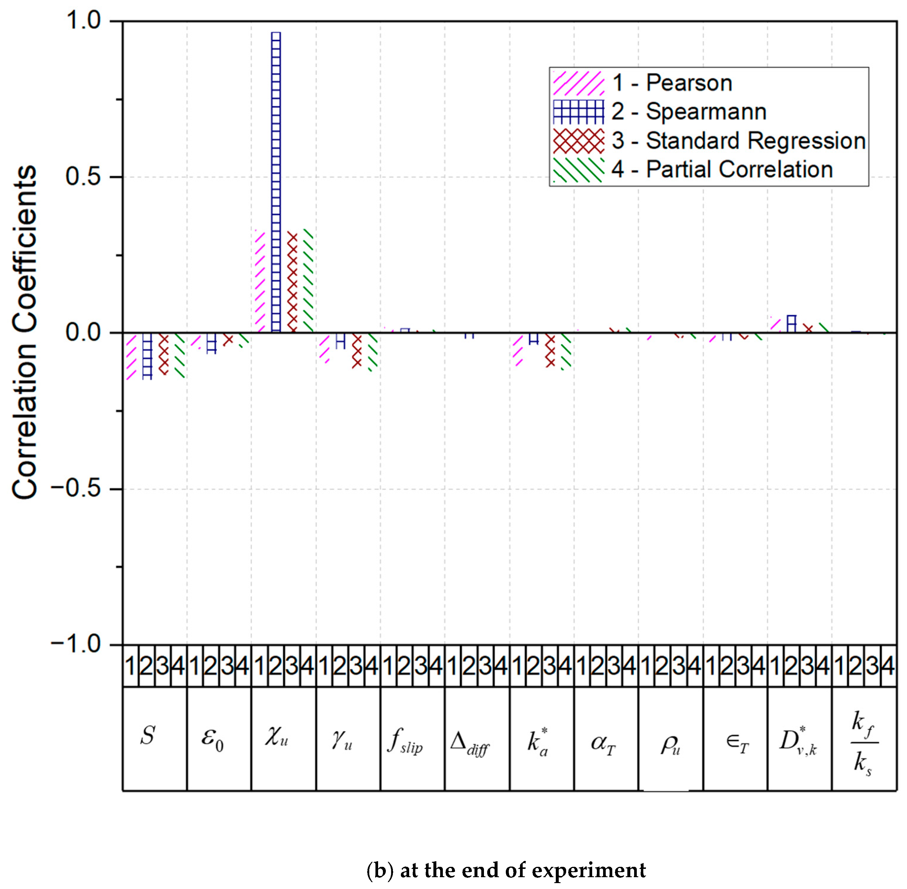
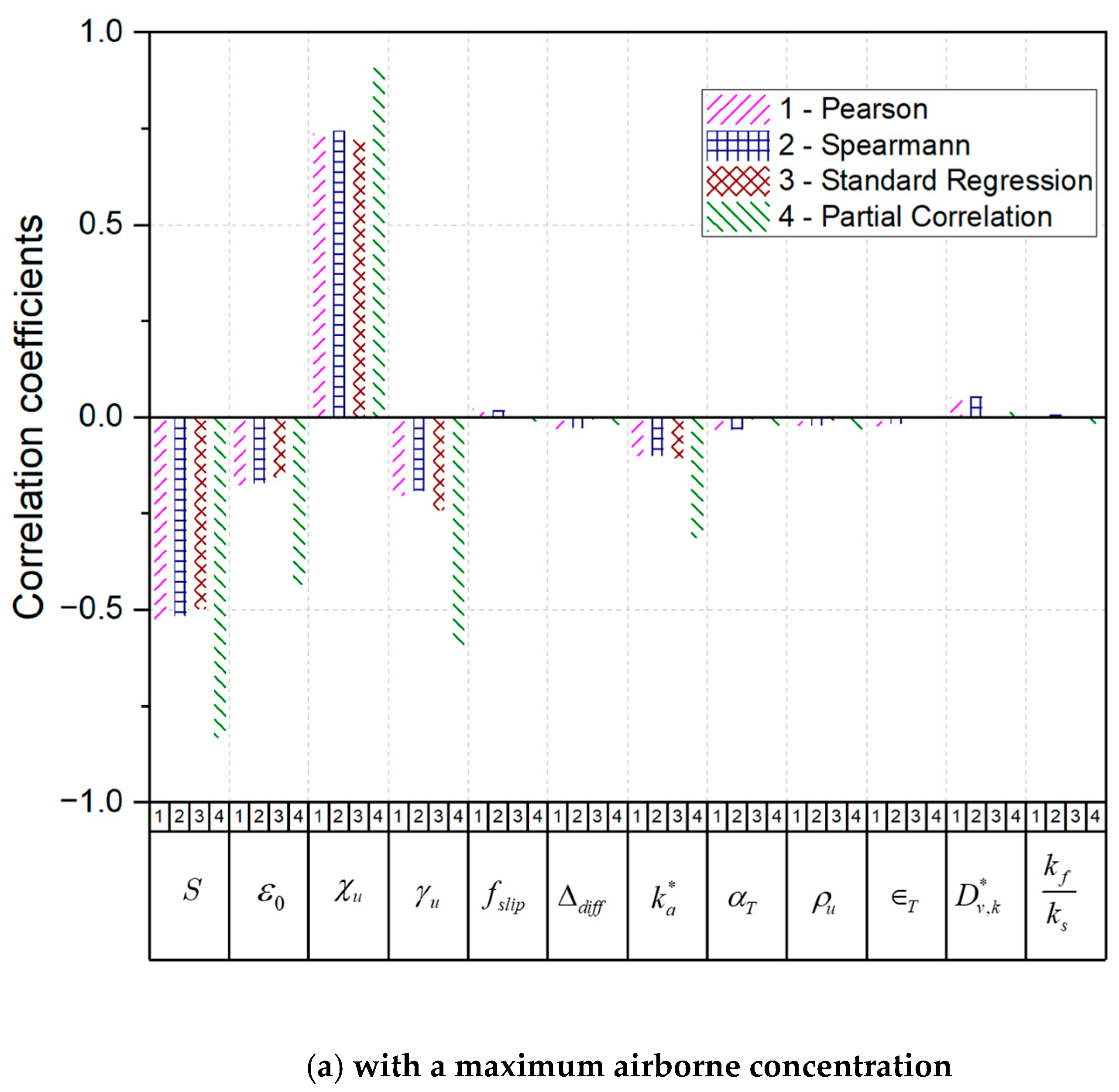
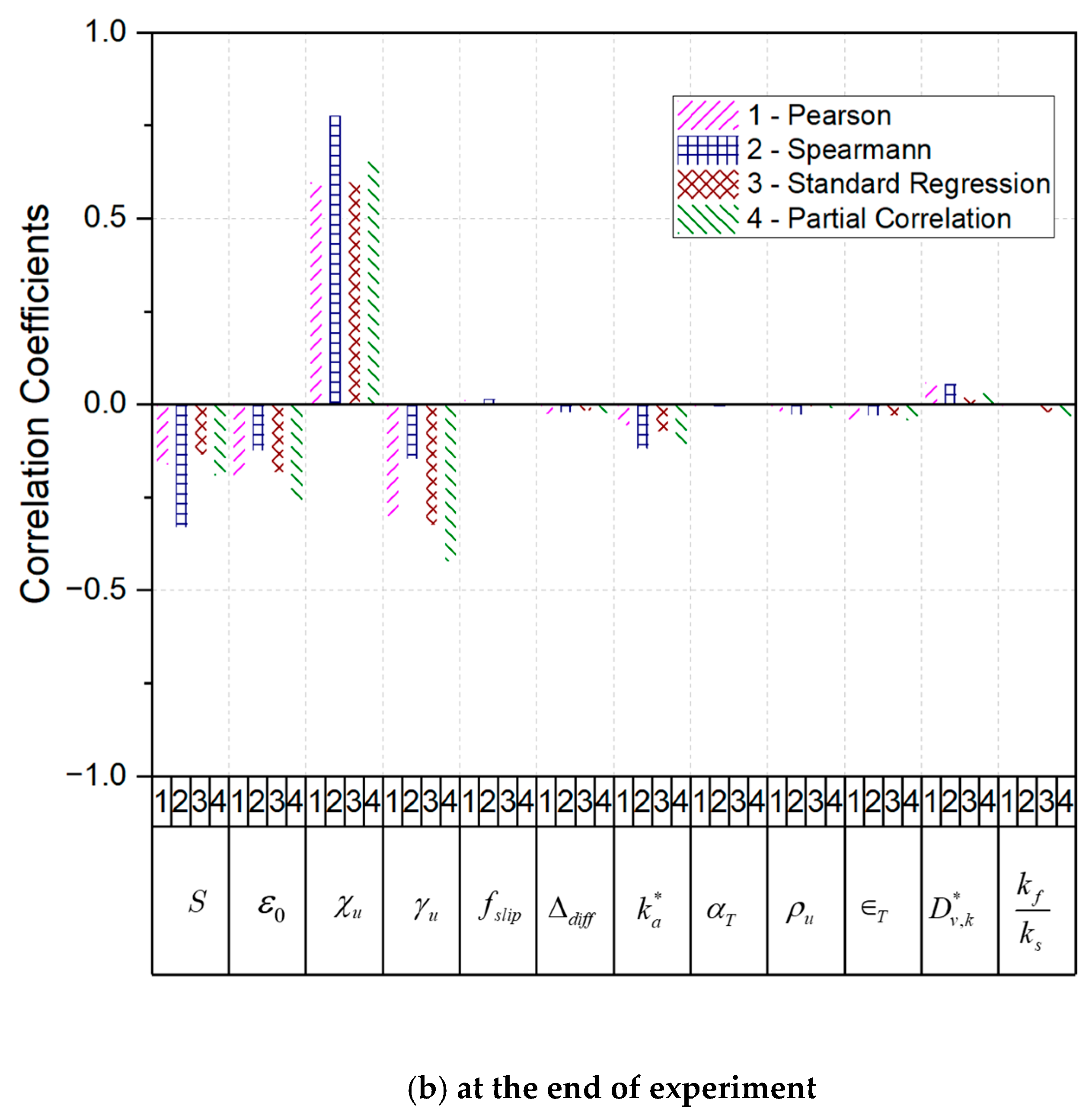
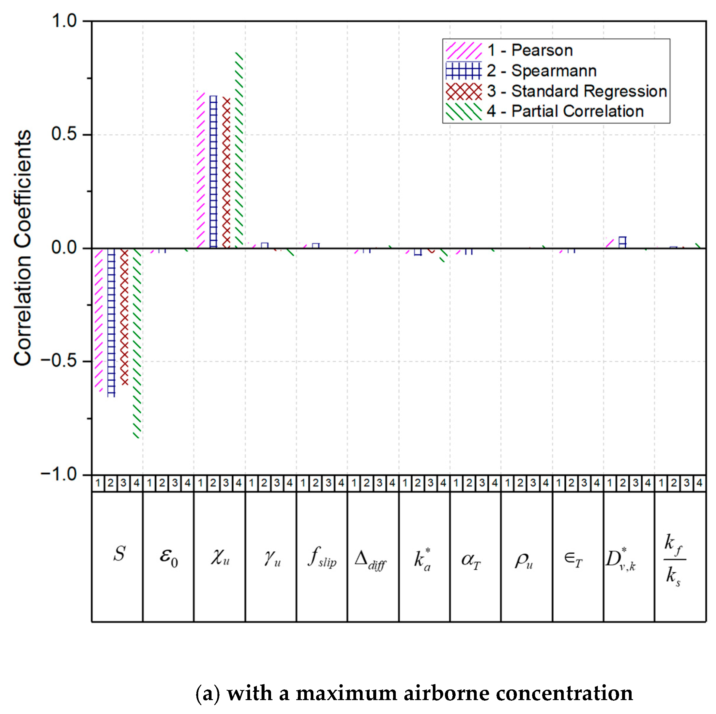
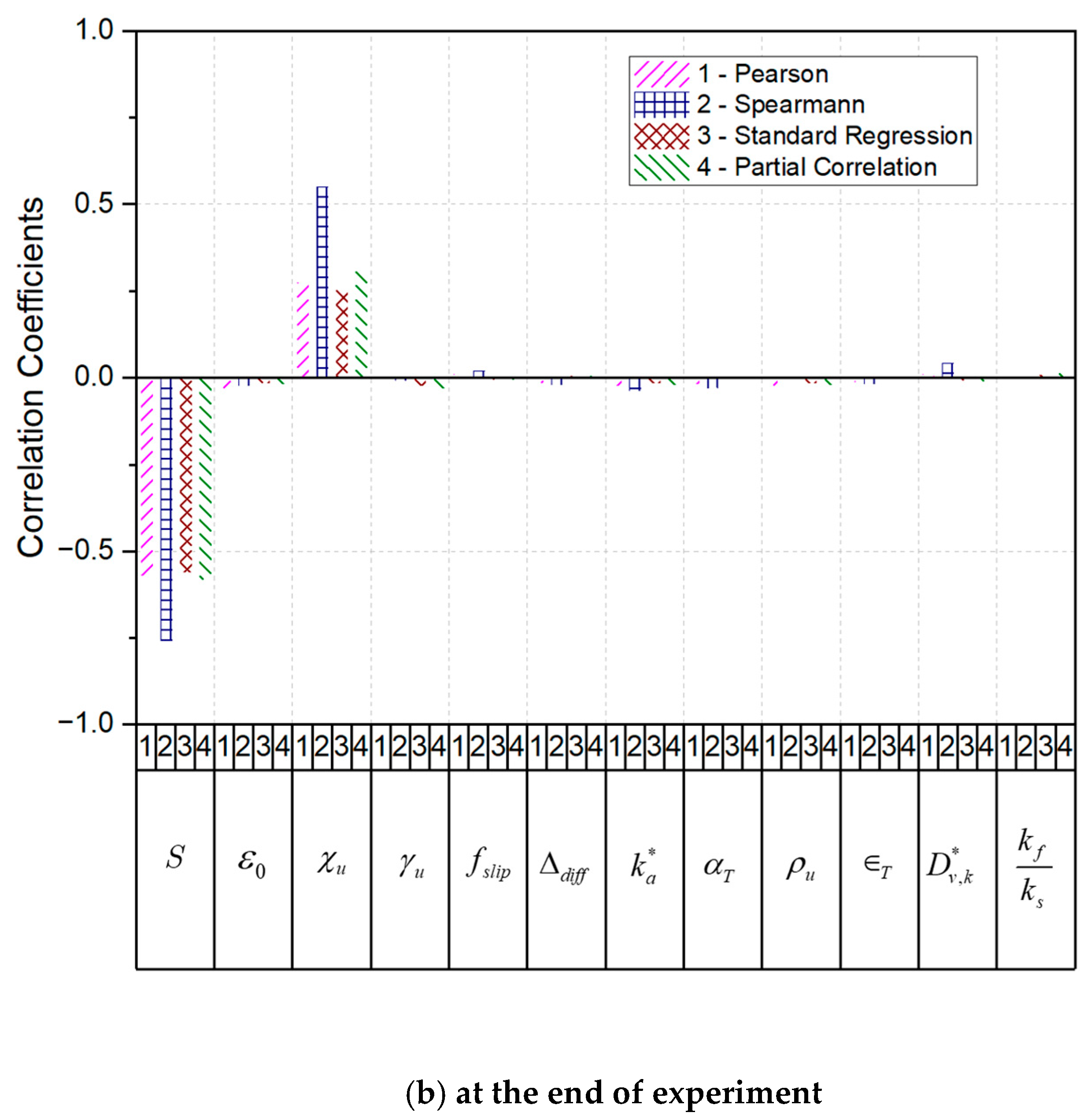
As shown in Figure 6, the change of airborne concentrations of the aerosol particles obtained from the KAEVER-148 experiment is within the range of the sensitivity analysis results via I-COSTA. For the KAEVER-186 and KAEVER-187 experiments, the experimental data on the change of the airborne concentrations are also within the range of the sensitivity analysis results. In terms of the maximum airborne concentrations, the range of sensitivity for the KAEVER-148 experiment is 30% of the values obtained with the reference phenomenological parameters shown in Table 1. Similarly, the range of sensitivity analyses obtained from the other two experiments are 40%, respectively. According to the experimental conditions [20], the range of uncertainty in the measurement of aerosol concentration is known to be 7% of the measured values for most of the experiments in ISP44. This means that the range of sensitivity analyses is much larger than the uncertainty range of the measurement during the experiment. Therefore, we can conclude that the uncertainty in the phenomenological parameters in the aerosol dynamics cause larger uncertainties than those from measurement in terms of the airborne aerosol concentrations. It is thus necessary to analyze the aforementioned parameters in order to enhance the accuracy in the change of aerosol concentrations. Figure 9 shows the correlation coefficients of the phenomenological parameters for the maximum airborne concentrations, and for the airborne concentrations at the end of the experiments obtained from the KAEVER-148 experiment. The correlation coefficients obtained from the other experiments are shown in Figure 10 and Figure 11 for the maximum airborne concentrations and the concentrations at the end of each experiment, respectively.
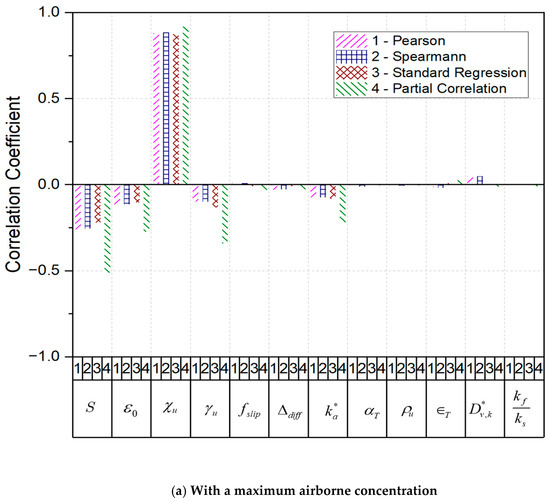
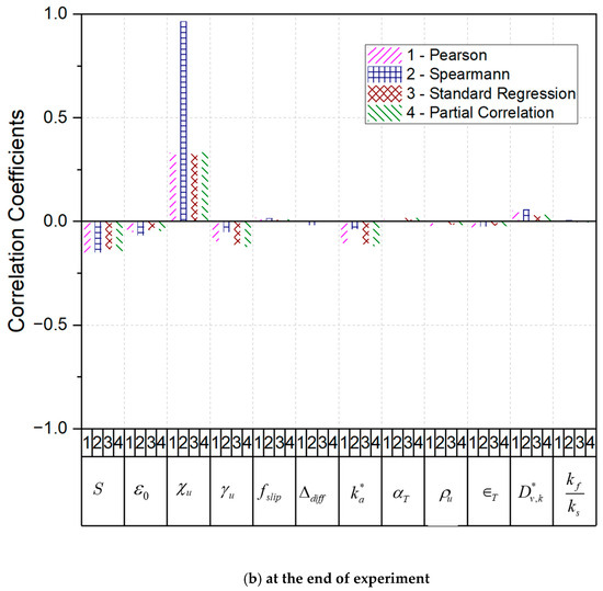
Figure 9.
Correlation coefficients for the KAEVER-148 experiments. (a) With the maximum airborne concentrations, (b) at the end of experiment.
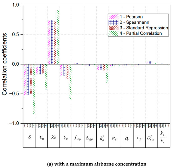
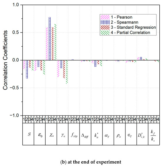
Figure 10.
Correlation coefficients for the KAEVER-186 experiments. (a) With the maximum airborne concentrations, (b) at the end of experiment.
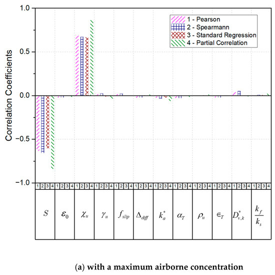
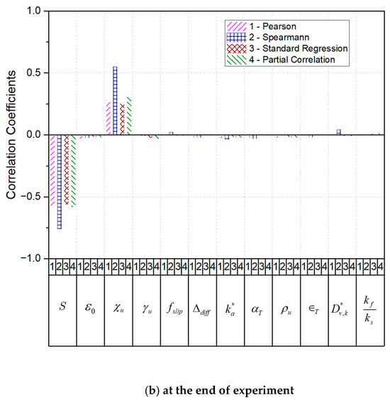
Figure 11.
Correlation coefficients for the KAEVER-187 experiments. (a) With the maximum airborne concentrations, (b) at the end of experiment.
As shown in Figure 9, Figure 10 and Figure 11, the dynamic shape factor shows a strong linear relationship with the airborne concentrations. The airborne concentrations of the aerosol particles decrease as the dynamic shape factor increases. In the aerosol dynamics, the dynamic shape factor is considered in the rate of coagulation of two particles and deposition of the aerosol particles. In the calculation of the coagulation rate, as shown in Equation (4), the dynamic shape factor is used in Brownian, gravitational, and turbulent coagulation kernels, and it is inversely proportional to the rates since the drag force on the non-spherical particle is greater than that on the perfectly spherical particle. In other words, the higher the value of the dynamic shape factor, the smaller the values are in the coagulation kernels. This leads to slower coagulation rates of the aerosol particles, which causes the mass of the aerosol particles in the atmosphere to increase more slowly; this is a key factor in determining the deposition rate.
The dynamic shape factor is also used in the deposition kernels, as shown in Equation (9). As with the coagulation kernels, the dynamic shape factor is inversely proportional to the kernels for the gravitational settling and turbulent deposition, which means that the higher dynamic shape factor, the slower the deposition rate of the aerosol particles. The combined effects of the dynamic shape factor on the coagulation and deposition kernels implies that the dynamic shape factor should have a strong linear relationship with the airborne concentrations of the aerosol particles.
The saturation ratio also shows a strong linear relationship with the airborne concentrations of the aerosol particles. In I-COSTA, the saturation ratio is used in the Mason equations, which determine the hygroscopic rate shown in Equation (13). A higher saturation ratio leads to a faster growth rate of the aerosol particles. A fast growth rate is related to a fast increase of the aerosol particle mass, which leads to a faster particle deposition rate. The saturation ratio, therefore, must show a negative linear relationship with the airborne mass of the aerosol particles.
4. Summary and Conclusions
In this study, importance analyses on the twelve phenomenological parameters for the aerosol dynamics were performed with I-COSTA. The twelve parameters were selected from a review of the literature on the uncertainty of the phenomenological parameters [17,18,19] and uncertainty during measurement [26]. In the importance analyses, the parameters were sampled via Latin hypercube sampling. Sensitivity analyses were then performed on the change of the airborne concentrations of KAEVER-148, KAEVER-186, and KAEVER-187 experiments, which are included in International Standard Problem No. 44 [20]. With the results of the sensitivity analyses, the correlation coefficients between the phenomenological parameters and the maximum airborne concentrations of the aerosol particles were obtained. The correlation coefficients between the aforementioned parameters and the airborne concentrations were also obtained. The main findings from the importance analyses on the phenomenological parameters are as follows:
- The range of the phenomenological parameters taken from previous studies leads to 50% of the airborne concentration of the aerosol particles obtained from experimental values.
- The range of sensitivity of the maximum airborne aerosol concentrations is seven times the uncertainty range of the measurement during experiment, i.e., the uncertainty range of the measurement is known to be 7% of the concentrations [17].
- The larger range of sensitivity compared to the range of measurement appears to be caused by the uncertainty range of the phenomenological parameters. In order to make the accuracy of the aerosol dynamics model comparable to that of the experimental measurement, the uncertainty of the parameters should be reduced.
- From the correlation coefficients between the phenomenological parameters and the airborne concentrations, the dynamic shape factor and the saturation ratio were found to be important parameters with respect to the airborne concentrations of the aerosol particles.
From the aforementioned main findings, the dynamic shape factor should be refined in terms of various severe accident conditions, such as pressure, temperature, dose, etc., to gain a better understanding of the aerosol concentrations. Since the dynamic shape factor is known to depend heavily on the pressure of the gas, which would be linked to the difference in the drag force of non-spherical particles and that of perfectly spherical particles [28,29,30,31,32], it is necessary to construct a database for severe accident conditions so that the uncertainty range of the source term during a severe accident analysis can be reduced.
From the perspective of safety analysis—specifically nuclear safety regulation—the main findings of this study can be used to evaluate uncertainties in the accident source term [33] arising from limited information on the shape as well as the physical and chemical characteristics of aerosol particles released during a severe accident. In the licensing review process for radiological consequences, these uncertainties can help define the uncertainty range of the nuclear accident source term due to aerosol behavior. This, in turn, supports more informed and reasonable regulatory decisions regarding radiological consequences.
Throughout the long history of source term research, the effective dose of Cs type aerosol particles such as CsI and CsOH has been highlighted in terms of the public [17,34], as these particles are long-lived isotopes with high affinity to human organs [34]. As the delayed release of the fission product becomes an important area of research, given the findings from the Fukushima accident [35] and the international cooperative research project [9], it is also necessary to specify the shape and the density of the aerosol particles formed from chemical species, such as iodine oxide in the gaseous phase, etc., especially for coupling the aerosol dynamics code and the iodine chemistry code to evaluate the delayed release of the fission products. Note that, as discussed, the shape and density are known to be the main parameters that determine the dynamic shape factor.
As discussed in Section 1, this aspect may become one of the most critical issues during the licensing review process, as SMR licensees seek to minimize the size of the EPZ to enhance the value of SMRs by enabling construction closer to high population density areas. Minimizing the EPZ requires a best-estimate evaluation of the accident source term, for which detailed analyses of aerosol behavior are essential. In such analyses, it is necessary to develop a database on the characteristics of aerosol particles that could be released from the reactor. The main findings of this study will support the prioritization of parameters needed to construct that database.
Funding
This work was supported by research funds for newly appointed professors of Jeonbuk National University in 2024. This work was also supported by the Nuclear Safety Research Program through the Korea Foundation of Nuclear Safety (KoFONS) and Basis Technology Development on Small Modular Reactor Safety Regulation through Regulatory Research Management Agency for SMRs (RMAS) using financial resources granted by the Nuclear Safety and Security Commission (NSSC) of the Republic of Korea (No. RS-2024-00403364; No. Rs-2024-00509141).
Data Availability Statement
Data can be provided upon request.
Conflicts of Interest
The authors declare no conflicts of interest.
Nomenclature
The following nomenclatures are used in this manuscript:
| A | Global transition rate matrix |
| Al,k | Elemental transition rate matrix for aerosol particles of component k in section l |
| ak | Thermal conduction of the latent heat associated with condensation from particles to the atmosphere |
| Ar,k | Activity of the aerosol particles |
| bk | Diffusion of water vapor from the atmosphere to the particle surface of component k |
| Vapor diffusion coefficient for component k | |
| Effective vapor diffusion coefficient for component k | |
| Slip correction factor | |
| Radius function of the aerosol particles for component k with respect to the mass of particles u | |
| frl,k | Fraction of the aerosol particles of component k in section l that remain in section l after hygroscopic growth |
| Thermal conductivity of atmosphere in the containment | |
| Effective thermal conductivity of atmosphere in the containment | |
| Mw | Molecular weight of the water |
| nbin | Number of sections of the aerosol particles considered in the multicomponent sectional equations |
| ncomp | Number of components of the aerosol particles considered in the multicomponent sectional equations |
| no, ni, | Number of Gaussian quadrature sets |
| Vector form of the multicomponent sectional equations of the aerosol particles | |
| Mass concentration of aerosol particles of component k in section l | |
| Mass concentration of aerosol particles of component k that remain section l after hygroscopic growth for the time step of Δt | |
| Mass concentration of aerosol particles of component k that grow up to section l + 1 after hygroscopic growth for the time step of Δt | |
| R | Gas constant |
| Removal rates of the aerosol particles in section l via deposition, | |
| S | Saturation ratio, in other words, relative humidity in the containment |
| Injection rates of the aerosol particles in section l | |
| Sr,k | Effective saturation ratio at the surface of the aerosol particles |
| slopl,k | Slope of the mass concentration function for component k in section l |
| T∞ | Temperature of the atmosphere in the containment |
| trl,k | Fraction of the aerosol particles of component k in section l that grow up to section l + 1 after hygroscopic growth |
| U(u,t) | Deposition via thermophoresis, |
| VT(u) | Deposition via gravitational settling |
| Diffu(u) | Deposition via diffusiophoresis, |
| Abscissas for Gaussian quadrature | |
| ul | Mass of a single aerosol particle in section l |
| v | Mass of a single particle |
| vl | Mass of a single aerosol particle in section l |
| Weights for Gaussian quadrature | |
| xl | Radius of a single aerosol particle in section l |
| αc | Condensation coefficient |
| αT | Thermal accommodation coefficient |
| (u,v) | Kernel for Brownian, gravitational, and turbulent shear coagulations for particles having masses of u and v |
| (u,v) | Brownian coagulation kernel, |
| (u,v) | Gravitational coagulation kernel |
| (u,v) | Turbulent inertial coagulation kernel |
| (u,v) | Turbulent shear coagulation kernel |
| Coagulation rate of the aerosol particles in sections lower than l forming an aerosol particle in section l | |
| Coagulation rate of the aerosol particles in section l and sections lower than l forming an aerosol particle larger than those in section l | |
| Intra-sectional coagulation rate of the aerosol particles in section l forming an aerosol particle larger than those in section l | |
| Coagulation rate of the aerosol particles in section l forming an aerosol particle larger than those in section l | |
| Diffusion boundary thickness | |
| Collision shape factor of an aerosol particle with mass u | |
| Sticking efficiency of the two aerosol particles | |
| Gas viscosity | |
| Mean free path of an aerosol particle, | |
| λl,k | Transition rate of aerosol particles of component k in section l |
| ρw | Density of the water |
| σ | Surface tension of water |
| Dynamic shape factor of an aerosol particle with mass u | |
| Turbulent energy dissipation rate |
Appendix A. Description on the Coefficients Used in Equations (1)–(29)
The followings are the coefficients used in Equations (1)–(29) of the paper
: radius function of the aerosol particles for component k with respect to the mass of particles expressed as
: weights for Gaussian quadrature, satisfying
: weights for Gaussian quadrature, satisfying
References
- Hart, M.; Herviou, K.; Wu, J.; Taehee, K.; Shapovalov, A.; Thomas, K.; Wallace, D. SMR Regulators’ Forum, Pilot Project Report: Report from Working Group on Emergency Planning Zone; International Atomic Energy Agency (IAEA): Wien, Austria, 2018; Available online: https://www.iaea.org/sites/default/files/18/01/smr-rf-report-appendix-iv-29012018.pdf (accessed on 31 May 2025).
- Haste, T.; Payot, F.; Bottomley, P.D.W. Transport and deposition in the Phébus FP circuit. Ann. Nucl. Energy 2013, 61, 102–121. [Google Scholar] [CrossRef]
- Mascari, F.; Bersano, A.; Massone, M.; Agnello, G.; Coindreau, O.; Beck, S.; Tiborcz, L.; Paci, S.; Angelucci, M.; Herranz, L.E.; et al. Main outcomes of the Phebus FPT1 uncertainty and sensitivity analysis in the EU-MUSA project. Ann. Nucl. Energy 2024, 196, 110205. [Google Scholar] [CrossRef]
- Yu, M. Main outputs from the OECD/NEA ARC-F Project. In Proceedings of the 20th International Topical Meeting on Nuclear Reactor Thermal Hydraulics (NURETH-20), Washington, DC, USA, 20–25 August 2023. [Google Scholar]
- Doi, T.; Masumoto, K.; Toyoda, A.; Tanaka, A.; Shibata, Y.; Hirose, K. Anthropogenic radionuclides in the atmosphere observed at Tsukuba: Characteristics of the radionuclides derived from Fukushima. J. Environ. Radioact. 2013, 122, 55–62. [Google Scholar] [CrossRef] [PubMed]
- Grégoire, A.C.; Le Fessant, E.; Cantrel, L. ESTER Program—State of the Art on Revaporization from RCS Surfaces; IRSN No 2021-00282; IRSN: Fontenay-aux-Roses, France, 2021. [Google Scholar]
- Katata, G.; Chino, M.; Kobayashi, T.; Terada, H.; Ota, M.; Nagai, H.; Kajino, M.; Draxler, R.; Hort, M.C.; Malo, A.; et al. Detailed source term estimation of the atmospheric release for the Fukushima Daiichi Nuclear Power Station accident by coupling simulations of an atmospheric dispersion model with an improved deposition scheme and oceanic dispersion model. Atmos. Chem. Phys. 2015, 15, 1029–1070. [Google Scholar] [CrossRef]
- Terada, H.; Katata, G.; Chino, M.; Nagai, H. Atmospheric discharge and dispersion of radionuclides during the Fukushima Dai-ichi Nuclear Power Plant accident. Part II: Verification of the source term and analysis of regional-scale atmospheric dispersion. J. Environ. Radioact. 2012, 112, 141–154. [Google Scholar] [CrossRef] [PubMed]
- Experiments on Source Term for Delayed Releases (ESTER) Project. 2020. Available online: http://www.oecd-nea.org/jcms/pl_58926/experiments-on-source-term-for-delayed-releases-ester-project (accessed on 31 May 2025).
- Colombani, J.; Pascal, C.; Martinet, L.; Duffieux, C.; Boy, G. AER-11 STEM/EPICUR Test Report; Rapport no PLEIADE PSN-RES/SEREX/2014-00365; Institut de Radioprotection et de Surete Nucleaire: Caradache, France, 2014. [Google Scholar]
- Colombani, J.; Planteur, S. AER-4, AER-5 and AER-6 STEM/EPICUR Test Report Formation and Release of Volatile Iodine Species from CsI Aerosols Under Radiation; Rapport no PLEIADE PSN-RES/SEREX/2013-00616; Institut de Radioprotection et de Surete Nucleaire: Caradache, France, 2013. [Google Scholar]
- Leroy, O. ESTER-EPICUR LOCOV Test Report; Rapport no 2022-00313; Institut de Radioprotection et de Surete Nucleaire: Caradache, France, 2023. [Google Scholar]
- Leroy, O.; Bosland, L. Study of the stability of iodine oxides (IxOy) aerosols in severe accident conditions. Ann. Nucl. Energy 2023, 181, 109526. [Google Scholar] [CrossRef]
- Dickinson, S.; Auvinen, A.; Ammar, Y.; Bosland, L.; Clément, B.; Funke, F.; Glowa, G.; Kärkelä, T.; Powers, D.A.; Tietze, S.; et al. Experimental and modelling studies of iodine oxide formation and aerosol behaviour relevant to nuclear reactor accidents. Ann. Nucl. Energy 2014, 74, 200–207. [Google Scholar] [CrossRef]
- Funke, F.; Langrock, G.; Kanzleiter, T.; Poss, G.; Fischer, K.; Kühnel, A.; Weber, G.; Allelein, H.-J. Iodine oxide in large-scale THAI tests. Nucl. Eng. Des. 2012, 245, 206–222. [Google Scholar] [CrossRef]
- Allelein, H.-J.; Auvinen, A.; Ball, J.; Gűntay, S.; Herranz, L.E.; Hidaka, A.; Jones, A.V.; Kissane, M.; Powers, D.; Weber, G. State-of-the-Art Report on Nuclear Aerosols; NEA/CSNI/R(2009)5; Organisation for Economic Co-operation and Development (OECD) Nuclear Energy Agency (NEA): Boulogne-Billancourt, France, 2009. [Google Scholar]
- Powers, D.A.; Washington, K.E.; Burson, S.B.; Sprung, J.L. A Simplified Model of Aerosol Removal by Natural Processes in Reactor Containments; NUREG/CR-6189; U.S. NRC: Washington, DC, USA, 1996.
- Malicki, M.; Lind, T. Parametric MELCOR 2.2 sensitivity and uncertainty study with a focus on aerosols based on Phebus test FPT1. Prog. Nucl. Energy 2023, 158, 104609. [Google Scholar] [CrossRef]
- Firnhaber, M.; Fischer, K.; Schwarz, S.; Weber, G. International Standard Problem ISP44 KAEVER Experiments on the Behavior of Core-melt Aerosols in a LWR Containment–Comparison Report; NEA/CSNI/R (2003) 5; Nuclear Energy Agency (NEA): Boulogne-Billancourt, France, 2003. [Google Scholar]
- Lee, Y.; Cho, Y.J.; Lim, K. Coupling scheme of multicomponent sectional equations and Mason equations via transition rate matrix of hygroscopic growth applied to international standard problem No. 44. Ann. Nucl. Energy 2019, 127, 437–449. [Google Scholar] [CrossRef]
- Gelbard, F.; Seinfeld, J.H. Simulation of multicomponent aerosol dynamics. J. Colloid Interface Sci. 1980, 78, 485–501. [Google Scholar] [CrossRef]
- Pruppacher, H.R.; Klett, J.D. Microphysics of Clouds and Precipitation; D. Reidel Publishing Co.: Dordrecht, The Netherlands, 1980. [Google Scholar]
- Gauntt, R.O.; Cole, R.K.; Erickson, C.M.; Gido, R.I.; Gasser, R.D.; Rodriguez, S.B.; Young, M.F. MELCOR Computer Code Manuals Vol. 2: Reference Manual, Version 1.8.6; NUREG/CR-6119; Sandia National Laboratories: Albuquerque, NM, USA, 2001. [Google Scholar]
- Gelbard, F. MAEROS User Manual; NUREG/CR-1391, SAND80-0822; Sandia National Laboratories: Albuquerque, NM, USA, 1982. [Google Scholar]
- Rovelli, G.; Miles, R.E.H.; Reid, J.P.; Clegg, S.L. Accurate Measurements of Aerosol Hygroscopic Growth over a Wide Range in Relative Humidity. J. Phys. Chem. A. 2016, 120, 4376–4388. [Google Scholar] [CrossRef] [PubMed]
- Ratner, B. The correlation coefficient: Its values range between +1/−1, or do they? J. Target. Meas. Anal. Market. 2009, 17, 139–142. [Google Scholar] [CrossRef]
- Cohen, J.; Cohen, P.; West, S.G.; Aiken, L.S. Applied Multiple Regression/Correlation Analysis for the Behavioral Sciences, 3rd ed.; Lawrence Erlbaum Associate Inc.: Mahwah, NJ, USA, 2003. [Google Scholar]
- Iman, R.L.; Shortencarier, M.J. A FORTRAN 77 Program and User’s Guide for the Generation of Latin Hypercube and Random Samples for Use with Computer Models; NUREC/CR-3624, SAND83-2365; Sandia National Laboratories: Albuquerque, NM, USA, 1984. [Google Scholar]
- Lee, Y.; Cho, Y.J. Preliminary importance analyses on model for pH in the presence of organic impurities in the aqueous phase for a severe accident of a nuclear power plant. Nucl. Eng. Technol. 2024, 56, 2079–2091. [Google Scholar] [CrossRef]
- Hansson, H.C.; Ahlberg, M.S. Dynamic shape factors of sphere aggregates in an electric-field and their dependence on the Knudsen number. J. Aero. Sci. 1985, 16, 69–79. [Google Scholar] [CrossRef]
- Hochrainer, D.; Hänel, G. Der dynamische formfaktor nicht-kugelf¨ormiger teilchen als funktion des luftdrucks. J. Aero. Sci. 1975, 6, 97–103. [Google Scholar] [CrossRef]
- Wang, S.; Zhou, K.; Lu, X.; Chen, H.; Yang, F.; Li, Q.; Chen, J.; Prather, K.A.; Yang, X.; Wang, X. Online shape and density measurement of single aerosol particles. J. Aero. Sci. 2022, 159, 105880. [Google Scholar] [CrossRef]
- Soffer, L.; Burson, S.B.; Ferrell, C.M.; Lee, R.Y.; Ridgely, J.N. Accident Source Terms for Light-Water Nuclear Power Plants; NUREG-1465; U.S. NRC: Washington, DC, USA, 1995.
- ICRP. Annuals of the ICRP. ICRP Publication 119. Compendium of Dose Coefficients Based on ICRP Publication 60; Elsevier: Amsterdam, The Netherlands, 2012; Volume 41 (Suppl. 1). [Google Scholar]
- Fukushima Daiichi Nuclear Power Station Accident Information Collection and Evaluation (FACE) Project. 2022. Available online: https://www.oecd-nea.org/jcms/pl_70741/fukushima-daiichi-nuclear-power-station-accident-information-collection-and-evaluation-face-project (accessed on 31 May 2025).


Disclaimer/Publisher’s Note: The statements, opinions and data contained in all publications are solely those of the individual author(s) and contributor(s) and not of MDPI and/or the editor(s). MDPI and/or the editor(s) disclaim responsibility for any injury to people or property resulting from any ideas, methods, instructions or products referred to in the content. |
© 2025 by the author. Licensee MDPI, Basel, Switzerland. This article is an open access article distributed under the terms and conditions of the Creative Commons Attribution (CC BY) license (https://creativecommons.org/licenses/by/4.0/).