Real-Time Classification of Distributed Fiber Optic Monitoring Signals Using a 1D-CNN-SVM Framework for Pipeline Safety

Abstract

The growing reliance on natural gas in urban China has heightened the urgency of maintaining pipeline integrity, particularly in environments prone to disruption by nearby construction activities. In this study, we present a practical approach for the real-time classification of distributed fiber optic monitoring signals, leveraging a hybrid framework that combines the feature learning capacity of a one-dimensional convolutional neural network (1D-CNN) with the classification robustness of a support vector machine (SVM). The proposed method effectively distinguishes various pipeline-related events—such as minor leakage, theft attempts, and human movement—by automatically extracting their vibration patterns. Notably, it addresses the common shortcomings of softmax-based classifiers in small-sample scenarios. When tested on a real-world dataset collected via the DAS3000 system from Hangzhou Optosensing Co., Ltd., the model achieved a high classification accuracy of 99.92% across six event types, with an average inference latency of just 0.819 milliseconds per signal. These results demonstrate its strong potential for rapid anomaly detection in pipeline systems. Beyond technical performance, the method offers three practical benefits: it integrates well with current monitoring infrastructures, significantly reduces manual inspection workloads, and provides early warnings for potential pipeline threats. Overall, this work lays the groundwork for a scalable, machine learning-enhanced solution aimed at ensuring the operational safety of critical energy assets.

1. Introduction

1.1. Background

As an essential component of clean energy, natural gas is increasingly prominent in the energy consumption structure, and it is mainly transported by pipeline. However, pipeline transport faces complex safety challenges, especially the potential threats to safe operation related to third-party construction activities. These threats include construction activities such as the use of excavators and ground engineering. If not properly managed, they could cause accidental damage to pipelines, leading to natural gas leaks and posing a risk to public safety. Therefore, developing efficient and accurate natural gas pipeline monitoring technologies is crucial for ensuring the reliability of national energy supply and the stability of economic development [1].

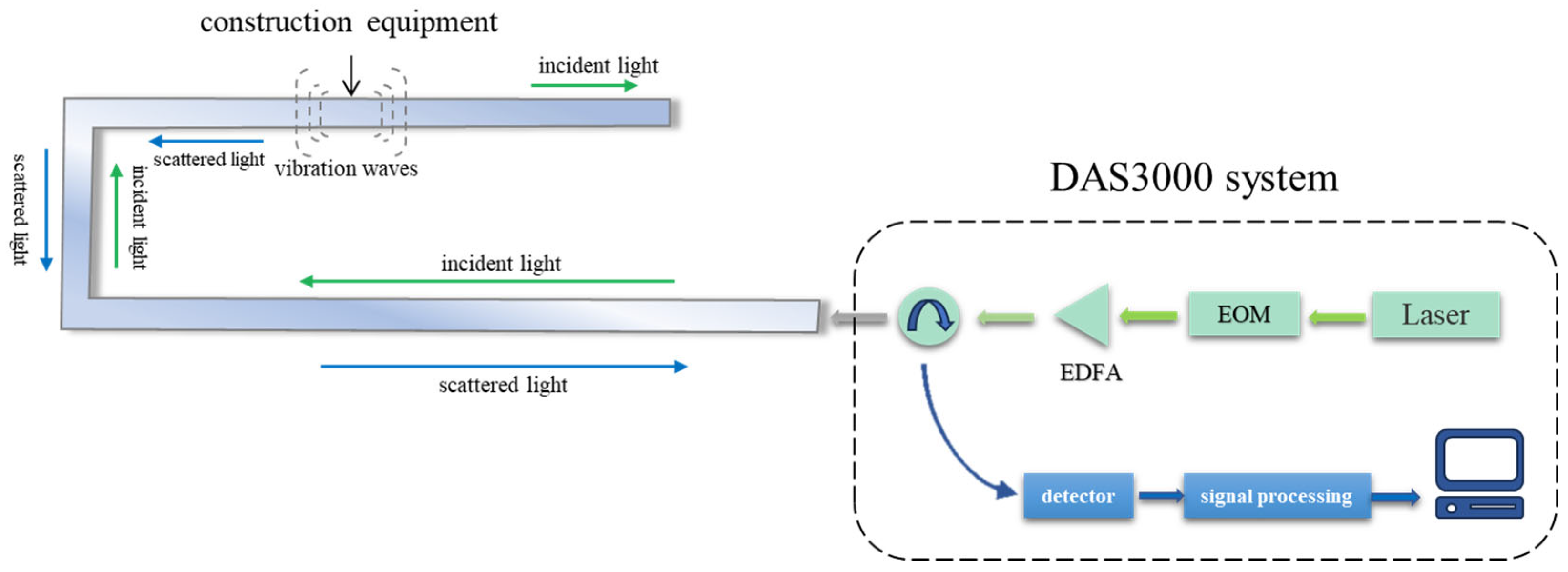
With the continuous advancement of sensing technology, distributed fiber optic monitoring technology has gradually become one of the important means of pipeline monitoring. This technology uses fiber optic sensors laid along the pipeline to leverage the high sensitivity of optical fibers to environmental changes, capturing physical phenomena such as vibrations and temperature changes around the pipeline in real-time, thereby identifying potential threats. 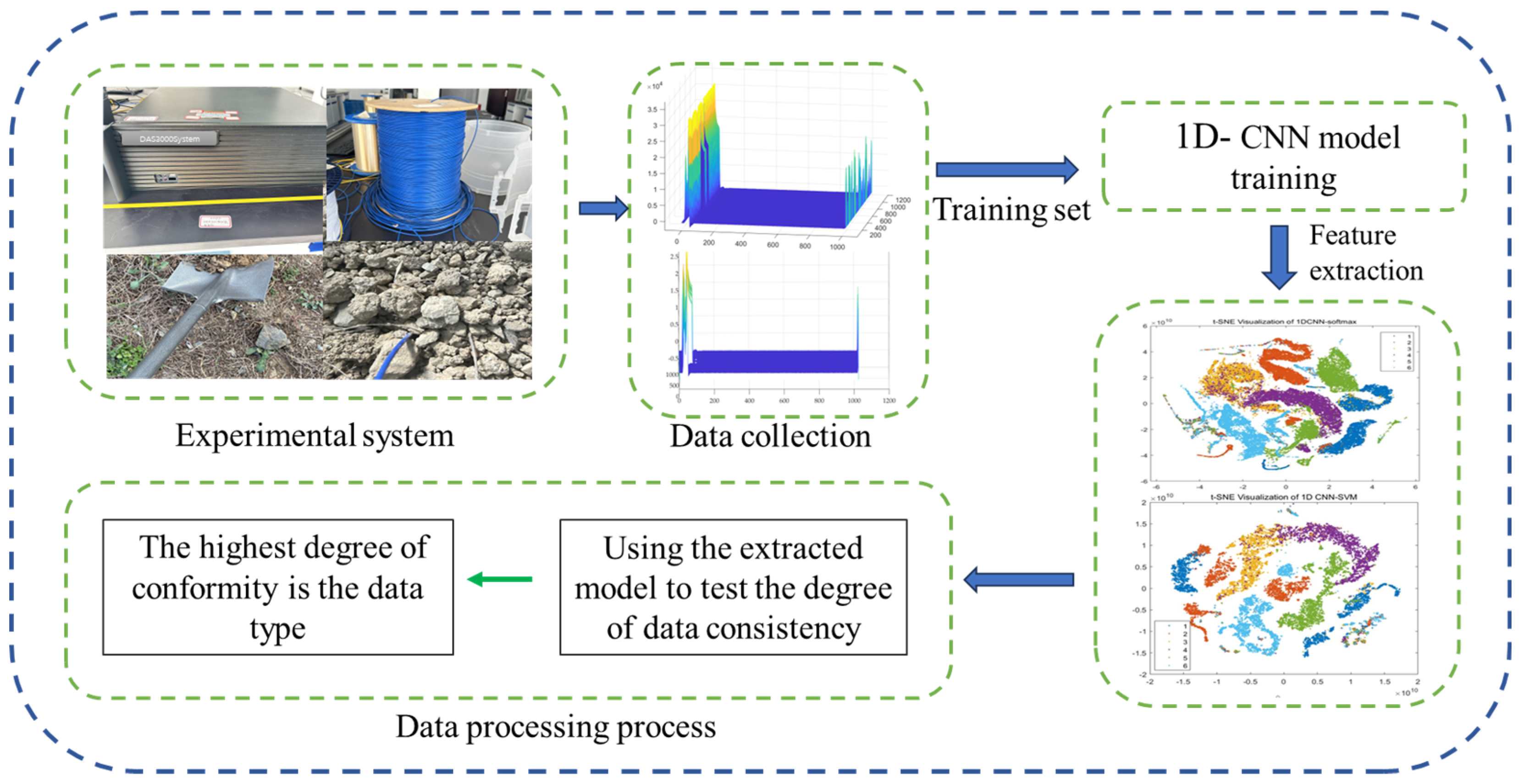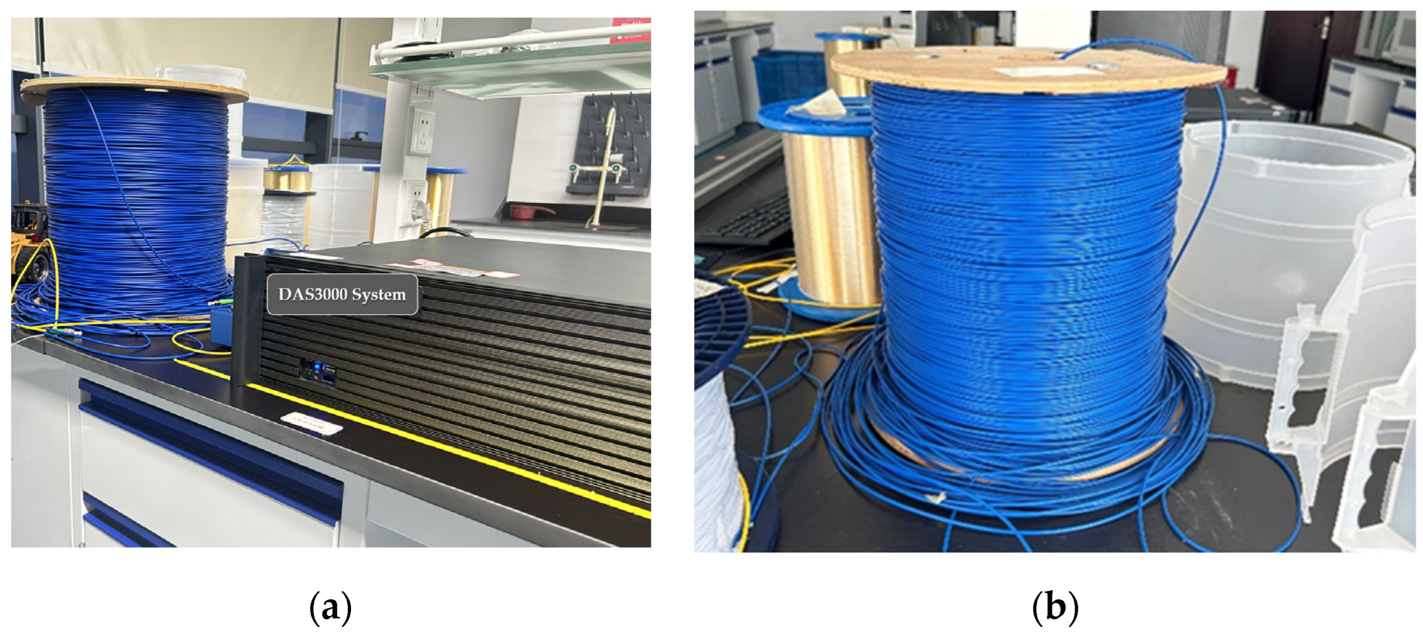However, despite the powerful detection capabilities of fiber optic monitoring systems, extracting useful information from large amounts of noisy raw signals remains a technical challenge that urgently needs to be addressed in practical applications [2]. This paper’s research centers on the safety monitoring of natural gas pipelines in densely populated regions under the impact of third-party construction. Based on the 1D-CNN-SVM algorithm, it extracts useful features from the redundant original signals and classifies the distributed optical fiber monitoring signals in accordance with the features to tackle the challenges in this context. In this context, the integration of advanced machine learning models such as 1D-CNN and SVM with distributed fiber optic sensing systems offers a promising solution. These algorithms enable efficient feature extraction and precise classification of vibration signals associated with different types of pipeline threats. By automating the recognition of abnormal patterns from complex sensor data, the system can provide early warnings for construction activities or accidental impacts, significantly improving the safety and operational management of natural gas pipelines in high-risk urban areas.

1.2. Related Works

Conventional monitoring signal recognition methods require preprocessing of raw signals to extract fault features, such as wavelet transform (WT), ensemble empirical mode decomposition (EEMD) [3], and variational mode decomposition (VMD) [4]. Subsequently, classification algorithms are used to detect fault types, with representative classifiers including back propagation neural networks (BPNN), convolutional neural networks (CNNs), and support vector machines (SVMs) [5,6].

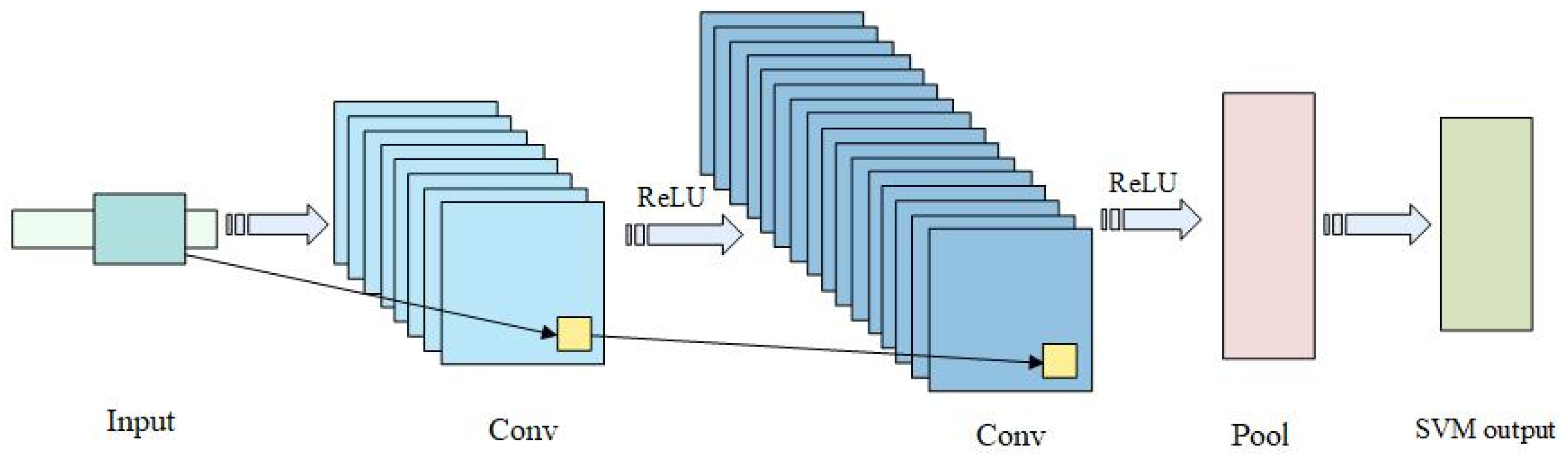
As a powerful deep learning model, the CNN integrates feature extraction and classification recognition, demonstrating significant advantages in signal processing and classification fields while saving time. In recent years, intelligent fault diagnosis algorithms based on CNNs have developed rapidly. Their outstanding advantage is their highly automated feature extraction capabilities, which can directly learn and extract important features from raw monitoring data, reducing the dependence on manual intervention and domain knowledge [7,8]. In low signal-to-noise ratio environments, CNNs can exhibit higher robustness, gradually replacing traditional signal processing methods in natural gas pipeline fiber optic monitoring applications. One-dimensional convolutional neural networks (1D-CNNs), in particular, can effectively balance recognition speed and effectiveness when processing one-dimensional signals. Huang et al. [9] directly input various raw vibration signals into a one-dimensional convolutional neural network for recognition, achieving intelligent fault diagnosis and improving diagnostic accuracy and operational efficiency. Ma et al. [10] used a CNN with multi-scale feature fusion to recognize four types of fiber optic vibration signals, achieving relatively good recognition results. Houdan et al. [11] used a 1D-CNN to extract frequency domain features of fiber optic perimeter signals, showing significant recognition effects for signals with complex frequency components. Li et al. 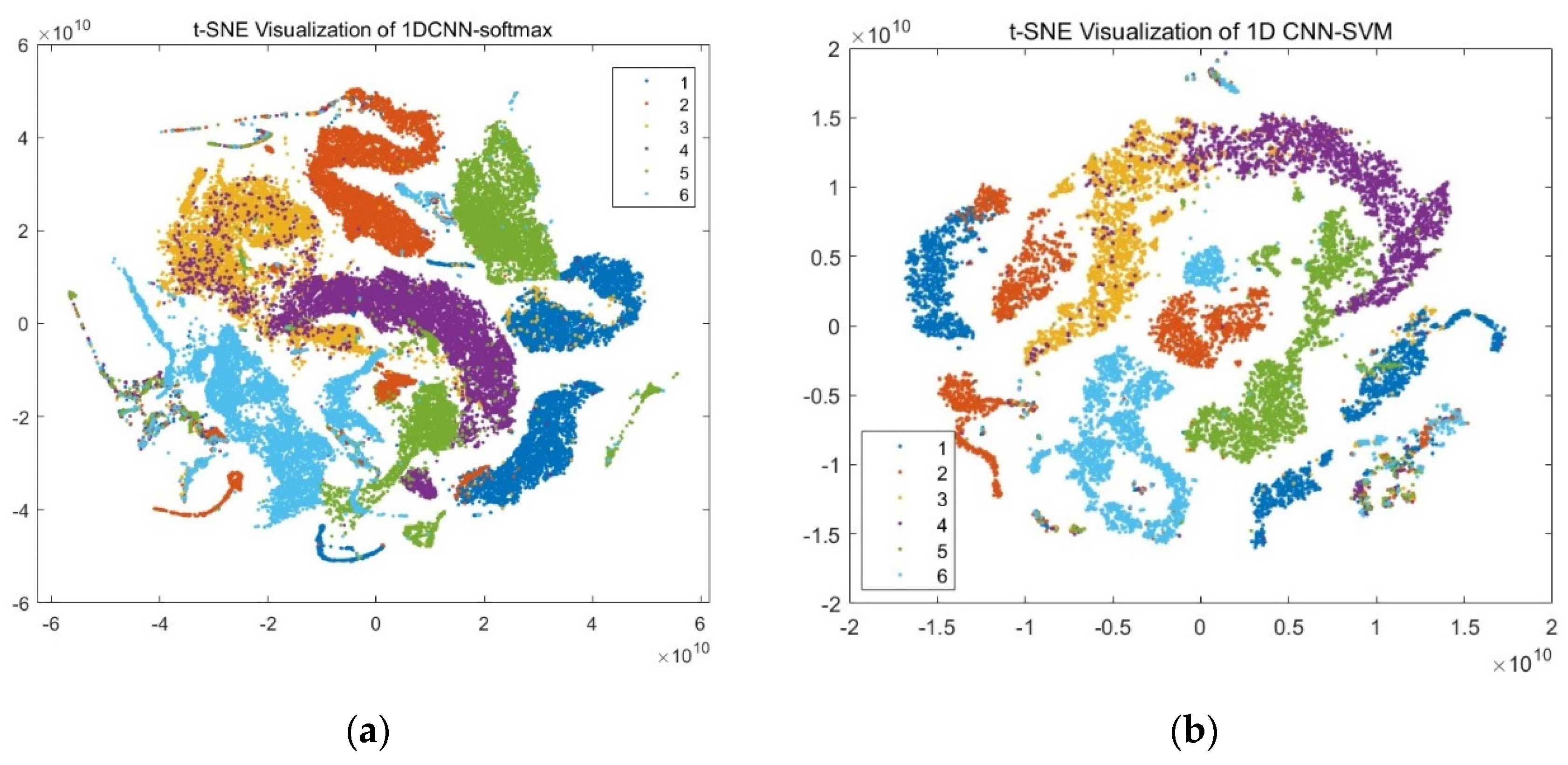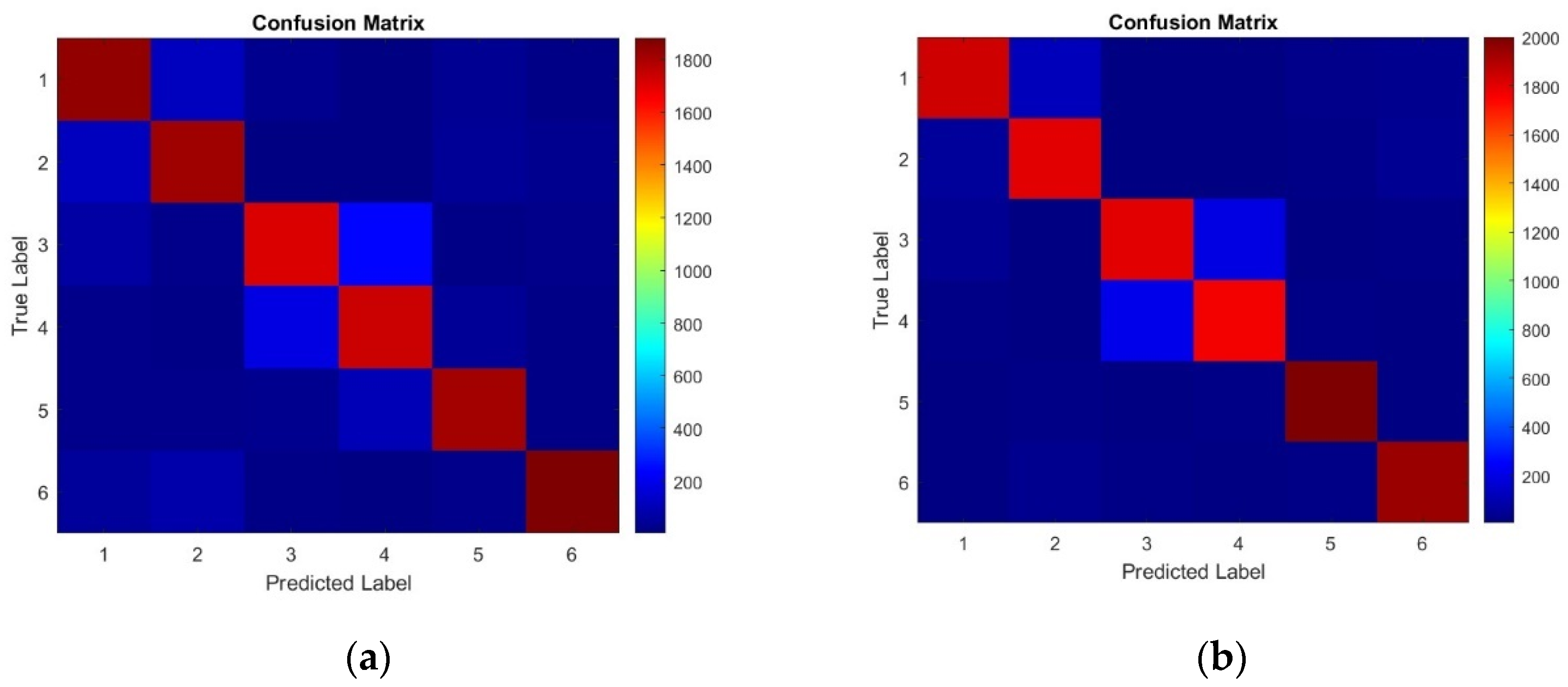[12] implemented electromechanical vibration signal fault diagnosis based on a 1-DCNN, demonstrating good recognition rates, robustness, generalization ability, and noise resistance performance. However, despite the many advantages of convolutional neural networks, they still face some challenges in practical applications. The original data are typically complex and redundant, with a large quantity of noise signals present. Moreover, the signal characteristics generated by different physical vibrations vary significantly, which gives rise to difficulties in classification and processing. This is especially true in complex environments where vibration signals are readily susceptible to interference from external factors. For instance, the vibration signals produced by events like excavator operation, walking, running, impact, theft, and natural gas leakage possess diverse frequencies, amplitudes, and durations. Consequently, traditional vibration signal analysis methods struggle to achieve high-precision classification. Therefore, it is necessary to combine advanced feature extraction algorithms and machine learning technologies to bolster the model’s capacity to discriminate complex vibration features and withstand noise. In 2019, Wu et al. compared classifiers such as softmax, SVM, RF, and XGB and found that the 1D-CNN-SVM combination had the best performance, with an average accuracy rate of over 98% in recognizing five typical DAS signals, significantly outperforming traditional machine learning and 2D-CNN-related deep learning methods [13].

Additionally, when using a 1D-CNN in combination with a Softmax classifier, classification bias may occur due to insufficient samples in certain categories or insufficiently labeled data. At the same time, the process of labeling unlabeled data is both time-consuming and labor-intensive, thereby diminishing the efficiency of data processing [14]. In contrast, few-shot learning [2,3] can achieve rapid learning with a small number of samples when data are limited, greatly improving the learning efficiency and classification accuracy of the model. Existing methods have two main shortcomings:

(1)

Although the 1D-CNN algorithm performs well on large sample datasets [15], it exhibits instability in few-shot learning scenarios, potentially leading to reduced classification accuracy. Most studies mentioned in the literature focus on large-scale datasets, with relatively little research on adaptability and classification accuracy for small sample data.

(2)

SVM demonstrates strong learning ability for small samples and good classification applications [16], but for large-scale datasets, it has high computational complexity and low efficiency. This indicates that while SVM is suitable for small samples, it has high computational complexity for large-scale datasets.

Fiber optic vibration signals are characterized by complexity and high dimensionality, making data preprocessing challenging. For example, one set of data in this study is 10,241 × 1025 in size, which is large, numerous, and extremely complex [17]. The key challenge is how to effectively extract features and reduce data dimensionality while ensuring that classifiers like SVM can maintain high accuracy on small sample data. Therefore, in fiber optic data analysis, it is crucial to focus on optimizing algorithms and data processing techniques to improve the accuracy and efficiency of data analysis [18,19].

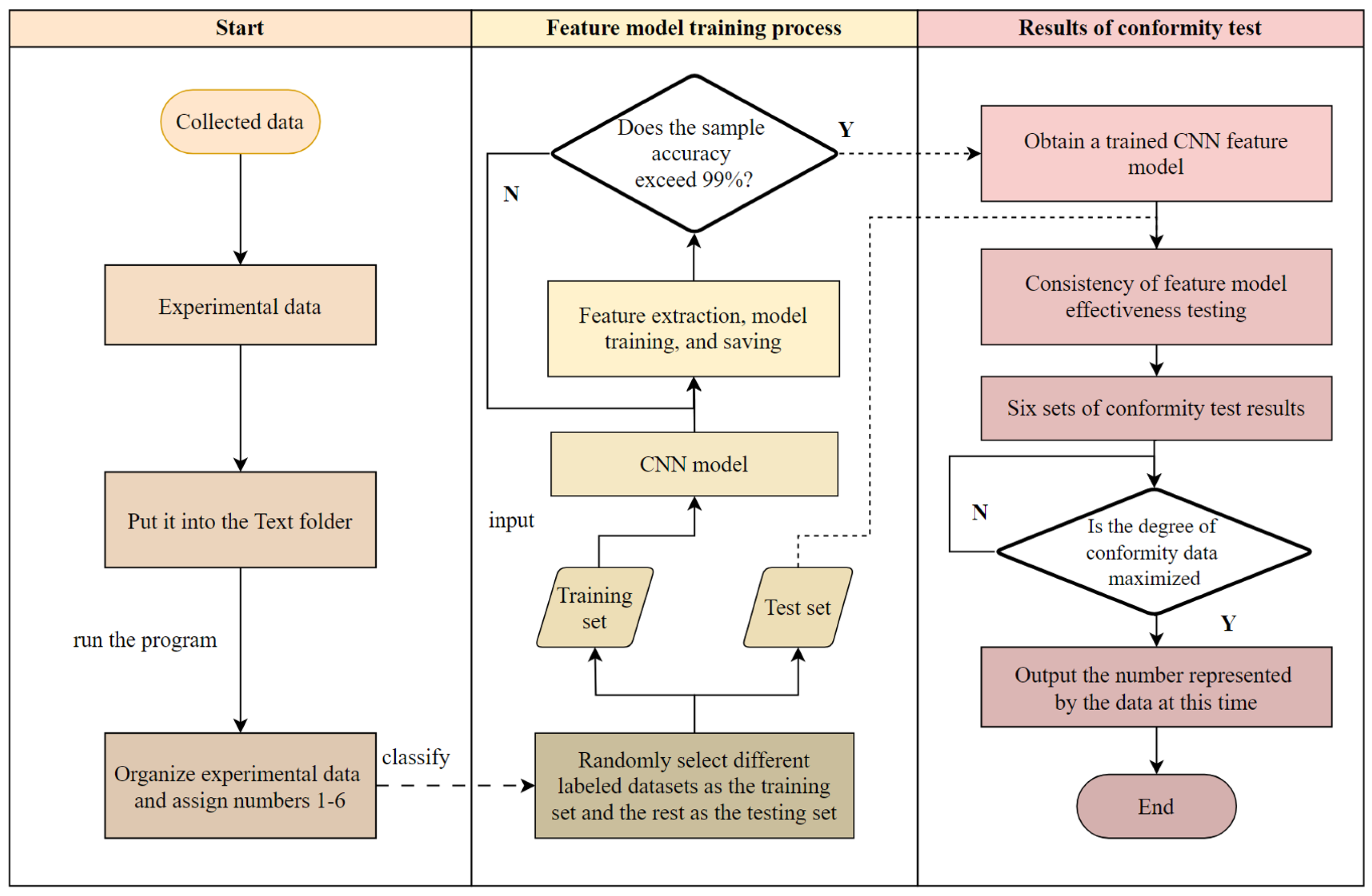
As mentioned above, to address these issues, this paper proposes an improved method combining the 1D-CNN and SVM, utilizing 1D-CNN’s feature extraction capabilities and SVM’s advantage in few-shot learning to achieve accurate analysis and recognition of distributed fiber optic monitoring signals [20]. The proposed approach sustains a high level of classification accuracy even in small-sample scenarios while simultaneously enhancing computational efficiency and model robustness. Experimental evaluations further confirm its reliable performance across a variety of fiber optic vibration signal types, highlighting its strong applicability to natural gas pipeline safety monitoring. These findings offer meaningful insights that may inform the advancement of intelligent pipeline surveillance technologies [21,22]. Although DFOS technologies such as Φ-OTDR have shown great potential in pipeline monitoring due to their real-time and distributed sensing capabilities, most existing studies still rely on conventional feature engineering and classifiers, which limits adaptability under complex environments. Although deep learning techniques have gained traction in recent years, their performance tends to decline in small-sample contexts due to overfitting and limited generalization. To address this limitation, combining the automated feature extraction capability of a 1D-CNN with the strong classification efficacy of an SVM under sparse data conditions offers a promising pathway for improving the practical interpretation of distributed fiber optic sensing (DFOS) data in complex real-world environments.

1.3. Comparative Advantages

Existing studies, such as [13,23], have explored CNN-based models for pipeline monitoring, but key limitations remain. A comparative analysis of our method with these works is summarized in

Table 1. Comparison of 1D-CNN-based methods for natural gas pipeline monitoring.

Comparison Dimension	This Method (1D-CNN-SVM)	Reference [23] (1D-CNNs-BiLSTM)	Reference [13] (1D-CNN)
Application Domain	Safety monitoring of natural gas pipelines (quantification of leakage sizes and distinction of mechanical vibrations)	Distributed fiber optic acoustic sensing (DAS) signal classification (five types of events)	Pipeline monitoring (vibration recognition)
Adaptation to Signal Characteristics	Optimized for high noise, multimodality, and small-sample conditions in DFOS	Not explicitly targeted at high-noise or small-sample scenarios	Relies on traditional feature engineering, with no mention of noise robustness
Classifier Design	SVM (addresses class imbalance and enhances feature discrimination in small samples)	Softmax (does not specifically address imbalance issues)	Softmax (does not specifically address imbalance issues)
Real-Time Performance	0.819 ms latency, meeting industrial-level real-time monitoring requirements	Real-time performance metrics not mentioned	Real-time performance metrics not mentioned

.

This table compares the differences between the method in this paper (1D-CNN-SVM) and those in references [23] (1D-CNNs-BiLSTM) and [13] (1D-CNN) across four dimensions. It highlights the advantages of this method in the quantitative monitoring of natural gas pipeline leaks, classification accuracy for small samples, noise resistance, and industrial-grade real-time performance.

2. Materials and Methods

2.1. DAS3000 System

Distributed optical fiber sensors are a type of fiber-based sensor technology that uses optical fibers as the sensing element, capable of measuring or monitoring spatial distribution and spatio-temporal variation information along the optical fiber transmission path. By deploying sensing fibers in the measurement field, the sensors can determine real-time spatial characteristics and dynamic changes in the measured environment. Distributed optical fiber monitoring technology achieves safety and early warning by capturing vibration signals around pipelines in real time, but the original signals face challenges of high noise and complex multimodal features [8,24]. Traditional methods rely on manual feature engineering, such as wavelet transform (WT) and empirical mode decomposition (EEMD), which are inefficient and insufficiently adaptive to complex scenarios [24,25]. Recently, there has been growing interest in applying deep learning models to this area of research due to their automatic feature extraction capabilities. For example, in motor fault diagnosis, 1D-CNN extracts time-series features through convolutional and pooling layers and achieves an identification accuracy of 99.91% after optimizing parameters with the Taguchi method, significantly outperforming traditional algorithms [8]. Similarly, in the corona fault detection of switchgears, the 1D-CNN-LSTM hybrid model achieves 100% classification accuracy in frequency-domain analysis, verifying the effectiveness of combining convolutional neural networks with recurrent networks [24].

When construction equipment operates near the optical fiber, it generates vibration waves. These waves transmit vibration signals to nearby fiber optic cables, causing synchronous vibrations in the fibers within the cable. This leads to micro-deformations in the fiber, resulting in changes to the polarization state of the optical signal within the fiber. Consequently, the local refractive index also changes, causing the incident light passing through this area to produce scattered light. The DAS3000 system (Hangzhou Optosensing Co., Ltd., Hangzhou, China) detects and analyzes this scattered light, and through analysis of this information, the vibration data of the fiber can be obtained. This is illustrated in Figure 1.

Schematic of the measurement principle of the DAS3000 system. The system utilizes a narrow-linewidth distributed feedback (DFB) laser as the light source. An electro-optic modulator (EOM) modulates the laser pulses, which are then amplified by an erbium-doped fiber amplifier (EDFA) and injected into the sensing fiber. External vibrations (e.g., from construction equipment) cause phase changes in the backscattered Rayleigh light, which is detected and analyzed using coherent detection and real-time signal processing. EOM: Electro-optic modulator; EDFA: Erbium-doped fiber amplifier.

However, the original data are complex and redundant. Different physical vibrations generate signals with distinct characteristics, and there is also noise present. Consequently, it is necessary to utilize algorithms to extract the features of the original signals for alarm determination and to classify the monitoring signals based on their signal features. In this study, a narrow-linewidth distributed feedback (DFB) laser was employed as the light source. The laser pulses were modulated by an electro-optic modulator (EOM), amplified by an erbium-doped fiber amplifier (EDFA), and injected into the single-mode sensing fiber. Coherent detection was adopted for capturing Rayleigh backscattering signals. All abbreviations, including EOM and EDFA, are defined at their first occurrence.

Figure 2 illustrates the workflow for processing fiber optic vibration data using the proposed method. The process consists of several key stages, outlined as follows: experimental system and data collection (the image in the data acquisition box reflects the result of collecting the entire line.), 1D-CNN model training, feature extraction, and data processing. The details of each step will be discussed in the following sections.

2.2. Experimental System and Data Collection

The machine employed in this article is the distributed optical fiber vibration sensing system DAS3000 of Hangzhou Optosensing Co., Ltd. (Hangzhou, China), as shown in Figure 3a. The hardware environment consists of a 64-bit Windows 11 operating system, with a 13th Gen Intel(R) Core (TM) i7-13650HX processor running at 2.6 GHz, 16 GB of memory, and a 1 T solid-state drive. The system parameters set for data collection during the experiment are as follows: alarm duration of 10 s, data collection delay time of 10 s, short-distance optical module type, EDFA current of 150 mA, and Unl (unlabeled or auxiliary laser driving current for system calibration, as defined in the DAS3000 system documentation) current of 120 mA. The measurement parameters are 5 KM, the sampling frequency during data collection is 6000 Hz, the sampling rate is 100 MHz, the sampling interval is 1 m, the spatial resolution is 10 m, the measurement channel is 1, the fiber refractive index is 1.468, and the attenuation coefficient is 0.15. The optical fiber used in this experiment is a single-mode G652 metal spiral armored optical cable(Hengtong Optic—Electric Co., Ltd. Suzhou, Jiangsu, China) with a diameter of 3.0 mm, PVC sheath, and a length of 1 km, as shown in Figure 3b. The sensing cable used was a single-mode G652 metal spiral armored optical cable with a 3.0 mm diameter and a polyvinyl chloride (PVC) outer sheath. The data are collected using a co-laying method with the gas pipeline.

Figure 4 shows the optimized 1D-CNN structure. From left to right, the input layer (Input) receives data first. Then, there are two convolutional layers (Conv), which extract features through filters, with the small yellow squares representing the filters. After each convolutional layer, there is a ReLU activation function to introduce nonlinearity. Next comes the pooling layer (Pool), which is used to reduce the data dimension. Finally, there is the support vector machine (SVM) output layer, which is used to classify the extracted features.

We conducted an on-site trial at a gas station in Quzhou City, Zhejiang Province, where the fiber optic cable was co-laid with the natural gas pipeline under real environmental conditions to ensure signal authenticity and variability; in order to obtain the correct data, we examined the laying situations of the optical cable and the pipeline and checked whether the instrument displays were normal. The DAS3000 system collects vibration signals around the gas pipeline in real-time. When vibration occurs, the DAS3000 system automatically records the relevant alarm data and generates a series of h5 format files with dimensions of 10,421 × 1025. After systematically collecting and organizing these data, a thorough analysis was conducted to evaluate the vibration characteristics and potential risks of natural gas pipelines.

2.3. Hybrid Algorithm Framework

This paper adopts an improved method combining 1D-CNN and SVM, utilizing 1D-CNN’s automatic feature extraction capabilities and SVM’s advantage in few-shot learning to achieve precise analysis and recognition of distributed fiber optic monitoring signals [20].

The architecture shown in Figure 4 was selected after preliminary testing of several CNN-based configurations. Initial models using standard 1D-CNN combined with Softmax classifiers showed limited performance when handling class imbalance and small-sample conditions, particularly for minority events such as pipeline leakage. Furthermore, fully connected layers combined with Softmax tended to overfit when training data were insufficient or noisy.

To mitigate the aforementioned issues, a streamlined architecture was adopted, incorporating shallow one-dimensional convolutional layers combined with max pooling and dropout operations. This configuration facilitates stable extraction of low-level features while effectively limiting overfitting. In contrast with conventional approaches utilizing Softmax classifiers, a multi-class support vector machine (SVM) was employed as the final classification layer, leveraging its margin-maximization capabilities, which are particularly advantageous under limited sample conditions. This integration of CNN-based feature learning with SVM’s robust generalization capacity yielded a hybrid model that achieved superior performance. Experimental validation (see Section 3.3) confirmed that the proposed architecture enhanced average classification accuracy by 2.03% and improved feature separability by 19.7% compared to the baseline CNN-Softmax framework, thereby supporting its suitability for complex signal classification tasks.

These findings are in line with prior research on shape memory alloy (SMA) actuator position estimation, whereby 1D-CNN architectures—when structurally optimized through techniques such as dropout—demonstrated a favorable trade-off between computational efficiency and generalization, particularly under small-sample constraints. Notably, inference speed was reported to be 1.26 times faster than that of LSTM networks [10]. Similarly, in the task of multi-class missile classification based on radar cross section (RCS) signals, a 1D-CNN-GRU hybrid model incorporating four convolutional layers and gated recurrent units attained 99.5% accuracy under noisy conditions, further supporting the model’s robustness in complex signal environments [25].

2.3.1. Convolutional Neural Network

The CNN is a class of deep learning neural networks primarily used for processing grid-structured data, images, and videos. The most common structure of a CNN includes convolutional layers, pooling layers, fully connected layers, as well as nonlinear activation functions and loss functions. The typical format involves stacking convolutional layers and activation layers (ReLU layers), followed by pooling layers (aggregation layers), repeating this pattern until the image is spatially reduced to a sufficiently small size, with the final fully connected layer producing the output. It is modeled after the biological visual perception mechanism and can perform both supervised and unsupervised learning. The parameter sharing of convolutional kernels in its hidden layers and the sparsity of inter-layer connections enable CNNs to extract gridded features with relatively low computational cost. A 1D-CNN is mainly used for processing one-dimensional sequence data. Compared to traditional fully connected neural networks, a 1D-CNN can utilize convolutional kernels to automatically learn the internal relationships between sensor data in the sliding direction, extracting effective features related to the monitoring signal. This paper combines the advantages of SVM in few-shot learning to achieve rapid recognition and high-precision classification of optical cable vibration signals.

The convolutional layer convolves a 1D convolutional kernel with a one-dimensional input signal, and local features can be extracted through the activation function in the convolutional layer. The following formula is the mathematical expression of the convolutional layer in a convolutional neural network, demonstrating how new features can be generated through the computation of convolution and bias terms:

$$x_l^j={\sum }_{i=1}^n\mathrm{c}\mathrm{o}\mathrm{n}\mathrm{v}({\omega }_{ik}^{j-1},s_i^{j-1})+b_l^j$$

(1)

In the formula, $x_l^j$ represents the $j$-th feature map at the $i$-th layer; $n$ means the number of input features; ${\omega }_{ik}^{j-1}$ is the weight parameter of the $k$-th convolutional kernel (filter) at the $j-1$-th layer; $s_i^{j-1}$ is the $i$-th input feature map at the $j-1$-th layer; and $b_l^j$ is the bias term corresponding to the $j$-th feature map at the $l$-th layer.

The vibration signal features of fiber optic warning events extracted through convolutional layers are introduced into the pooling layer to preserve useful features and reduce unnecessary features, making the extracted features more reflective of different types of fiber optic vibration. This article adopts the maximum pooling operation, and the formula is as follows:

$$z_k^{j(\alpha )}=\underset{(\alpha -1)r+1\le \beta \le \alpha r}{\max }\left\{y_k^{j(\beta )}\right\}$$

(2)

In the formula, $z_k^{j(\alpha )}$ is the output of the operation at the $k$-th position for the $j$-th feature map at the $\alpha$-th layer; $\beta$ is an index variable used for the maximum operation; $r$ is a pooling size or a stride parameter; and $y_k^{j(\beta )}$ represents the input values to the pooling operation at the $k$-th position for the $j$-th feature map at the $\beta$-th layer.

This article chooses ReLU as the activation function, which provides a simple nonlinear judgment and helps solve the problem of gradient vanishing in neural networks to avoid overfitting [26]. The formula is as follows:

$$f\left(z\right)=\left\{\begin{array}{l}zz>0\\ 0z\le 0\end{array}\right.$$

(3)

The 1D-CNN has a filter size (in this case, it is 3), a stride (which determines the sliding step size of the filter), and a number of filters. The pooling layer has a pooling window size and stride. The fully connected layer has a number of neurons, weights, and biases. The fully connected layer no longer extracts features, but instead combines the extracted features and maps them to the sample label space. The SVM classifier performs a nonlinear or linear transformation on the data based on the type of its kernel function and combines the penalty parameter to balance model complexity and the training error, ultimately outputting the classification result.

2.3.2. Support Vector Machine

SVM was first proposed by VAPNIK in 1995. This method is a learning approach that uses structural risk minimization criteria. Compared to traditional learning methods that use empirical risk minimization criteria, SVM has stronger generalization ability and is widely used in statistical classification and regression analysis [20]. Firstly, it finds the points closest to the separating hyperplane and then ensures that these points are as far away from the separating surface as possible. The distance from the points to the separating surface doubled is called the margin, and the support vectors are the points closest to the hyperplane. For the nonlinear training samples input $Z\in \left\{(x_i,y_i)\right\}(i=1,2,\dots ,N)$, where $x_i$ is the input feature of SVM, $y_i$ is the corresponding label of the input feature, and $N$ is the number of input features. The mathematical model of the optimization problem of the hyperplane for nonlinear sample classification is as follows:

$$\max \left\{{\displaystyle \frac{1}{2}}{‖\omega ‖}^2\right\}+B{\displaystyle \sum _{i=1}^n{\xi }_i}$$

(4)

The constraint conditions are as follows:

$$y_i(\omega x_i+a)\ge 1-{\xi }_i,i=1,2,\cdots ,N$$

(5)

$${\xi }_i\ge 0, i=1,2,\cdots ,N$$

(6)

Among them, $\omega$ is the normal vector of the hyperplane; $\xi$ is for relaxation variables; $a$ is the offset of the hyperplane; and $B$ is a penalty factor; it is generally greater than 0, and the larger the value, the greater the punishment for misclassified samples, and the higher the accuracy of training samples, but the model’s generalization ability decreases. The optimal classification decision function obtained by using the Lagrange Multiplier Method is as follows:

$$f(x)=sign\left[{\displaystyle \sum _{i=1}^N{a_i}^{*}{y}_i}T(x_i,y_i)+b^{*}\right]$$

(7)

Among them, ${a_i}^{*}$ and $T(x_i,y_i)$$b^{*}$ are Lagrange multipliers and kernel functions.

The one-dimensional convolutional neural network structure built in this paper is shown in

Table 2. ID-CNN-SVM structure table.

Module	Component	Configuration	Description
Data Input	Data Directory	signal/	Contains multi-class vibration CSV files.
	Class Detection	Auto-scan subfolders	Extracts class labels (labelNames).
Preprocessing	Data Reshaping	reshape ([1 × M × 1 × N])	Adapts raw data to network input dimensions.
	Data Split	cvpartition (80:20)	Stratified sampling to preserve class ratios.
Network Architecture	Input Layer	imageInputLayer ([1 × M × 1])	Accepts 1D vibration signals.
	Convolution Block 1	Conv2d ([1 × 3], 8) + BN + ReLU	Local feature extraction.
	Pooling Layer	MaxPooling2d ([1 × 2], stride [1 × 2])	Downsampling for dimensionality reduction.
	Convolution Block 2	Conv2d ([1 × 3], 16) + BN + ReLU	Deep feature extraction.
	Regularization	Dropout (0.1)	Prevents overfitting.
	Classification Head	FC + Classification	Outputs class probabilities.
Training Config	Optimizer	Adam (lr = 0.0001)	Adaptive learning rate optimization.
	Regularization	L2 (λ = 0.001)	Weight decay for model robustness.
	Validation Strategy	Every 30 iterations + Early Stopping	Monitors overfitting.
Feature Extraction	Deep Features	fc layer activations (16-D)	Extracted features for SVM classification.
Classifier	Multi-class SVM	fitcecoc(default kernel)	Replaces the native network classification head.

. Both convolutional layers use the same step size while keeping the output size unchanged.

2.4. Evaluation Index

In order to verify and evaluate the effectiveness of the proposed method, commonly used performance indicators such as macroscopic accuracy and precision were employed in this study. Macro precision refers to the precision calculated separately for each category, followed by arithmetic mean calculation for all categories [27]. The formula is shown in Formula (8), where accuracy represents the proportion of correctly classified samples to the total sample size. The formula is shown in (9):

$$\mathrm{Precision}={\displaystyle \frac{TP}{TP+FP}}$$

(8)

Accuracy = (TP + TN)/(TP + TN + FP + FN)

(9)

In the formula, TP (True Positive) represents the number of correctly predicted positive values; TN (True Negative) represents the number of correctly predicted negative values; FP (False Positive) represents the number of incorrectly predicted positives; and FN (False Negative) represents the number of incorrect predictions that are negative.

In a multi-class classification task, the average accuracy for each class can be calculated. First, calculate the accuracy for each individual class and then find the average of these class-specific accuracies to obtain the overall average accuracy. Let $a_i$ be the accuracy of the $i$-th class, then the formula for the average accuracy is as follows:

$$Average Accuracy={\displaystyle \frac{{\displaystyle {\sum }_{i=1}^n{a}_i}}{n}}$$

(10)

In the formula, the accuracy of the $i$-th class $a_i={\displaystyle \frac{c_i}{n_i}}$, $c_i$ is the number of samples of the $i$-th class that are correctly predicted, and $n_i$ is the total number of samples in the $i$-th class.

2.5. Data Processing Process

To acquire relatively comprehensive characteristics of the signal, the data was input into the CNN model for training. Firstly, the standard vibration data was categorized by labels. For each event type, 30 data sets were extracted as the training set, and the remaining data sets constituted the test set. Subsequently, feature model training was conducted. By means of MATLAB (Using the educational account and MATLAB Online.), the local features of the fiber alarm data were extracted from the standard data training set via the convolutional and pooling layers of the CNN. These features were then combined and abstracted into high-level features and input into the SVM classifier. The SVM model was trained until the highest accuracy was attained. The model parameters during training were utilized to transfer the test set data to the model for classifying the vibration types of the fiber alarm data into the feature library. The training set was input to extract the features related to fiber vibration, followed by the output of the extracted features through the fully connected layer and their transmission to the output layer. In the output layer of the 1D-CNN, the SVM classifier was utilized to replace the conventional softmax classifier to further enhance the classification accuracy and obtain distinct data features. Eventually, based on the conformity test, the feature number with the greatest degree of conformity was identified as the data type, facilitating the classification of the experimental data. Similarly, in the classification of optical fiber vibration signals, the 1D-CNN-SVM hybrid model extracts frequency-domain features of vibration waveforms through convolutional layers and utilizes the margin maximization property of SVM to effectively distinguish similar signals such as “walking/running” and “excavator operation”. Such hybrid architectures demonstrate stronger feature representation capabilities in multi-source data fusion scenarios [11,13]. The flow chart of experimental data processing is shown in Figure 5.

3. Results and Discussion

3.1. Sample Construction

The data used in this paper were monitored using the DAS3000 system. There are six types of data in total: 1 mm pipeline leakage, 3 mm pipeline leakage, 5 mm pipeline leakage, impact theft, excavator operation, and walking/running.

Furthermore, this paper labels these six types of data with corresponding event tags: 1 mm leakage—1; 3 mm leakage—2; 5 mm leakage—3; impact theft—4; excavator operation—5; walking/running—6. The size of the established total training database is shown in

Table 3. Classification of event type labels.

Types of Data	Dataset	Label
1 mm leakage	1,095,573	1
3 mm leakage	1,075,095	2
5 mm leakage	1,064,856	3
Impact theft	1,013,661	4
Excavator operation	1,034,139	5
Walking/Running	1,044,378	6

.

Based on the alarm logs and changes in signal intensity, the approximate location of the event occurrence could be inferred. The alarm signals were then denoised, and the normalized alarm data were stored as a 10,241 × 1025 h5 data format file, which means that one dataset contains 10,241 pieces of data, and 1025 represents the data of intensity changes along the entire optical fiber recorded at one time. The collected data ensures that the entire event is fully captured, covering both the start and end of the event. The alarm signal images for each type of event can be referenced in Figure 6. The figure displays a waterfall plot of distributed optical fiber monitoring data. The horizontal axis indicates the number of sampling points (corresponding to distance, unit: m). The left vertical axis represents the sequence number of data samples, used to identify the chronological order of different data records. The color bar on the right vertical axis is labeled “×10⁴”, ranging from blue to red with values from 0 to 3 × 10⁴, indicating the magnitude of values corresponding to different colored regions in the plot. This color bar serves as a visual key to interpret the color mapping in the figure, where colors intuitively reflect the relative intensity levels of the physical quantity (energy amplitude [a.u.]) across different regions.

From Figure 6, signal energy is primarily concentrated in the left-side near-100 region of the horizontal axis, with a large low-energy blue feature dominating the right side. This distribution pattern indicates that the measured physical quantity exhibits significant response characteristics at the pipeline’s proximal end.

Regarding specific signal patterns: Leakage signals (1 mm/3 mm/5 mm) and mechanical excavation signals (Figure 6a–c,e) show similar red-yellow distributions in the left high-energy zone, but differences in stripe morphology and color gradients distinguish leakage aperture and mechanical operation features. Leakage signals exhibit a bimodal structure (narrower peak spacing for smaller apertures), while mechanical signals show a single main peak with rapid secondary peaks.

The impact theft signal (Figure 6d) displays a unique compact high-intensity distribution, with significantly higher energy concentration than other types. This “steep peak-rapid decay” pattern likely corresponds to the physical characteristics of instantaneous impacts.

Walking/running signals (Figure 6f) are characterized by vertically extended orange-yellow distribution bands, reflecting the continuous spatio-temporal propagation of broadband vibrations from human activities.

These differences fundamentally reflect the mechanisms of different excitation sources: frequency dispersion in leakage signals related to fluid dynamics, periodic impacts in mechanical vibrations, and broadband continuous vibrations from human activities. These waterfall plots provide a theoretical basis for the identification and classification of abnormal pipeline behaviors.

3.2. Feature Extraction

Approximately 70% of the sample data were selected as input for training the hybrid model, with the remaining 30% used to test the fault recognition performance of the trained model. The accuracy curve and loss curve of the test set are shown in Figure 7.

When filters perform convolution operations on input data, they output a new two-dimensional array called a feature map. The feature map expresses the locations of specific types of features detected by the filter in the input data. Feature maps are generated through convolution operations between filters and input data, with each feature map reflecting the input data’s response when the filter detects certain specific features. In simple terms, filter weights determine the type of features to be detected, while feature maps show the spatial distribution of these features in the input data. In the first convolutional layer of the 1D-CNN, the interaction between the filter weights and the feature maps of a specific image serves as the starting point for the entire network to carry out feature extraction. Through this interaction, the network starts to explore and extract potentially useful features from the raw data. These features might be the edges of the data, which provide a foundation for the subsequent convolutional layers to further extract higher-level features and for final task processing. The interaction between the filter weights of the first convolutional layer and the feature maps of the image will extract the basic characteristics of the data, providing clues for the subsequent identification of the data type. The filter weights of the first convolutional layer after training are shown in Figure 8a, and the feature map of a specific image after the first convolutional layer is shown in Figure 8b.

As feature maps do not express features clearly and are not easily observable by the human eye, the T-SNE (T-Stochastic Neighbor Embedding) visualization technique is used to reduce the features of the 1D-CNN-softmax and 1D-CNN-SVM models to two dimensions and visualize them through plotting. The features are represented as the output of the last classification layer. The visualization results are shown in Figure 9, where it can be clearly seen that after replacing the Softmax classifier with SVM, the distribution of various features becomes more distinct. We applied T-SNE (T-distributed Stochastic Neighbor Embedding) to reduce the high-dimensional feature vectors extracted by the 1D-CNN to two dimensions for visualization of feature separability. A proper implementation and theoretical foundation for T-SNE can be found in (van der Maaten & Hinton, 2008) [28]

Then, the confusion matrices of the two methods in a random test are shown in Figure 10. The results indicate that the proposed method (1D-CNN-SVM) performs better than the traditional machine learning method (1D-CNN-Softmax) as illustrated in Figure 10a and b, respectively. After the above verification, the extracted features are proven to be effective and significantly different. At this point, we can use these features to validate signal classification in actual construction operations.

3.3. Data Classification Analysis

The training set data were processed using both 1D-CNN-softmax and 1D-CNN-SVM for training and feature extraction. Based on the model results, and to maintain generality, a comparative analysis with the Transformer architecture was conducted; the model was subjected to five repeated experiments, with the average taken. The experimental results and data validation compatibility were calculated using Formula (8), as shown in

Table 4. Comparison of test results of the different models.

Model	Event Type 1	Event Type 2	Event Type 3	Event Type 4	Event Type 5	Event Type 6
1D-CNN-softmax	0.90565	0.92987	0.84323	0.42768	0.60312	0.80243
Transformer	0.90542	0.93513	0.86689	0.86807	0.96759	0.95802
1D-CNN-SVM	0.91667	0.93143	0.87184	0.96469	0.95722	0.97901

and illustrated in Figure 11.

According to the Formula (10), the 1D-CNN-softmax model algorithm achieved an average accuracy of 0.75199, while the Transformer model yielded an average accuracy of 0.91685, demonstrating more balanced performance that surpassed the 1D-CNN-softmax model but fell short of the improved 1D-CNN-SVM model. The 1D-CNN-SVM model algorithm produced an average accuracy of 0.93681, representing an improvement of 19.7%.

Twenty sets of data were randomly extracted from the test set and input into the program using the recently extracted 1D-CNN-SVM feature model. The data validation compatibility, calculated according to Formula (9), is shown in

Table 5. The degree of correspondence of event type features in the validation set.

Number	Event Type 1	Event Type 2	Event Type 3	Event Type 4	Event Type 5	Event Type 6
1	0.82959	0.01093	0.12842	0.00815	0.00830	0.00947
2	0.00351	0.00234	0.00585	0.01015	0.87629	0.00595
3	0.00917	0.00244	0.04306	0.91074	0.19102	0.00947
4	0.13789	0.00234	0.23223	0.79736	0.00634	0.01582
5	0.01971	0.13545	0.05389	0.10276	0.81865	0.18653
6	0.10139	0.09581	0.05706	0.81734	0.11929	0.07197
7	0.01813	0.80819	0.12758	0.03220	0.10551	0.11084
8	0.05784	0.18143	0.10997	0.04937	0.01386	0.81989
9	0.08644	0.09326	0.01001	0.79118	0.01374	0.01764
10	0.06351	0.90664	0.01083	0.11106	0.17385	0.01958
11	0.00802	0.05265	0.90950	0.01941	0.00488	0.01629
12	0.01090	0.01511	0.01742	0.01661	0.71051	0.85294
13	0.00733	0.11046	0.81966	0.05105	0.17776	0.09147
14	0.06225	0.02100	0.13420	0.07238	0.90264	0.01491
15	0.1527	0.03611	0.07088	0.70687	0.15564	0.00199
16	0.01247	0.01436	0.15529	0.20588	0.17091	0.81465
17	0.80637	0.05606	0.09881	0.07344	0.17495	0.10660
18	0.00143	0.80148	0.17916	0.18023	0.14865	0.03206
19	0.19783	0.08114	0.80747	0.15942	0.06977	0.02076
20	0.08097	0.03391	0.20478	0.01976	0.82036	0.18023

.

Table 5 shows that the data with ID 1 have the highest compatibility (0.82959) with the features of event type 1, indicating that these data corresponds to a 1 mm leak event. It can be observed that the validation set has a high response compatibility with the extracted features, allowing for significant differentiation from other data type feature responses, thus enabling clear determination of the data type.

The alarm signals of construction equipment operations extracted by DAS3000 from the line were input into the program, totaling 208 sets. Using the Formula (9), the classification accuracy data after feature value validation performed by the two different 1D-CNN models on the experimental set are shown in

Table 6. Experimental data verification and corresponding accuracy.

Sample Labels	Number of Samples/Number of Samples			Accuracy
	Actual Quantity	1D-CNN Softmax Verification Quantity	1D-CNN-SVM Verification Quantity	1D-CNN-Softmax	1D-CNN-SVM
1	204,780	204,780	204,780	100%	100%
2	215,019	194,541	214,108	90.47%	99.57%
3	143,346	143,346	143,346	100%	100%
4	368,604	368,604	368,604	100%	100%
5	563,145	563,145	563,145	100%	100%
6	634,818	655,296	635,129	96.87%	99.95%

.

After validation with the 1D-CNN-softmax feature algorithm, as the Formula (10), the average accuracy reached 97.89%. However, after validation with the 1D-CNN-SVM feature algorithm, the accuracy improved to 99.92%. The classification accuracy increased by 2.03% after replacing the softmax classifier with SVM. Observing Figure 6, it was found that the one-dimensional signal graphs of sample labels 2 and 6 have similar shapes after reaching the second peak. Further analysis showed that event type 6 had the most alarm occurrences, while event type 3 had the least. Overall, leak alarms were less frequent, while walking and running triggered more alarms, followed by excavator operations. This indicates that vibration signals were mainly caused by construction site activities, and timely judgment of vibration types can reduce potential hazards to natural gas pipelines from construction sites and improve safety awareness. Additionally, the algorithm achieved 100% recognition rates for data categories 1, 3, 4, and 5. Observing Figure 6, it was found that under conditions of smaller vibration amplitudes, the one-dimensional signal graphs of sample labels 2 and 6 have relatively similar shapes after reaching the second peak, occasionally resulting in misjudgments.

Overall, the features derived from the training dataset proved to be both reliable and informative. Experimental data validation shows that the overall recognition accuracy is generally above 90%. Validating 10,241 sets of data takes only 8.39 s, with an average processing time of 0.000819 s per alarm signal, meeting the requirements for real-time data type recognition. Compared with the baseline methods in the public Φ-OTDR dataset [2], the method in this paper improves the F1-score by 11.2%. This demonstrates that the feature signals extracted based on the 1D-CNN-SVM algorithm are fast and accurate in fiber optic cable monitoring and recognition for external damage prevention. This can significantly reduce labor costs, promote the intelligence of fiber optic early warning systems, and enhance the system’s effectiveness in pipeline safety protection.

In general, leak-related events accounted for a smaller proportion of alarms, whereas human activities such as walking and running generated more frequent alerts, with excavator operations ranking next. This trend suggests that the majority of vibration signals are closely associated with construction-related disturbances. Such insights help refine the focus of monitoring efforts and enhance the effectiveness of early warning strategies. Leveraging the pattern recognition capabilities of the 1D-CNN-SVM model, the DAS3000 system demonstrates improved accuracy in detecting pipeline anomalies, thereby supporting proactive interventions aimed at maintaining infrastructure stability and ensuring the continuous functioning of surrounding socio-economic systems.

4. Conclusions

This study proposes a fiber optic vibration event recognition method based on the combination of a one-dimensional convolutional neural network (1D-CNN) and a support vector machine (SVM). By collecting data with the DAS3000 distributed vibration sensing system, this paper successfully combines the automatic feature extraction capabilities of 1D-CNN with the few-shot learning advantage of SVM, achieving efficient classification of fiber optic vibration signals. In practical experiments, the average correct recognition rate of 1D-CNN-SVM reached 99.92%.

In the tested environment (Intel i7-13650 HX, 16 GB RAM), the 1D-CNN-SVM algorithm demonstrated outstanding real-time performance: a single-signal processing latency of merely 0.819 ms and a theoretical throughput of 1221 signals/second. Compared with the conventional 1D-CNN-Softmax approach (1.2 ms latency, 833 signals/second throughput), the SVM classifier reduced the response time by 31.7%. Notably, no significant latency accumulation was observed during simulated continuous data stream processing (100,000 signals), fully meeting real-time monitoring requirements.

Our experimental findings demonstrate that the proposed 1D-CNN-SVM algorithm delivers robust performance characterized by both low latency and high throughput. In the context of natural gas pipeline monitoring, the model achieved a high classification accuracy of 99.92% in detecting critical events such as leakage and mechanical excavation. Through automated feature extraction and efficient classification, the system substantially reduces reliance on manual inspection—cutting false alarm rates by more than 90%—and lowers potential safety risks to below 0.1%. Beyond algorithmic advancements, this research bridges the gap between theory and application by embedding the model into operational workflows of gas station monitoring systems.

By enabling the timely and accurate transmission of critical alerts to inspection personnel, the system has notably enhanced the overall safety management practices at monitored facilities. As such, it offers a practical and scalable solution for safeguarding natural gas transmission infrastructure and establishes a solid groundwork for the broader deployment of fiber optic sensing technologies in related engineering fields.

Existing studies demonstrate that 1D-CNN and its hybrid models exhibit superior performance in time-series signal tasks such as pipeline monitoring and fault diagnosis, particularly in scenarios involving small samples and multimodal data. Future research could further explore lightweight designs (e.g., model compression and quantization) to adapt to edge devices [10] or incorporate attention mechanisms to enhance the weighting of critical features [25]. Additionally, integrating physical prior knowledge (such as the principles of fiber optic sensing) to optimize network architectures is expected to further improve generalization capabilities in complex environments [26]. Future research can continue to optimize this method, further improving the algorithm’s generalization ability and computational efficiency on larger-scale datasets and exploring its potential applications in other complex environments.

References

1. Wu, H.; Qian, Y.; Zhang, W.; Tang, C. Feature extraction and identification in distributed optical-fiber vibration sensing system for oil pipeline safety monitoring. Photon-Sensors 2017, 7, 305–310. [Google Scholar] [CrossRef]
2. Liu, C.; Qin, Z.; Xiong, X.; Zhang, W. Identification of vibration signal in Φ-OTDR system. In Proceedings of the Asia Communications and Photonics Conference, Chengdu, China, 2–5 November 2019; Optica Publishing Group: Washington, DC, USA, 2019. M4A. 146. [Google Scholar]
3. Yan, R.; Lin, C.; Song, W.; Zhang, Y.; Li, H. High voltage circuit fault based on EEMD and Convolutional neural network. High Press. Electr. Appl. 2022, 58, 213–220. [Google Scholar]
4. Yu, M.; Zhang, Y.; He, Y.; Sun, M.; Kong, Q.; Zheng, Z. Variational mode decomposition and permutation entropy method for denoising of distributed optical fiber vibration sensing system. Acta Opt. Sin. 2022, 42, 0706005. [Google Scholar]
5. Zheng, L.; Liu, C.; Ren, J.; Zhang, D.; Li, L.; Xu, J. Based on LDA-CPSO-SVM optimization method. Photonic J. 2021, 50, 114–121. [Google Scholar]
6. Fan, X.; Cheng, J.; Wang, Y.; Li, S.; Yan, B.; Zhang, Q. Automatic events recognition in low SNR microseismic signals of coal mine based on wavelet scattering transform and SVM. Energies 2022, 15, 2326. [Google Scholar] [CrossRef]
7. Yan, S.; Shang, Y.; Wang, C.; Zhao, W.; Ni, J. Mixed intrusion events recognition based on group convolutional neural networks in DAS system. IEEE Sensors J. 2021, 22, 678–684. [Google Scholar] [CrossRef]
8. Wang, M.-H.; Chan, F.-C.; Lu, S.-D. Using a One-Dimensional Convolutional Neural Network with Taguchi Parametric Optimization for a Permanent-Magnet Synchronous Motor Fault-Diagnosis System. Processes 2024, 12, 860. [Google Scholar] [CrossRef]
9. Huang, S.; Tang, J.; Dai, J.; Chen, W.; Li, X. Signal status recognition based on 1DCNN and its feature extraction mechanism analysis. Sensors 2019, 19, 2018. [Google Scholar] [CrossRef]
10. Ma, X.; Mo, J.; Zhang, J.; Huang, J.; Li, X. Opticalfiber vibration signal recognition based on the fusion of multi-scale features. Sensors 2022, 22, 6012. [Google Scholar] [CrossRef]
11. Houdan, Y.; Mi, Q.; Zhao, D.; Bai, Y.; Li, C. Fiber perimeter invasion pattern recognition based on a 1-dimensional convolutional neural network. Photonic J. 2021, 50, 95–105. [Google Scholar]
12. Li, S.; Du, J.; Long, Y. Fault diagnosis of electromechanical actuator based on 1-dimensional convolutional neural network. Trans. China Electrotech. Soc. 2022, 37, 62–73. [Google Scholar]
13. Wu, H.; Chen, J.; Liu, X.; Xiao, Y.; Wang, M.; Zheng, Y.; Rao, Y. One-dimensional CNN-based intelligent recognition of vibrations in pipeline monitoring with DAS. J. Light. Technol. 2019, 37, 4359–4366. [Google Scholar] [CrossRef]
14. Tang, S.; Shi, J.; Zhou, N.; Zhao, R.; Tong, G.; Huang, J. Methane sensor digital display recognition method based on improved CNN-SVM. J. Mine Autom. 2022, 48, 53–57. [Google Scholar] [CrossRef]
15. Alsumaidaee, Y.A.M.; Yaw, C.T.; Koh, S.P.; Tiong, S.K.; Chen, C.P.; Yusaf, T.; Abdalla, A.N.; Ali, K.; Raj, A.A. Detection of Corona Faults in Switchgear by Using 1D-CNN, LSTM, and 1D-CNN-LSTM Methods. Sensors 2023, 23, 3108. [Google Scholar] [CrossRef]
16. Liu, L.; Zhu, J.; Han, G.; Chen, X.; Wang, L. Bearing health monitoring and fault diagnosis of SSS based on 1D-CNN combined feature extraction. J. Softw. 2021, 32, 2379–2390. [Google Scholar]
17. Cao, J.; He, Z.; Wang, J.; Wu, P. An antinoise fault diagnosis method based on multiscale 1D-CNN. Shock. Vib. 2020, 20, 1–17. [Google Scholar]
18. Wang, X.; Ding, A.; Lei, M.; Wang, X.; Liu, Y. Traffic sign recognition based on the fusion of CNN and SVM. Comput. Technol. Dev. 2020, 30, 7–12. [Google Scholar]
19. Wu, J.; Kong, L.; Kang, Y.C.Z. Aircraft engine fault diagnosis model based on 1D-CNN-BiLSTM with CBAM. Sensors 2024, 24, 780. [Google Scholar] [CrossRef]
20. Sun, B.; Liu, X.F. Significance support vector machine for high-speed train bearing fault diagnosis. IEEE Sensors J. 2021, 23, 4638–4646. [Google Scholar] [CrossRef]
21. Jia, Z.; Li, Y.; Wang, S.; Liu, Z. A multi-channel data-based fault diagnosis method integrating deep learning strategy for aircraft sensor system. Meas. Sci. Technol. 2022, 34, 025115. [Google Scholar] [CrossRef]
22. Wang, Y.; Yin, X. Research on Bearing Fault Recognition Based on PSO-MCKD and 1D-CNN; Springer: Singapore, 2023. [Google Scholar]
23. Wu, H.; Yang, M.; Yang, S.; Lu, H.; Wang, C.; Rao, Y. A novel DAS signal recognition method based on spatiotemporal information extraction with 1D-CNNs-BiLSTM network. IEEE Access 2020, 8, 119448–119457. [Google Scholar] [CrossRef]
24. Singh, S.; Bhargaw, H.N.; Jadhav, M.R.; John, P. A comparative analysis between deep neural network-based 1D-CNN and LSTM models to harness the self-sensing property of the shape memory alloy wire actuator for position estimation. Smart Mater. Struct. 2024, 33, 085045. [Google Scholar] [CrossRef]
25. Wang, M.; Wang, W.; Zhang, X.; Iu, H.H.-C. A new fault diagnosis of rolling bearing based on markov transition field and CNN. Entropy 2022, 24, 751. [Google Scholar] [CrossRef] [PubMed]
26. Kim, A.R.; Kim, H.S.; Kang, C.H.; Kim, S.Y. The Design of the 1D CNN–GRU Network Based on the RCS for Classification of Multiclass Missiles. Remote Sens. 2023, 15, 577. [Google Scholar] [CrossRef]
27. Wei, G.; Yang, X.; Li, M.; Gao, S.; Wan, X.; Ji, C.; Gao, X.; Tan, C. Drilling and Completion Condition Recognition Algorithm Based on CNN-GNN-LSTM Neural Networks and Applications. Processes 2025, 13, 1090. [Google Scholar] [CrossRef]
28. van der Maaten, L.; Hinton, G. Visualizing data using t-SNE. J. Mach. Learn. Res. 2008, 9, 2579–2605. [Google Scholar]
Figure 1. Measurement principle of the DAS3000 system.
Processes 13 01825 g001
Figure 2. Field experiment and data experiment process.
Processes 13 01825 g002
Figure 3. Experimental device: (a) DAS3000 system and (b) optical fiber.
Processes 13 01825 g003
Figure 4. The improved 1D-CNN-SVM structure.
Processes 13 01825 g004
Figure 5. Experimental data processing flow chart.
Processes 13 01825 g005
Figure 6. Typical signal waterfall plot: (a) 1 mm leakage; (b) 3 mm leakage; (c) 5 mm leakage; (d) impact theft; (e) excavator operation; (f) walking/running.
Processes 13 01825 g006
Figure 7. The accuracy and loss of feature extraction in CNN data learning.
Processes 13 01825 g007
Figure 8. The filter weights of the first convolutional layer after training and the feature map of a specific image: (a) first convolutional layer weights and (b) feature maps for the first layer.
Processes 13 01825 g008
Figure 9. Model feature visualization: (a) 1D-CNN-softmax and (b) 1D-CNN-SVM.
Processes 13 01825 g009
Figure 10. Confusion matrix diagrams of the two models: (a) 1D-CNN-softmax and (b) 1D-CNN-SVM.
Processes 13 01825 g010
Figure 11. Bar graph for the comparison of the accuracy rates of two models.
Processes 13 01825 g011