Abstract
During crude oil exploration and extraction, the presence of H2S not only poses a threat to operational safety but also accelerates equipment corrosion, highlighting the urgent need for efficient and cost-effective processing solutions. This study employs a coupled numerical simulation approach that integrates computational fluid dynamics (CFD) and population balance models (PBM) to systematically investigate the multiphase flow characteristics within SK static mixers. By embedding mass transfer rates and reaction kinetics equations for hydrogen sulfide and sodium hypochlorite into the Euler-Euler multiphase flow model using user-defined functions (UDFs), the effects of equipment structure on the efficiency of the crude oil desulfurization process are examined. The results indicate that the optimized SK static mixer (with 15 elements, an aspect ratio of 1, and a twist angle of 90°) achieves an H2S removal efficiency of 72.02%, which is 18.84 times greater than that of conventional empty tube reactors. Additionally, the micro-mixing time is reduced to 0.001 s, and the coefficient of variation (CoV) decreases to 0.21, while maintaining acceptable pressure drop levels. Using the CFD-PBM model, the dispersion behavior of droplets within the static mixer is investigated. The results show that the diameter of the inlet pipe significantly affects droplet dispersion; smaller diameters (0.1 and 1 mm) enhance droplet breakup through increased shear force and turbulence effects. The findings of this study provide theoretical support for optimizing crude oil desulfurization processes and are of significant importance for enhancing the economic efficiency and safety of crude oil extraction operations.
1. Introduction
Hydrogen sulfide (H2S) is a natural impurity found in crude oil [1], originating from biological degradation, microbial sulfate reduction, thermochemical reduction of organic matter, and the thermochemical decomposition of sulfur-containing minerals [2]. The removal of H2S from crude oil is critical for several reasons. Firstly, H2S is a highly toxic gas that poses a significant threat to human safety during the processing and transportation of crude oil. Secondly, it is corrosive and can cause substantial damage to equipment. Thirdly, H2S negatively impacts the quality of refined products [3,4]. To address these challenges, both physical and chemical methods are commonly employed to remove H2S from crude oil. While conventional physical desulfurization [5] techniques—such as steam stripping and distillation—are well suited for large-scale operations, they necessitate extensive utility systems, rendering them economically unfeasible for low-flow applications, particularly in marginal oil fields or during the early stages of oil production development. In contrast, the chemical desulfurization technologies [6]—especially sodium hypochlorite solution absorption (NaClO)—present distinct advantages [7]. This technology facilitates the efficient removal of H2S from crude oil through the on-site electrolytic generation of a NaClO oxidant from a sodium chloride solution, requiring only sodium chloride (NaCl) as feedstock. Consequently, it offers excellent economic viability and operational safety, making it a more attractive option for applications where conventional methods may not be cost-effective.
NaClO is an efficient oxidizing agent [8] capable of rapidly oxidizing H2S present in crude oil at the oil-water interface within the liquid film [6]. Leveraging this reaction characteristic, the efficiency of H2S removal can be significantly enhanced by employing a continuous stirred tank reactor (CSTR). However, CSTRs are associated with high costs and energy consumption. Therefore, using a static mixer instead of CSTRs offers several advantages in chemical production processes. Static mixers provide higher mixing efficiency compared to CSTRs and are particularly well suited for fast reaction systems [9]. Currently, static mixers have been successfully applied in a variety of chemical processes, including H2S removal [10], CO oxidation [11], hydrogenation of nitrile butadiene rubber [12], photocatalysis [13], diesel desulphurization [14], arsenic removal from industrial phosphoric acid [15], ozone decomposition [16], biodiesel synthesis [17] and glycerolysis of fatty acid methyl ester [18]. In summary, static mixers demonstrate significant potential for a wide range of industrial applications, outperforming traditional CSTRs in terms of mixing efficiency, processing capacity, and energy consumption.
Compared to experimental methods, computational fluid dynamics (CFD) has emerged as a primary tool for studying static mixers due to its advantages of low cost, high efficiency, and the capability to simulate multiple scenarios [19,20]. Haddadi et al. utilized a CFD-PBM model to simulate the turbulent dispersion of water-silicone oil and water-benzene systems in a SK static mixer, demonstrating that an increase in the number of mixing elements leads to a reduction in the average droplet diameter [21]. Deng and Zhou applied CFD-PBM to investigate the mass transfer behavior in liquid-liquid phases and the impact of fluid parameters on mass transfer rates, focusing on an SK static mixer and a water-diesel fuel system. [22]. In another study, Cao et al. employed a coupled CFD-PBM model using a water-methyl isobutyl ketone (MIBK) system as a case study to examine how fluid velocity affects interfacial mass transfer behavior [23]. Meng et al. investigated the turbulent flow within a static mixer across a Reynolds number range of 2640 to 17,600 through both experimental and numerical simulations to evaluate its performance in enhancing mass transfer [24]. When simulating the photochemical degradation process, Albertazzi et al. found that the degradation efficiency of the static mixer was twice that of an empty reactor [25]. Moon et al. compared CO2 conversion rates and found that the performance of the static mixer (83.07%) significantly outperformed that of the empty tube reactor (25.27%) [26]. Gong et al. optimized the structure of the static mixer, showing that under optimal conditions, biodiesel production efficiency could be effectively improved [17]. Furthermore, Xie et al. confirmed that improved mixing in static mixers resulted in high Ce3+ conversion in a shorter time frame [27]. Santana et al. demonstrated that static mixers greatly enhance oil conversion in transesterification reactions [28]. These studies collectively provide theoretical support for design improvements by illustrating the application of CFD in the analysis of mixer flow fields, enhancement of mass transfer, and optimization of reaction conditions.
Currently, research on the removal of hydrogen sulfide from crude oil using static mixers combined with the NaClO oxidation method primarily focuses on experimental explorations (Shen, 2010) [10], while relevant numerical simulation studies have not yet been reported. Nonetheless, existing research has highlighted the feasibility of using numerical simulations to model multiphase mass transfer and reaction processes involving static mixers [25,26,27,28]. In light of this, this study conducts a numerical simulation of multiphase flow behavior within static mixers based on computational fluid dynamics (CFD). By incorporating reaction kinetics and mass transfer rate equations, the effects of static mixer structure on hydrogen sulfide removal efficiency, mixing performance, and pressure drop are systematically analyzed. The above simulation efforts aim to provide a theoretical basis for the technological optimization of hydrogen sulfide removal processes.
Current studies employing the computational fluid dynamics–population balance model (CFD–PBM) coupled model for static mixers primarily focus on their internal geometries and configurations [21,22,23]. However, a notable limitation is the insufficient attention to the effects of inlet parameters of the disperse phase on liquid-liquid dispersion processes. To address this gap, the present study systematically varies the diameter of the water inlet pipe, elucidating the influence of external flow conditions on liquid-liquid dispersion characteristics. This innovative approach not only fills a significant gap in the literature but also provides new perspectives and valuable theoretical insights for analyzing multiphase flow phenomena in static mixers.
2. Materials and Methods
2.1. Physical Model and Boundary Conditions
The physical model of the SK static mixer is illustrated in Figure 1 and is divided into four distinct zones: A (crude oil inlet), B (transition), C (mixing), and D (outlet). The relevant structural parameters are provided in Table 1. Zone C features a mixing element composed of blades that are rotated through 180°, with adjacent blades rotating in opposite directions and offset by 90°.
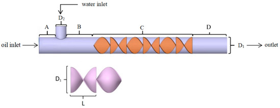
Figure 1.
Physical modeling of static mixer.

Table 1.
Structure of SK static mixer.
The physical parameters of the crude oil and sodium hypochlorite solution utilized in this study are presented in Table 2.
Table 2.
Physical properties.
The initial H2S concentration for this simulation was predominantly based on field investigation data reported by Townsend-Small et al. [29]. Their study indicated that H2S concentrations commonly reach hazardous levels (above 100 ppm) in most oil well environments. To ensure the practical relevance of the simulation results while maintaining computational efficiency, an initial H2S concentration of 100 mg/kg in crude oil was established.
The selection of NaClO solution concentration was informed by recent research conducted by Ghalwa’s group, which demonstrated that electrolysis of sodium chloride solution using Pb/PbO2 electrodes can yield NaClO solutions with effective chlorine concentrations of up to 20 g/kg [30]. Given the relatively low initial H2S concentration in our simulation system, a NaClO concentration of 10 g/kg was chosen for the reaction simulation following thorough evaluation. This concentration not only optimizes reaction efficiency but also minimizes reagent waste, ensuring sufficient reaction completion and economic viability for practical industrial applications.
In the numerical simulation setup, the inlet boundary conditions for both the crude oil and sodium hypochlorite solution were designated as velocity inlets, while the outlet boundary conditions were configured as outflow. The inlet flow rate of the crude oil was set at 1 m/s, and the volume flow ratio between the crude oil and the sodium hypochlorite solution was maintained at 20:1 throughout the simulation.
2.2. Computational Method and Assumptions
This study utilizes Fluent 14.5 software for numerical simulations, employing the Eulerian-Eulerian multiphase flow model. The realizable k-ϵ model is chosen as the turbulence model, while the Standard Wall Function (SWF) [31] is applied for boundary definition. The pressure-based SIMPLE algorithm is used to compute the flow field, and the second-order upwind scheme is employed to solve the pressure, momentum, and energy equations. In this simulation, the mixing cells and walls are treated as fixed walls.
The continuity and momentum equations [31] are as follows:
where is the volume fraction of the phase q. is the density of the qth-phase, kg/m3. is the velocity of the phase q, m/s. is the gravitational acceleration, m/s2. is the sum of all the forces on the qth-phase, N. is the pressure, Pa. is the effective viscosity, Pa·s.
where is the continuous-phase molecular viscosity, Pa·s. is the turbulent viscosity, Pa·s.
The turbulence kinetic energy equation [21] is as follows:
where is the turbulent kinetic energy generation term due to the mean velocity gradient, W/m3. is the turbulent kinetic energy generation term due to buoyancy, W/m3. is the turbulence dissipation rate. is the dissipation term of the turbulent kinetic energy, W/m3. is the Planck numbers corresponding to the turbulent kinetic energy k. is the Planck numbers corresponding to the dissipation rate . and are the empirical constants. is the user-defined source term, W/m3.
The Euler-Euler model offers interphase interaction models to simulate mass transfer and chemical reaction processes. Within this framework, users can define mass transfer rates, reaction kinetics, source terms, and other critical parameters through User Defined Functions (UDFs), facilitating a more accurate simulation of mass transfer and reaction behaviors in real-world industrial processes. The mass transfer rate equations and reaction kinetics employed in this study are derived from the research findings of Vilmain et al. [6].
The reaction equation is as follows:
The reaction kinetic equation is as follows:
where is the reaction rate, mol/(L∙s). is the reaction rate constant, = 6.75 × 10⁶ L/(s∙mol) (The reaction temperature is 293 K). is the concentration of hydrogen sulfide in crude oil, mol/L. is the concentration of sodium hypochlorite in the solvation, mol/L.
The mass transfer rate equation is as follows:
where is the solute concentration in the bulk, mol/m3. is the solute concentration in equilibrium, mol/m3. is the aqueous phase diffusion coefficient of hydrogen sulfide, = 1.75 × 10⁻⁹ m2/s (The mass transfer temperature is 293 K).
The Population Balance Model (PBM) establishes population balance equation (PBE) for droplet number density based on the microscopic dynamics of dispersed-phase droplets, including processes such as breakup, agglomeration, and growth [32]. This model has found widespread applications in chemical engineering, food processing, bioengineering, and emulsion research. The primary objective of employing the PBM in this study is to analyze the behavior of droplet breakup and agglomeration within the static mixer. In the PBM framework, the Luo model [29] is adopted for the breakup process, while a turbulent model [30] is utilized for the agglomeration process.
In Fluent 14.5, the PBE can be solved using the finite volume method. The transport equation for the number density function is as follows [33,34]:
where V is the droplet breakage volume fraction, m3. is the number density distribution function. u is the solvent velocity, m/s. represents the droplet aggregation and birth function of volume V. represents the droplet aggregation and death function of size L. represents the droplet breakage birth function of volume V. represents the droplet fragmentation death function of volume V.
The droplet breakup rate equation is as follows [35,36]:
where is the ratio of the turbulent vortex diameter to the diameter of the broken droplet. is the interfacial tension, N/m2. is the volume ratio of the crushed sub-droplet to the mother droplet. is the continuous-phase density, kg/m3.
The droplet aggregation rate equation is as follows [37,38]:
where is rate the viscous subrange. is rate the inertial subrange. is the pre-factor that considers the collision capture efficiency coefficient due to turbulence. is the shear rate. is the mean square velocity of droplet, m/s.
The computational process of the CFD-PBM coupled model is outlined as follows: First, local flow field parameters, including phase volume fractions and turbulence dissipation rates, are obtained through CFD simulations. These parameters are subsequently input into the PBM model, which incorporates droplet breakup and coalescence kinetic models to calculate the non-uniform droplet size distribution. Based on the resulting distribution, the interaction forces between the liquid phases in the CFD model and the turbulence kinetic energy are dynamically corrected. This forms a closed-loop iterative computational mechanism that enables the synergistic optimization of flow field information and particle size distribution. The specific schematic diagram of the CFD-PBM coupling model is shown in Figure 2.
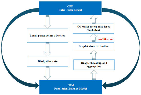
Figure 2.
Schematic diagram of the CFD-PBM coupling model.
The main assumptions underlying this study are as follows:
- The acceleration of gravity is 9.81 m/s2 in the direction of the z-axis.
- Each phase of the multiphase flow is assumed to be an incompressible fluid [39,40].
- The surfaces of the mixing elements are assumed to be smooth, and their turbulent effects arise only from fluid shear [41,42].
- In this study, the volumetric flow rate of crude oil significantly exceeds that of the aqueous phase. Therefore, crude oil is set as the continuous phase and water is set as the dispersed phase during oil-water mixing.
- Mass transfer occurs exclusively at the oil-water interface.
2.3. Characterization Methods
2.3.1. Hydrogen Sulfide Removal Efficiency
The hydrogen sulfide removal efficiency (HSRE) was utilized to assess the effectiveness of the H2S removal process. A higher HSRE value indicates a more effective process for removing hydrogen sulfide from crude oil within the static mixer.
where is the average mass fraction of H2S in the crude oil within the cross-section grid, mg/kg. imports the mass fraction of H2S in the crude oil within the inlet cross-section grid.
2.3.2. Mixing Effect
- The coefficient of variation (CoV) is used to evaluate the mixing effectiveness, representing the deviation of the crude oil volume fraction at the sampling point from the average volume fraction of crude oil across the entire cross-section. A lower CoV indicates a better mixing effect [43].where N is the number of grids in the static mixer cross-section, and, in this paper, we take N to be 2000. is the volume fraction of oil-phase components in each grid. is the average volume fraction of crude oil at the entire outlet plane.
- Mixing efficiency was further assessed using the micro-mixing time (tm, in seconds). This parameter indicates the time required to achieve homogeneous mixing of crude oil and water at a microscopic level. A lower tm value reflects a higher mixing efficiency of the static mixer [44].where represents the kinematic viscosity of the continuous phase fluid, m2/s. denotes the energy dissipation rate per unit time in the mixer (calculated by simulation software, m2/s3).
2.3.3. Droplet Dispersion Effect
To evaluate the dispersion performance of the static mixer, this study introduces the Sauter mean diameter (SMD, d32) as a quantitative indicator. The d32 is directly related to the specific surface area of the dispersed phase (the surface area per unit volume ∝ 1/d32); a larger specific surface area leads to higher rates of mass transfer, heat transfer, or reaction. Additionally, d32 also reflects the uniformity of the dispersion; a smaller value indicates a higher proportion of small droplets in the system, signifying superior dispersion performance [45].
where is the droplet diameter, mm. is the number of droplets with diameter .
2.3.4. Differential Pressure
Differential pressure refers to the pressure drop resulting from frictional resistance, turbulent dissipation, and interphase interactions as the fluid flows through the mixing equipment. A lower pressure drop is preferable, as long as the process requirements are satisfied.
where is the pressure at the inlet, kPa. is the pressure at the outlet, kPa.
2.4. Grid Irrelevance Test
In this study, Fluent Meshing was employed to construct the hexahedral mesh for the SK static mixer. The mixer parameters included 10 elements, an aspect ratio (L/D1) of 1, and a twist angle of 90°. Five mesh sizes were utilized: 1 mm, 0.1 mm, 0.01 mm, 0.001 mm, and 0.0001 mm, corresponding to grid numbers of 213,983; 246,897; 379,328; 423,896; and 513,215, respectively. The simulations were conducted under the following conditions: an H2S concentration in crude oil of 100 mg/kg, a NaClO concentration in water of 10 g/kg, an oil flow velocity of 1 m/s, and a water flow velocity of 0.1125 m/s.
The calculation results are shown in Figure 3. When the mesh size of the SK-type static mixer is set to 0.0001 mm, the HSRE values are essentially consistent with those obtained at mesh sizes of 0.001 mm (with a variation of HSRE less than 0.9%). Therefore, it can be concluded that the use of a mesh size of 0.001 mm meets the grid independence verification criteria.
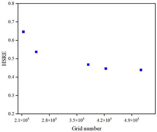
Figure 3.
The effect of the number of grids on the results.
2.5. Model Validation
Based on the hydrogen sulfide removal experimental results from crude oil reported by Shen [10], the reliability of the UDFs used in this simulation has been verified. The physical model and boundary conditions of the static mixer in the simulation are consistent with those of the aforementioned experiment: the static mixer has a length of 250 mm and a diameter of 15 mm, equipped with 7 SK-type elements. The flow rate of the aqueous solution is set at 30 mL/min, while the oil-water ratio is increased from 25:1 to 45:1 by varying the crude oil flow rate.
The simulated values of H2S content in the crude oil at the outlet of the static mixer were compared with the experimental values, as shown in Table 3. There is a discrepancy between the simulation results and the experimental results, primarily due to the mass transfer and reaction equations used in the simulation being investigated at a temperature of 293 K, while the oil temperature during the experiment was 338 K and the NaClO solution temperature was 298 K. However, the absolute difference between the simulation and experimental values is less than 4 mg/kg, and the overall trends are consistent, indicating that the numerical model is accurate, reasonable, and applicable.
Table 3.
Comparative analysis of simulation and experimental results.
A reliability check of the PBM method employed in this paper is based on the experimental results of toluene-water two-phase mixing in an SK-type static mixer, as investigated by Wang et al. [46]. The physical model of the static mixer used in the simulation is consistent with the experimental setup: the tube length is 500 mm, the inner diameter is 24 mm, 10 SK-type elements are installed, and the aspect ratio of the mixing elements is 1.5. Distilled water was set as the continuous phase, while toluene served as the dispersed phase. Simulation was conducted using the experimental conditions from groups 2, 3, 7, and 10 of the response surface experiments described by Wang et al. The simulated value of d32 at the outlet of the static mixer was compared with the experimental values, and the results are presented in Table 4. Notably, the relative errors between the simulated and experimental values are within 10%.
Table 4.
Comparative analysis of simulation and experimental results.
3. Results and Discussion
3.1. Structural Optimization of SK Static Mixer
Using a static mixer with a diameter of 15 mm, the effects of the number of elements (A), aspect ratio (B), and twist angle (C) on the hydrogen sulfide removal efficiency (HSRE) were investigated through response surface methodology. The study was conducted under the following conditions: 100 mg/kg H2S in crude oil, 10 g/kg NaClO in water, a crude oil velocity of 1 m/s, and a water velocity of 0.1125 m/s. The simulated data are presented in Table 5, Table 6 and Table 7. Table 5 details the factors and levels of the Box-Behnken experiment.
Table 5.
Factors and levels of Box-Behnken experiment.
Table 6.
Results of Box-Behnken experiment.
Table 7.
Analysis of Variance.
Figure 4 illustrates the crude oil path-lines for experiments No. 1 and 2. The geometry of the mixing elements generates shear and turbulent disturbances, which accelerate fluid flow within the channel. Increasing the number of elements enhances multi-scale fluid cutting, turbulent pulsation, and mixing uniformity, thereby disrupting the crude oil–water phase boundary. This disruption promotes the diffusion of NaClO, facilitating mass transfer and its reaction with H2S, ultimately resulting in improved hydrogen sulfide removal efficiency.
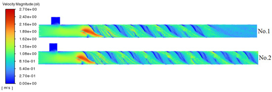
Figure 4.
Path-lines of crude oil for No. 1 and No. 2 experiments.
Figure 5 presents the path-lines for experiments No. 1 and 3. A smaller aspect ratio (which corresponds to more compact mixing units) enhances fluid cutting, folding, and redistribution within a shorter flow path. This configuration reduces residence time, induces local acceleration through narrow passages, increases turbulence and shear, disrupts liquid boundary layers, and enlarges the liquid-liquid contact area. Furthermore, it minimizes flow resistance, enabling higher flow rates for the same pressure drop. These combined effects all contribute to facilitating the hydrogen sulfide removal efficiency.
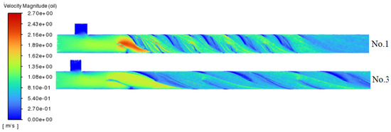
Figure 5.
Path-lines of crude oil for No. 1 and No. 3 experiments.
Figure 6 illustrates the path-lines for experiments No. 9 and 11. The mixing elements configured at 45° and 90° generate shear and turbulence by altering the flow direction. The 90° configuration leads to sharp deflections and localized high-pressure zones, while the 45° configuration induces oblique shear and facilitates kinetic energy transfer through successive splitting and reconvergence. Despite their differing mechanisms, both configurations result in a comparable increase in flow velocity, with no significant differences observed between them.
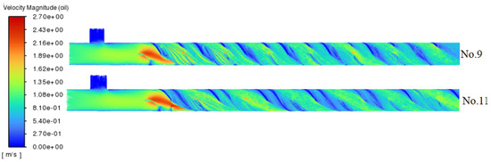
Figure 6.
Path-lines of crude oil for No. 9 and No. 11 experiments.
A second-order polynomial model was constructed to predict hydrogen sulfide removal efficiency (HSRE) based on the design matrix. The model was fitted using MATLAB 24.1 software, resulting in the following Equation (22):
In the equation, Y represents the predicted hydrogen sulfide removal efficiency (HSRE). The model indicates that the linear terms A (number of elements) and C (twist angle), as well as the quadratic term B2 (aspect ratio), have a positive effect on HSRE. Conversely, the linear term B and the interaction terms AB, AC and BC, along with the quadratic terms A2 and C2, exert a negative effect on HSRE. The analysis of variance (ANOVA) presented in Table 7 indicates a significant model (F = 22.58, p < 0.05) with a high coefficient of determination (R2 = 0.9855), confirming the reliability and predictive capability of the model.
Three-dimensional response surface analysis (Figure 7, Figure 8 and Figure 9) revealed a positive correlation between hydrogen sulfide removal efficiency (HSRE) and the number of elements, while a negative correlation was observed with the aspect ratio. The twist angle demonstrated a negligible influence (p > 0.05), and no significant interactions were found between the variables. The optimal conditions determined through stepwise regression and response surface analysis were identified as 15 elements, an aspect ratio of 1 and a twist angle of 90°. Under these optimal conditions, the simulation yielded an HSRE of 0.7202 (corresponding to an outlet H2S concentration of 27.98 mg/kg), with a model-predicted value of 0.6601, resulting in an error of 8.34%.
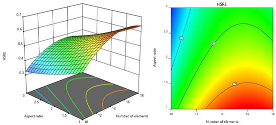
Figure 7.
Response surface diagram and contour diagram of the interaction between number of elements and aspect ratio on HSRE.
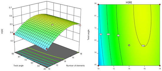
Figure 8.
Response surface diagram and contour diagram of the interaction between number of elements and twist angle on HSRE.
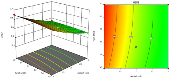
Figure 9.
Response surface diagram and contour diagram of the interaction between aspect ratio and twist angle on HSRE.
3.2. Static Mixer Performance
Simulation was employed to compare the fluid flow characteristics in the optimized static mixer with those in an isometric empty pipe, focusing on their effects on mixing, hydrogen sulfide removal efficiency (HSRE), and pressure drop (P). The inlet conditions for both systems were maintained consistent with those specified in Section 3.1.
3.2.1. Hydrogen Sulfide Removal Efficiency
The static mixer demonstrated a substantial reduction in H2S concentration, with the outlet hydrogen sulfide removal efficiency (HSRE) increasing from 0.0363 in the empty pipe to 0.7202 in the optimized static mixer (as shown in Figure 10). Figure 11 illustrates a positive correlation between the number of elements and the HSRE, which increased from 0.1815 with 3 elements to 0.7184 with 15 elements, thereby confirming the efficacy of the SK mixer in enhancing hydrogen sulfide removal efficiency.
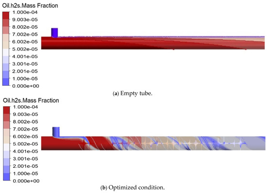
Figure 10.
Contour map of H2S mass fraction.
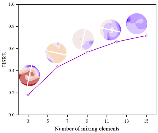
Figure 11.
Effect of the number of mixing elements on HSRE.
3.2.2. Mixing Effect
Figure 12 compares the oil volume fraction distributions in the static mixer and the empty pipe. The empty pipe exhibits smooth laminar flow with a distinct oil-water interface, while the static mixer induces alternating rotational motions that enhance radial fluid exchange and promote oil-water mixing. The mixing efficiency was quantified using the coefficient of variation (CoV) and micro-mixing time (tm). The CoV decreased from 0.8798 to 0.2143, indicating improved mixing homogeneity. Additionally, tm was reduced from 0.04593 s to 0.001 s, signifying an increase in mass exchange between fluid micro-clusters per unit time and enhanced mixing efficiency. The data presented in Figure 13 show that by increasing the number of elements from 3 to 15, the CoV was reduced by a factor of 3.21, and tm decreased by a factor of 45.51, demonstrating the superior mixing efficiency of the static mixer.
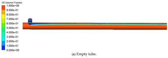
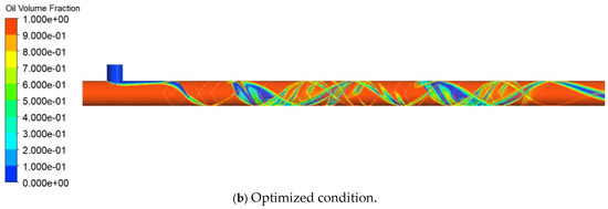
Figure 12.
Cloud map of oil-water two-phase distribution.
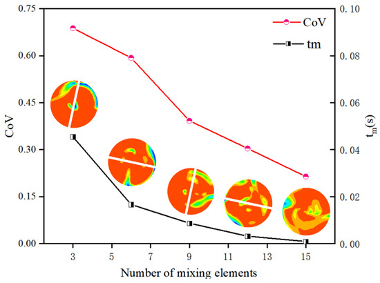
Figure 13.
Effect of number of mixing elements on CoV and tm.
In summary, the static mixer significantly enhances oil-water contact efficiency by increasing turbulent mixing effects. This improvement accelerates both the mass transfer and reaction rates of H2S, ultimately leading to highly efficient hydrogen sulfide removal.
3.2.3. Differential Pressure
The radial pressure drop cloud diagrams for the static mixer and empty pipe are illustrated in Figure 14. The radial pressure drop increased from 2.796 kPa in the empty pipe to 19.28 kPa in the static mixer. While mixing efficiency improved with the addition of more elements, the pressure drop also increased proportionally. This rise in pressure drop indicates enhanced turbulent intensity, characterized by stronger vortices and shear forces during fluid passage through the mixer. Such turbulence reduces the thickness of the oil-water mass transfer boundary layer, thereby accelerating the mass transfer and reaction rates of H2S, ultimately leading to improved hydrogen sulfide removal efficiency. Consequently, it can be concluded that reducing the number of mixing elements should be prioritized, provided that the process requirements are satisfactorily met.
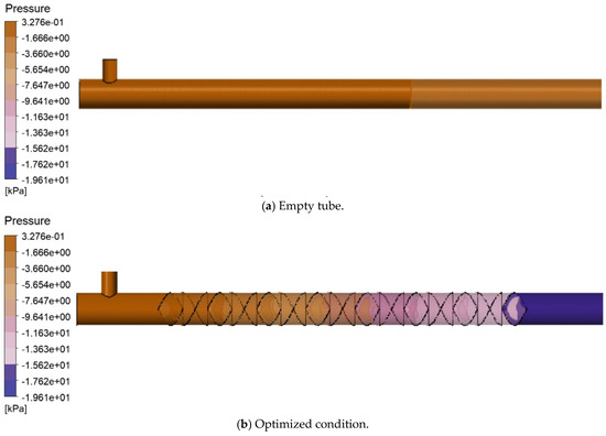
Figure 14.
Cloud map of radial pressure drop.
3.3. Water Inlet Diameter
The maximum size of water droplets is influenced by the diameter of the water inlet diameter. To systematically analyze the effect of maximum droplet size, the impact on droplet size in a static mixer was studied by varying the diameter of the water inlet diameter. Droplet dispersion was assessed using the Sauter Mean Diameter (d32), where a smaller d32 indicates more effective fluid breakup.
Figure 15 illustrates that the water inlet diameter ranged from 0.1 mm to 10 mm. The d32 does not decrease significantly after 12 mixing elements. Initially, as the number of elements increases, the d32 reduces due to the high shear forces that break up large droplets. However, as more elements are added, the aggregation of small droplets becomes more pronounced. When the number of mixing elements exceeds 12, the processes of droplet fragmentation and aggregation reach a dynamic equilibrium, causing the d32 to stabilize. Consequently, further increases in the number of elements have a diminishing effect on the d32. Notably, the d32 at the static mixer outlet is slightly higher than that observed with 15 mixing elements. After exiting the static mixer, the droplets primarily coalesce, a phenomenon attributed to the reduced shear forces and turbulent dissipation, which increase droplet collision frequency and promote aggregation. Additionally, surface tension drives the coalescence of smaller droplets to minimize interfacial energy. It was also observed that for configurations with 3, 6, 9, and 12 mixing elements, when the water inlet diameter exceeded 1 mm, its influence on the final d32 was significantly reduced. During the early mixing stage (e.g., within the first 12 elements), although large droplets (>1 mm) were not fully fragmented, their low proportion meant that the d32 was mainly determined by smaller droplets. As the number of mixing elements increased beyond 12, droplet fragmentation approached its limit, leading to a diminished effect of the initial maximum droplet size on the d32.
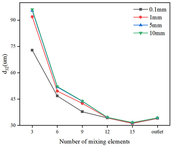
Figure 15.
Effect of number of mixing elements on d32.
Figure 16 presents droplet size distributions (DSD) for various water inlet diameters (0.1 mm, 1 mm, 5 mm, and 10 mm). The distributions reveal a dominance of droplets within the size range of 0.001 mm to 0.1 mm. As the number of mixing elements increases, the DSDs exhibit narrower normal distributions and a higher proportion of smaller droplets. This trend reflects the continuous shear-induced fragmentation process and the dynamic equilibrium established between fragmentation and aggregation within the static mixer.
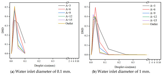
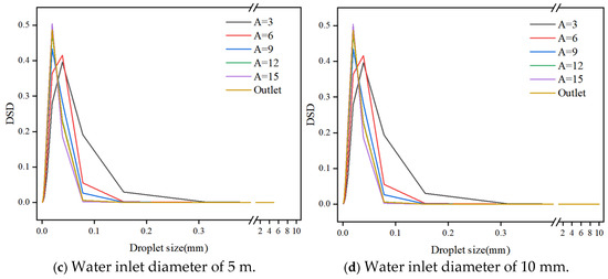
Figure 16.
Droplet size distribution for different water inlet diameter.
The comprehensive results of the above analysis demonstrate that the static mixer significantly increases the oil-water contact interface area by facilitating the uniform dispersion of droplets. This enhanced dispersion, in turn, improves the mass transfer and reaction processes of H2S, ultimately leading to a substantial increase in removal efficiency.
4. Conclusions
This study demonstrates the effectiveness of SK static mixers for H2S removal from crude oil by employing a combined CFD-PBM approach. Structural optimization using response surface methodology revealed that increasing the number of elements to 15 and reducing the aspect ratio to 1:1 maximized turbulent shear and contact between reactant interfaces, achieving an H2S removal efficiency of 72.02%. This represents a significant improvement over conventional empty tubes, which exhibited an efficiency of only 3.63%. The optimized geometry induced multi-scale fluid folding and radial momentum exchange, resulting in a reduction of micro-mixing time (tm) to 0.001 s and a 75.6% decrease in phase separation, as indicated by a coefficient of variation (CoV) of 0.21. While the pressure drop increased linearly with the number of elements (recording 19.28 kPa compared to 2.80 kPa for the empty tube), the trade-off between energy consumption and process efficiency favors the use of static mixers for fast oxidation reactions, such as those occurring in NaClO-H2S systems. Furthermore, droplet dispersion analysis revealed that the Sauter Mean Diameter (d32) stabilized after 12 mixing elements, with 95% of the droplets measuring below 0.1 mm. This small droplet size provides sufficient interfacial area to facilitate effective mass transfer.
The numerical simulations in this study incorporate necessary simplifying assumptions; however, actual industrial flow conditions are inherently more complex. This discrepancy represents a primary limitation of our current approach. Future studies should concentrate on developing correction models through systematic experimental validation to enhance the industrial applicability of the optimized mixer design.
Supplementary Materials
The following supporting information can be downloaded at: https://www.mdpi.com/article/10.3390/pr13051515/s1, Figure S1: Influence of oil-water ratio on mixing effect and HSRE; Figure S2: Effect of oil-water ratio on P; Figure S3: Effect of H2S concentration at the inlet on HSRE; Figure S4: Effect of crude oil density on HSRE, CoV, tm and P; Figure S5: Effect of crude oil viscosity on HSRE, CoV, tm and P; Figure S6: Effect of NaClO concentration on HSRE.
Author Contributions
M.G.: simulation calculations, writing—original draft; J.L.: simulation calculations tests; Y.C.: methodology; Z.H.: supervision; H.W.: data curation; P.Y.: formal analysis; X.X.: validation; J.Y.: writing—review and editing. All authors have read and agreed to the published version of the manuscript.
Funding
This research was funded by National Natural Science Foundation of China (22178113).
Data Availability Statement
Data are contained within the article and Supplementary Materials.
Conflicts of Interest
Author Jiacheng Liu, Ying Chen and Hongfu Wang were employed by the company Santacc Energy Co., Ltd. The remaining authors declare that the research was conducted in the absence of any commercial or financial relationships that could be construed as a potential conflict of interest.
References
- Sun, H.; Zhong, L.; Zhu, Y.; Zhu, J.; Li, Z.; Zhang, Z.; Zhou, Y. Assessing sulfate-reducing bacteria influence on oilfield safety: Hydrogen sulfide emission and pipeline corrosion failure. Eng. Fail. Anal. 2024, 164, 108646. [Google Scholar] [CrossRef]
- Marriott, R.A.; Pirzadeh, P.; Marrugo-Hernandez, J.J.; Raval, S. Hydrogen sulfide formation in oil and gas. Can. J. Chem. 2016, 94, 406–413. [Google Scholar] [CrossRef]
- Guzenkova, A.S.; Artamonova, I.V.; Guzenkov, S.A.; Ivanov, S.S. Steel Corrosion in Hydrogen Sulfide Containing Oil Field Model Media. Metallurgist 2021, 65, 517–521. [Google Scholar] [CrossRef]
- Sun, H.; Zhong, L.; Zhu, Y.; Zhu, J.; Zhou, Y. Risk prediction for hydrogen sulfide emission based on sulfate-reducing bacteria in the water flooding oilfield. Phys. Fluids 2024, 36, 057119. [Google Scholar] [CrossRef]
- Almasvandi, M.H.; Rahimi, M.; Tagheie, Y. Microfluidic cold stripping of H2S from crude oil in low temperature and natural gas consumption. J. Nat. Gas Sci. Eng. 2016, 34, 499–508. [Google Scholar] [CrossRef]
- Vilmain, J.-B.; Courousse, V.; Biard, P.-F.; Azizi, M.; Couvert, A. Kinetic study of hydrogen sulfide absorption in aqueous chlorine solution. Chem. Eng. Res. Des. 2014, 92, 191–204. [Google Scholar] [CrossRef]
- Busca, G.; Pistarino, C. Technologies for the abatement of sulphide compounds from gaseous streams: A comparative overview. J. Loss Prev. Process Ind. 2003, 16, 363–371. [Google Scholar] [CrossRef]
- Wang, Y.; Zhang, H.; Zhang, X.; Lu, F.; Wang, W.; Zhang, Y.; Nie, Q.; He, P. Dual roles of odor cleaners and pollutant producers for chemical scrubbing and biological treatment: Evidence in a food waste anaerobic digestion plant. Chem. Eng. J. 2024, 496, 153898. [Google Scholar] [CrossRef]
- Taylor, R.A.; Penney, W.R.; Vo, H.X. Scale-up Methods for Fast Competitive Chemical Reactions in Pipeline Mixers. Ind. Eng. Chem. Res. 2005, 44, 6095–6102. [Google Scholar] [CrossRef]
- Shen, Y. Study on Technology of Removing Hydrogen Sulfide from Crude Oil. Master’s Thesis, China University of Petroleum (East China) Shandong, Qingdao, China, 2010. [Google Scholar]
- Khinast, J.G.; Bauer, A.; Bolz, D.; Panarello, A. Mass-transfer enhancement by static mixers in a wall-coated catalytic reactor. Chem. Eng. Sci. 2003, 58, 1063–1070. [Google Scholar] [CrossRef]
- Madhuranthakam, C.M.R.; Pan, Q.; Rempel, G.L. Continuous process for production of hydrogenated nitrile butadiene rubber using a Kenics® KMX static mixer reactor. AlChE J. 2009, 55, 2934–2944. [Google Scholar] [CrossRef]
- Li, D.; Xiong, K.; Yang, Z.; Liu, C.; Feng, X.; Lu, X. Process intensification of heterogeneous photocatalysis with static mixer: Enhanced mass transfer of reactive species. Catal. Today 2011, 175, 322–327. [Google Scholar] [CrossRef]
- Al Taweel, A.M.; Azizi, F.; Sirijeerachai, G. Static mixers: Effective means for intensifying mass transfer limited reactions. Chem. Eng. Process. Process Intensif. 2013, 72, 51–62. [Google Scholar] [CrossRef]
- Ren, X.; Mei, Y.; Feng, M.; Li, B.; Lyu, W.; Wen, Y.; Wang, C.; He, D. Process intensification of removing arsenic from industrial phosphoric acid by Keltics static mixer. CIESC J. 2018, 69, 218–225. [Google Scholar]
- Biard, P.-F.; Dang, T.T.; Bocanegra, J.; Couvert, A. Intensification of the O3/H2O2 advanced oxidation process using a continuous tubular reactor filled with static mixers: Proof of concept. Chem. Eng. J. 2018, 344, 574–582. [Google Scholar] [CrossRef]
- Gong, H.; Gao, L.; Nie, K.; Wang, M.; Tan, T. A new reactor for enzymatic synthesis of biodiesel from waste cooking oil: A static-mixed reactor pilot study. Renew. Energy 2020, 154, 270–277. [Google Scholar] [CrossRef]
- Chetpattananondh, P.; Tabtimmuang, A.; Prasertsit, K. Enhanced Glycerolysis of Fatty Acid Methyl Ester by Static Mixer Reactor. ACS Omega 2024, 9, 39703–39714. [Google Scholar] [CrossRef]
- Liu, Y.; Liu, M.; Huang, Z.; Wang, H.; Yuan, P.; Xu, X.; Yang, J. Numerical simulation of the mixing and salt washing effects of a static mixer in an electric desalination process. Processes 2024, 12, 883. [Google Scholar] [CrossRef]
- Lupo, M.; Sofia, D.; Barletta, D.; Poletto, M. Calibration of DEM Simulation of Cohesive Particles. Chem. Eng. Tran. 2019, 74, 379–384. [Google Scholar]
- Haddadi, M.M.; Hosseini, S.H.; Rashtchian, D.; Ahmadi, G. CFD modeling of immiscible liquids turbulent dispersion in Kenics static mixers: Focusing on droplet behavior. Chin. J. Chem. Eng. 2020, 28, 348–361. [Google Scholar] [CrossRef]
- Deng, J.; Wu, J.; Han, L.; Zhou, Y. CFD-PBM coupled modeling of liquid-liquid interphase mass transfer behaviors inside the Kenics static mixer. Powder Technol. 2024, 445, 120119. [Google Scholar] [CrossRef]
- Cao, Q.; Zhou, J.; Qian, Y.; Yang, S. Three-Dimensional Model on Liquid–Liquid Mass Transfer of the Kenics Static Mixer: Considering Dynamic Droplet Size Distribution. Ind. Eng. Chem. Res. 2023, 62, 10507–10522. [Google Scholar] [CrossRef]
- Meng, H.; Meng, T.; Yu, Y.; Wang, Z.; Wu, J. Experimental and numerical investigation of turbulent flow and heat transfer characteristics in the Komax static mixer. Int. J. Heat Mass Transf. 2022, 194, 123006. [Google Scholar] [CrossRef]
- Albertazzi, J.; Florit, F.; Busini, V.; Rota, R. A novel Static Mixer for photochemical reactions. Chem. Eng. Process. Process Intensif. 2022, 182, 109201. [Google Scholar] [CrossRef]
- Moon, D.H.; Park, S.S.; Kang, S.-P.; Lee, W.; Park, K.T.; Chun, D.H.; Rhim, G.B.; Hwang, S.-M.; Youn, M.H.; Jeong, S.K. Determination of kinetic factors of CO2 mineralization reaction for reducing CO2 emissions in cement industry and verification using CFD modeling. Chem. Eng. J. 2021, 420, 129420. [Google Scholar] [CrossRef]
- Xie, Y.; Liu, J.; Li, J.; Yang, B. Study on Ozone Oxidation Regeneration of Ce3+ Enhanced by a Static Mixer. J. Chem. Eng. Chin. Univ. 2017, 31, 1318–1326. [Google Scholar]
- Santana, H.S.; Tortola, D.S.; Silva, J.L.; Taranto, O.P. Biodiesel synthesis in micromixer with static elements. Energy Convers. Manag. 2017, 141, 28–39. [Google Scholar] [CrossRef]
- Townsend-Small, A.; Edgar, A.; Fernandez, J.M.; Jackson, A.; Currit, N. High rates of hydrogen sulfide emissions measured from marginal oil wells near Austin and San Antonio, Texas. Environ. Res. Commun. 2024, 6, 091007. [Google Scholar] [CrossRef]
- Ghalwa, N.A.; Tamos, H.; ElAskalni, M.; El Agha, A.R. Generation of sodium hypochlorite (NaOCl) from sodium chloride solution using C/PbO2 and Pb/PbO2 electrodes. Int. J. Min. Met. Mater. 2012, 19, 561–566. [Google Scholar] [CrossRef]
- Li, B.; Huang, C.; Liu, L.Y.; Yao, L.; Ning, B.; Yang, L. Separation efficiency prediction of non-Newtonian oil-water swirl-vane separators in offshore platform based on GA-BP neural network. Ocean Eng. 2024, 296, 116984. [Google Scholar] [CrossRef]
- Lei, J.; Zhang, J. Numerical simulation of aerated flow in tunnel based on CFD-PBM coupled model. Ocean. Eng. 2024, 313, 119407. [Google Scholar] [CrossRef]
- Gu, D.; Wen, L.; Xu, H.; Ye, M. Study on hydrodynamics characteristics in a gas-liquid stirred tank with a self-similarity impeller based on CFD-PBM coupled model. J. Taiwan Inst. Chem. Eng. 2023, 143, 104688. [Google Scholar] [CrossRef]
- Meng, H.; Wang, J.; Yu, Y.; Wang, Z.; Wu, J. CFD-PBM Numerical Study on Liquid-Liquid Dispersion in the Q-Type Static Mixer. Ind. Eng. Chem. Res. 2021, 60, 18121–18135. [Google Scholar] [CrossRef]
- Luo, H.; Svendsen, H.F. Theoretical model for drop and bubble breakup in turbulent dispersions. AlChE J. 2004, 42, 1225–1233. [Google Scholar] [CrossRef]
- Tan, G.; Qian, K.; Jiang, S.; Wang, J.; Wang, J. CFD-PBM Investigation on Droplet Size Distribution in a Liquid-Liquid Stirred Tank: Effect of Impeller Type. Ind. Eng. Chem. Res. 2023, 62, 4109–4121. [Google Scholar] [CrossRef]
- Abrahamson, J. Collision Rates of Small Particles In a VigorouslyI Turbulent Fluid. Chem. Eng. Sci. 1975, 30, 1371–1379. [Google Scholar] [CrossRef]
- Saffman, P.G.; Turner, J.S. On the collision of drops in turbulent clouds. J. Fluid Mech. 2006, 1, 16–30. [Google Scholar] [CrossRef]
- Bouras, H.; Haroun, Y.; Philippe, R.; Augier, F.; Fongarland, P. CFD modeling of mass transfer in Gas-Liquid-Solid catalytic reactors. Chem. Eng. Sci. 2021, 233, 116378. [Google Scholar] [CrossRef]
- Deising, D.; Marschall, H.; Bothe, D. A unified single-field model framework for Volume-Of-Fluid simulations of interfacial species transfer applied to bubbly flows. Chem. Eng. Sci. 2016, 139, 173–195. [Google Scholar] [CrossRef]
- Haroun, Y.; Legendre, D.; Raynal, L. Volume of fluid method for interfacial reactive mass transfer: Application to stable liquid film. Chem. Eng. Sci. 2010, 65, 2896–2909. [Google Scholar] [CrossRef]
- Woo, M.; Tischer, S.; Deutschmann, O.; Wörner, M. A step toward the numerical simulation of catalytic hydrogenation of nitrobenzene in Taylor flow at practical conditions. Chem. Eng. Sci. 2021, 230, 116132. [Google Scholar] [CrossRef]
- Li, H.; Yu, X.; Song, Y.; Li, Q.; Lu, S. Experimental and numerical investigation on optimization of foaming performance of the kenics static mixer in compressed air foam system. Eng. Appl. Comput. Fluid Mech. 2023, 17, 2183260. [Google Scholar] [CrossRef]
- Fournier, M.-C.; Falk, L.; Villermaux, J. A new parallel competing reaction system for assessing micromixing effciency-determination of micromixing time by a simple model. Chem. Eng. Sci. 1996, 51, 5187–5192. [Google Scholar] [CrossRef]
- Xie, R.; Li, J.; Jin, Y.; Zou, D.; Chen, M. Simulation of drop breakage in liquid–liquid system by coupling of CFD and PBM: Comparison of breakage kernels and effects of agitator configurations. Chin. J. Chem. Eng. 2019, 27, 1001–1014. [Google Scholar] [CrossRef]
- Wang, X.; Guo, W.; Wu, J. Experimental and numerical study on liquid liquiddispersion in static mixer. CIESC J. 2012, 63, 767–774. [Google Scholar]
Disclaimer/Publisher’s Note: The statements, opinions and data contained in all publications are solely those of the individual author(s) and contributor(s) and not of MDPI and/or the editor(s). MDPI and/or the editor(s) disclaim responsibility for any injury to people or property resulting from any ideas, methods, instructions or products referred to in the content. |
© 2025 by the authors. Licensee MDPI, Basel, Switzerland. This article is an open access article distributed under the terms and conditions of the Creative Commons Attribution (CC BY) license (https://creativecommons.org/licenses/by/4.0/).