Analysis of Stress Perturbation Patterns in Oil and Gas Reservoirs Induced by Faults

Abstract

The distribution of in situ stress fields in reservoirs is critical for the accurate exploration and efficient exploitation of hydrocarbon resources, especially in deep, fault-developed strata where tectonic activities significantly complicate stress field patterns. To clarify the perturbation effects of faults on in situ stress fields in deep reservoirs, this study combines dynamic–static parameter conversion models derived from laboratory experiments (acoustic emission Kaiser effect and triaxial compression tests) with a coupled “continuous matrix–discontinuous fault” numerical framework implemented in FLAC^3D6.0. Focusing on the BKQ Formation reservoir in the MH area, China, we developed a multivariate regression-based inversion model integrating gravitational and bidirectional tectonic stress fields, validated against field measurements with errors of −2.96% to 9.07%. The key findings of this study include the following: (1) fault slip induces stress reductions up to 22.3 MPa near fault zones, with perturbation ranges quantified via exponential decay functions (184.91–317.74 m); (2) the “continuous matrix–discontinuous fault” coupling method resolves limitations of traditional continuum models by simulating fault slip through interface contact elements; and (3) stress redistribution exhibits NW-SE gradients, aligning with regional tectonic compression. These results provide quantitative guidelines for optimizing hydrocarbon development boundaries and hydraulic fracturing designs in faulted reservoirs.

1. Introduction

The magnitude and distribution patterns of in situ stress in reservoirs are fundamental parameters for petroleum exploration and development. The accurate characterization of in situ stress fields in deep reservoirs plays a pivotal role in hydrocarbon reservoir exploitation [1,2]. Deep hydrocarbon reservoirs, subjected to multi-stage mineralization during hydrocarbon accumulation, frequently develop discontinuous geological structures such as faults. These discontinuities alter rock mass integrity, induce stress redistribution, and accumulate damage, thereby significantly complicating in situ stress prediction [3]. Fault-induced stress field perturbations are a complex phenomenon influenced by multiple factors, including fault geometry, mechanical properties, and regional stress conditions. Clarifying fault-induced stress perturbation is crucial for seismic hazard assessment, hydrocarbon exploration, and reservoir management.

Field-measured in situ stress data demonstrate that fault activities profoundly impact rock mass continuity and structural integrity, consequently modifying stress distribution patterns [4,5,6]. Previous studies have extensively investigated fault effects on stress fields through analytical solutions, numerical simulations, and field observations [7,8,9,10,11,12,13,14,15,16,17]. Previous studies have employed stratigraphic modeling techniques utilizing seismic data to construct reservoir and fault grid systems [18]. However, analytical methods are constrained by idealized assumptions, failing to capture accurately complex fault geometries.

The calculation model for in situ stress determination is highly dependent on the accuracy of rock mechanical parameter acquisition [19]. The vertical heterogeneity of lithological properties in deep hydrocarbon reservoirs, coupled with inherent discrepancies between dynamic and static parameter correlations, imposes additional constraints on the precision of in situ stress modeling. Researchers have implemented integrated methodologies combining laboratory-measured static rock mechanical properties with logging-derived dynamic parameters to establish dynamic–static conversion relationships for rock mechanical characterization [20]. To address modeling challenges in complex formations, researchers have adopted multi-platform collaborative approaches. Previous studies [21,22] implemented integrated modeling using Petrel and ANSYS to analyze deep reservoir stress fields through finite element methods. Multi-platform collaborative modeling effectively characterizes three-dimensional stratigraphic distributions, substantially enhancing model accuracy when based on stratigraphic frameworks. While mainstream finite element methods are widely used for stress field analysis, conventional approaches that rely on parameter weakening techniques [23] inadequately simulate discontinuous fault slip behaviors. Such limitations leads to discrepancies between simulated and actual stress magnitudes in the vicinity of faults. The finite difference-based FLAC^3D6.0 software demonstrates effectiveness in simulating regional geostress fields and capturing macroscopic stress distribution patterns [24,25]. Nevertheless, computational accuracy remains constrained by the mechanical limitations of rigid fault grid representations, leading to discernible discrepancies between simulated and in situ stress values.

To resolve these limitations, this study conducted the follows: (1) It establishes a dynamic–static parameter conversion model through the acoustic emission Kaiser effect and well-logging data integration, improving the vertical continuity of rock mechanics parameters. (2) Its proposes a “continuous matrix–discontinuous fault” coupling modeling method, dynamic–static parameter conversion (using acoustic emission and triaxial tests), to improve the vertical continuity of rock properties and assesses interface contact elements in FLAC^3D6.0 to explicitly simulate fault slip, overcoming the limitations of the traditional parameter-weakening FEM, combining physical experiments with numerical inversion to overcome traditional continuum simulation constraints. (3) It quantitatively characterizes fault disturbance ranges using exponential functions, providing scientific foundations for development boundary optimization.

2. Methodology

The accuracy of in situ stress calculation models is fundamentally dependent on the precision of rock mechanics parameters, making the acquisition of reliable mechanical properties of reservoir rocks a critical prerequisite for effective in situ stress field characterization [26]. Currently, the primary methods for obtaining reservoir rock mechanics parameters include laboratory-based rock mechanics testing and well logging interpretation [27]. Among these, rock wave velocity serves as a direct and widely used indicator of mechanical properties, enabling the calculation of key dynamic parameters such as elastic modulus and Poisson’s ratio. Conventional well logging techniques typically measure only compressional waves (P-waves) and often lack shear wave (S-wave) data, which are essential for comprehensive mechanical property analysis. In contrast, full-waveform logging provides detailed S-wave measurements, offering a more complete dataset for dynamic parameter estimation. However, the high operational costs associated with full-waveform logging limit its application primarily to exploratory wells during the early stages of reservoir development [28]. For reservoirs with only conventional well logging data, it becomes essential to establish reliable P-wave to S-wave velocity conversion relationships through targeted velocity testing. This approach enables the derivation of dynamic rock mechanics parameters, which are crucial for comprehensive reservoir analysis and stress field modeling.

All core samples analyzed in this study were obtained from the BKQ T₁b Formation reservoir in the MH area, a region characterized by complex geological conditions and significant hydrocarbon potential. To ensure the reliability and representativeness of the data, a total of 39 core samples were systematically collected from 7 vertical coring wells within the target reservoir. A structured and rigorous sampling protocol was implemented to guarantee a comprehensive coverage of the reservoir’s petrophysical characteristics, including variations in lithology, porosity, and mechanical properties. Among these samples, 32 core specimens were subjected to triaxial compression tests and acoustic emission measurements. These samples were carefully selected from varying depths and stratigraphic positions to capture the mechanical heterogeneity within the reservoir, ensuring that the results reflect the full range of geological and mechanical conditions. The coring orientation and sampling strategy are illustrated in Figure 1, providing a visual representation of the spatial distribution and sampling methodology employed in this study. This systematic approach ensures the reliability of subsequent analyses and interpretations.

Core processing strictly adhered to standards specified by the International Society for Rock Mechanics (ISRM) and the National Standard of the People’s Republic of China (GB/T 50266-2013 [29]) (Chinese National Standard for Engineering Rock Test Methods). Specimens were machined into standard cylindrical dimensions of φ25 mm × 50 mm.

2.1. Wave Velocity Testing

Laboratory acoustic wave velocity testing employed the ultrasonic method using a CTS-8077PR acoustic transmitter (Shantou Ultrasonic Electronics Co., Ltd., Shantou, China) and DS2302A oscilloscope (RIGOL Technologies Inc., Beijing, China).

Ultrasonic waves generated by the transmitter propagated through rock samples and were captured by the receiver. P-wave and S-wave velocities were calculated using Equations (1) and (2):

$$V_p={\displaystyle \frac{L}{{\mathrm{t}}_p-{\mathrm{t}}_0}}$$

(1)

$$V_s={\displaystyle \frac{L}{{\mathrm{t}}_s-{\mathrm{t}}_0}}$$

(2)

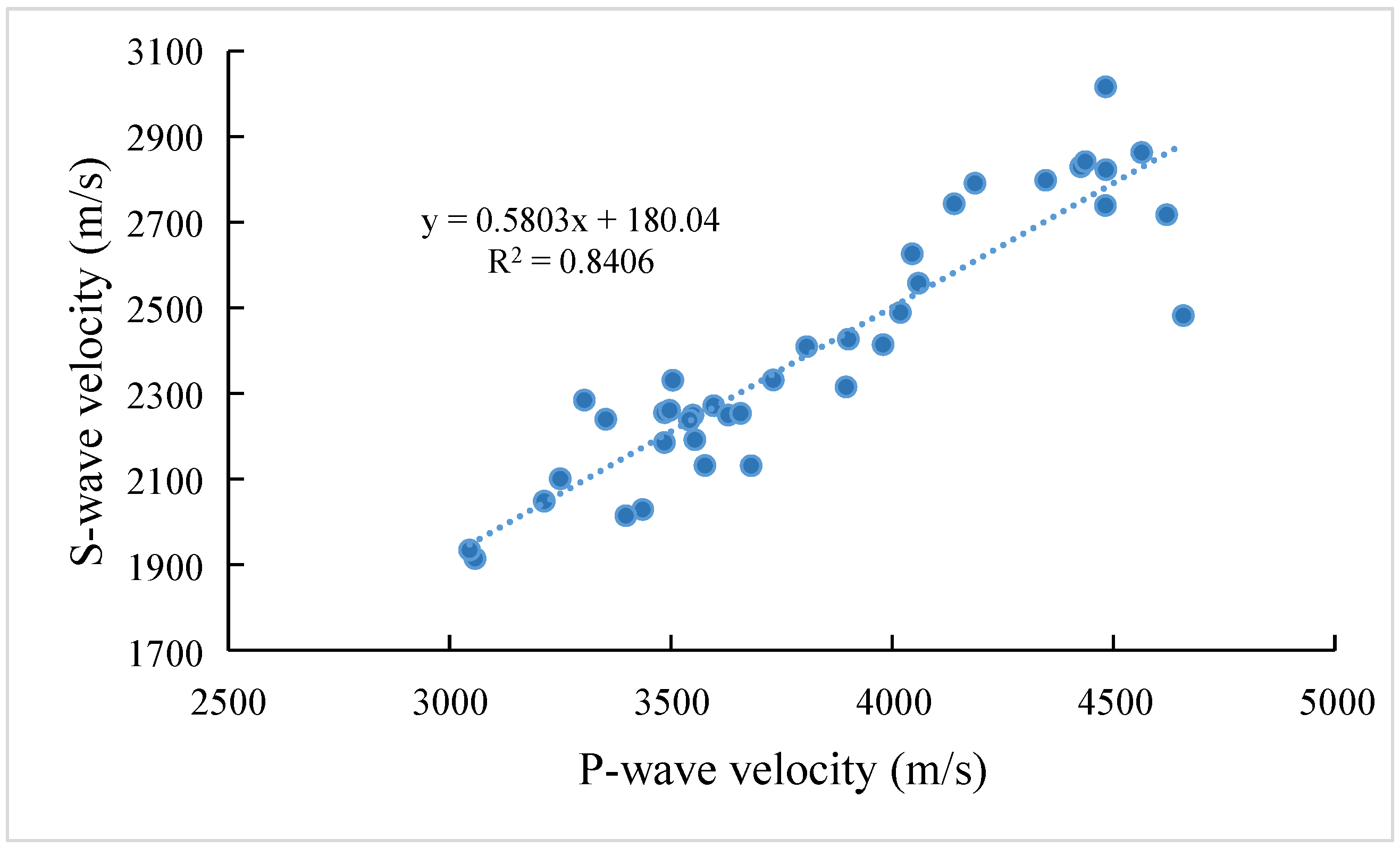
The testing results for 39 core samples yielded P-wave velocities of 3045.04–4657.83 m/s (average 3822.49 m/s) and S-wave velocities of 1914.50–3016.57 m/s (average 2398.33 m/s), with a P/S-wave velocity ratio of 1.6, indicating favorable sample integrity.

The empirical relationship V_s = 0.5803V_p + 180.04 was established for the BKQ Formation, enabling S-wave data reconstruction in conventional well logs.

While the V_p-V_s relationship exhibits minor curvature at velocity extremes (Figure 2), a linear empirical model was retained based on Castagna’s mudrock equation and Poisson’s ratio stability considerations. The moderate R² (0.8406) likely reflects sampling limitations across lithological subfacies, a constraint to be addressed in future studies through expanded core sampling and lithology-stratified modeling.

2.2. Static Rock Mechanics Parameter Testing

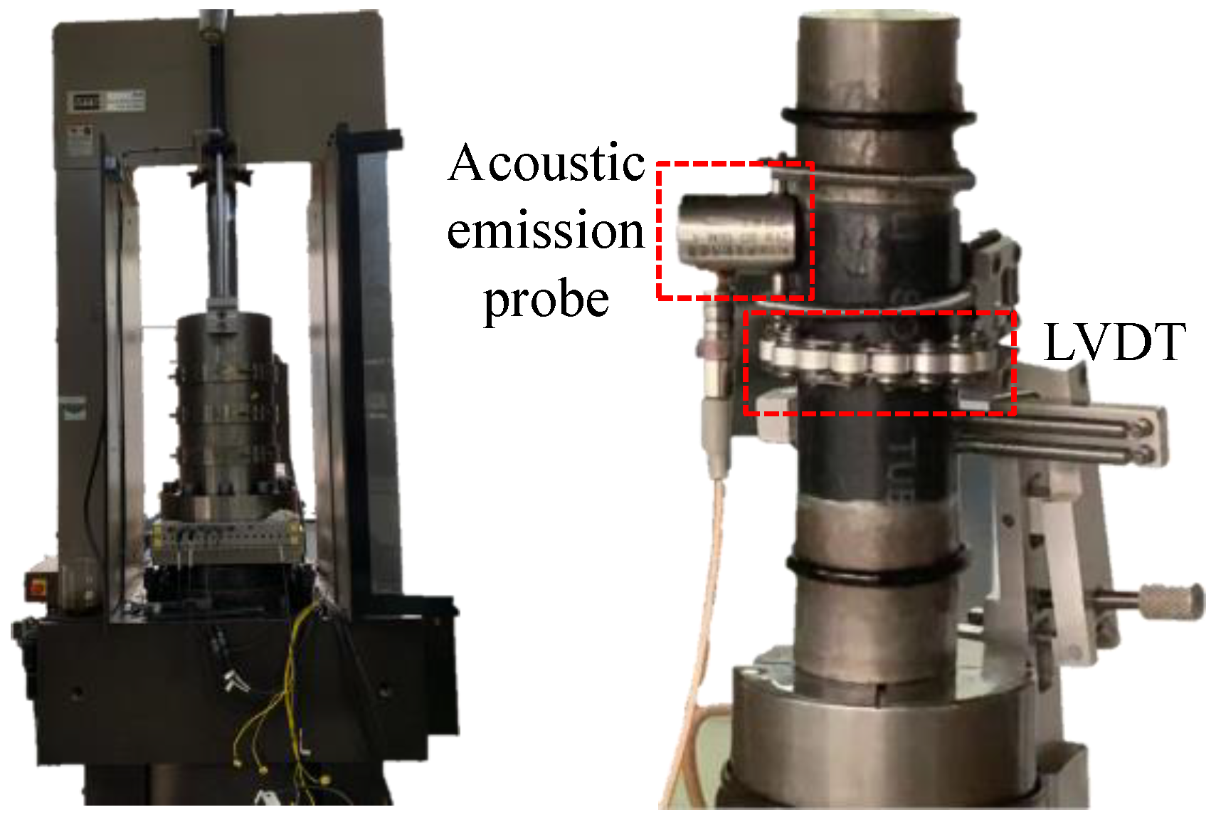
The triaxial compression test is an experimental method used to evaluate the strength and deformation characteristics of rocks under a three-dimensional stress state. The test was conducted using the MTS815.04 rock mechanics testing system (Figure 3) manufactured by MTS Corporation in the Eden Prairie, MN, United States. To determine the mechanical parameters of the rock under in situ stress conditions, particularly for the Baikouquan Formation core reservoir, it is necessary to estimate the range of confining pressure based on the effective stress formula.

Triaxial compression tests were conducted using an MTS815.04 rock mechanics system (MTS Systems Corp., Eden Prairie, MN, USA). The confinement pressure range (60–65 MPa) was determined through effective stress theory:

$${\sigma }_{\mathrm{eff}}^B=\sigma -\alpha \mathrm{p}$$

(3)

where pore pressure P_p = 70 MPa and Biot coefficient α = 0.6. The axial loading rate was 0.001 mm/s (displacement control), with confining pressure applied at 0.2 MPa/s.

The prepared specimen and the indenter were aligned and jointly inserted into a heat-shrink tube to ensure precise positioning and stability during the experiment. The LVDT (Linear Variable Differential Transformer) strain gauge and acoustic emission probe were mounted and positioned on the loading platform, with their alignment and functionality verified to ensure accurate data collection. The axial preload was applied until contact with the specimen was established, as confirmed by the pressure sensor displaying clear and consistent pressure data. Next, a high-pressure reaction vessel was lowered and securely fastened to the experimental setup. The confining pressure was incrementally increased to the preset value at the designated loading rate, ensuring controlled and consistent pressure application.

Following the establishment of the confining pressure, the axial load was applied to the specimen using the axial press, strictly adhering to the predefined loading protocol. The loading process continued until specimen failure occurred, at which point the experiment was terminated to prevent further damage. Throughout the experiment, the LVDT sensor recorded the specimen deformation, while the axial pressure sensor monitored the applied axial load. The data collected from these sensors were used to plot the stress–strain relationship curve, providing critical insights into the mechanical behavior and failure characteristics of the specimen under the applied stress conditions. Elastic modulus (E) and Poisson’s ratio (μ) were calculated at 50% peak strength:

$$E_{50}={\displaystyle \frac{{({\sigma }_1-{\sigma }_3)}_{50}}{{\epsilon }_{50}}}$$

(4)

$${\mu }_{50}={\displaystyle \frac{{\epsilon }_{\mathrm{d}50}}{{\epsilon }_{\mathrm{h}50}}}$$

(5)

Overall, 32 valid tests revealed strong heterogeneity: compressive strength: 148.08–328.55 MPa, E: 15.97–36.10 GPa, and μ: 0.16–0.25. Dynamic–static parameter conversion models were established:

$$E_s=0.1556E_d+20.008$$

(6)

$${\mu }_s=0.5494{\mu }_d+0.0282$$

(7)

2.3. Acoustic Emission Stress Test

During the compression test, as the applied stress increases, the rock begins to generate acoustic emissions (AEs), the intensity and frequency of which vary with the stress. When the applied stress reaches the maximum stress historically experienced by the rock, AE activity shows a significant increase or re-activation. This point is known as the Kaiser effect point, and the corresponding in situ stress magnitude represents the historical maximum stress, also referred to as the pre-existing stress. In compressional tectonic regions, the reservoir rock mass is under a compressive state, and the tectonic stress gradually increases with ongoing compressional movements. Therefore, in such regions, the pre-existing stress measured by the Kaiser effect reflects the in situ stress state of the reservoir.

By applying a vertical load to the specimen and using an AE probe to capture the AE signals during loading, the relationship between AE activity and axial stress can be obtained. Typically, AE-based in situ stress testing involves applying unconfined axial stress loading, i.e., uniaxial compression. However, for deep core samples, uniaxial compression may lead to specimen failure before reaching the Kaiser point. In such cases, the AE signals collected are generated by the direct fracturing of the specimen rather than corresponding to the Kaiser effect and thus cannot be used to determine the pre-existing stress of the core sample in its formation. To address this issue, this study employs axial stress loading under confining pressure, i.e., triaxial compression, for Kaiser effect-based in situ stress testing. This method simulates the formation environment of the core sample, yielding more accurate in situ stress measurement results.

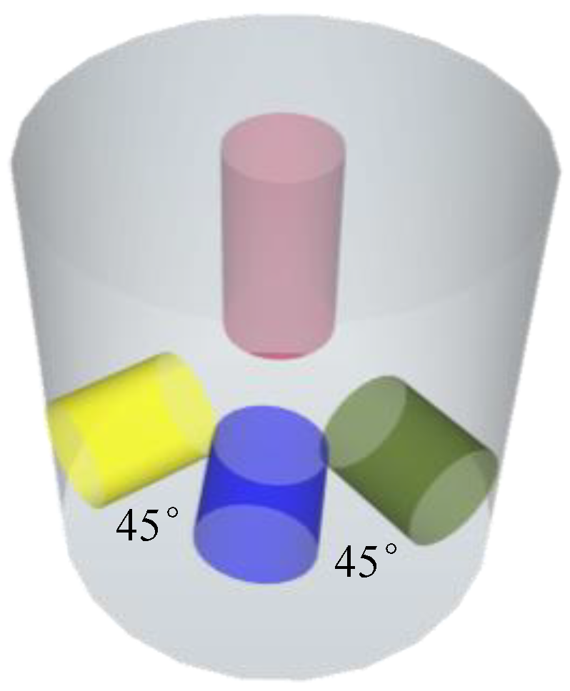
The Kaiser effect-based in situ stress testing assumes that the vertical direction is one of the principal stress directions. Vertical core samples are drilled along the direction of the vertical wellbore, and the vertical in situ stress at the coring point can be calculated based on the Kaiser point stress of the vertical core sample. Three horizontal core samples are drilled at 45° intervals in the horizontal plane, and the minimum and maximum horizontal principal stresses can be calculated based on the Kaiser point stresses of these horizontal core samples.

Acoustic emission (AE) signals were monitored during compression using R6α sensors. The Kaiser effect threshold was identified when AE activity surged at historical maximum stress. System parameters: 38 dB threshold, 50 μs hit duration, 2048 sampling points, 0.1 s interval, and 79.43 V threshold voltage. The test results are shown in

Table 1. Comparison table of in situ stress testing results.

Sample	Depth	Vertical Stress σv/(MPa)	Maximum Horizontal Principal Stress σH/(MPa)	Minimum Horizontal Principal Stress σh/(MPa)	Wellpoint Shut-In Pressure/(MPa)	Deviation Value
D17	4180	111.82	101.03	72.61	76.26	−4.79%
D001	4213	107.82	102.24	82.04	75.54	8.60%
D13	4004	106.38	96.05	78.21	/	/
D13	4210	102.08	105.59	75.14	77.91	−3.56%
D15	4250	104.82	105.50	75.14	76.40	−1.65%
D13	4211	103.68	98.80	69.96	/	/

.

Six sets of core samples yielded in situ stress ranges: maximum horizontal principal stress (σ_H): 96.05–105.59 MPa; minimum horizontal principal stress (σ_h): 69.96–82.04 MPa; vertical stress (σ_v): 102.08–111.82 MPa; and horizontal stress difference: 17.84–30.36 MPa (mean 26.02 MPa).

Data validation against shut-in pressure measurements showed −4.97%~8.60% deviation in σ_h, confirming method reliability.

3. Numerical Inversion of In Situ Stress Field

The in situ stress model of a reservoir is a primary tool for the quantitative analysis of in situ stress in oil and gas reservoirs. For single-well in situ stress studies, the magnitude and orientation of in situ stress can be calculated based on core testing and field logging data. However, for large-scale oil and gas reservoirs, the linear stress characteristics derived from single-well studies are insufficient to represent the distribution of in situ stress across the reservoir. Consequently, three-dimensional (3D) numerical inversion modeling has gradually emerged as a key method for analyzing in situ stress in oil and gas reservoirs.

The BKQ Formation reservoir exhibits significant lateral heterogeneity in rock mechanical properties. The field-measured in situ stress data reveal pronounced fault-induced disturbances, where major faults substantially alter local stress regimes and potentially influence hydrocarbon migration patterns. An integrated workflow combining geological modeling, in situ stress measurements, and numerical simulations was developed to establish a high-fidelity in situ stress analysis model for fault-affected zones to quantify these perturbations.

3.1. Matrix–Fault Coupled Modeling

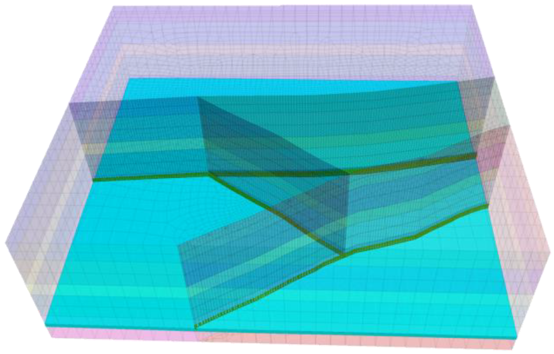
A stratigraphic model was constructed in Petrel using well logs, dynamic–static parameter conversion models, and regional geological data. Layer point clouds were exported and reconstructed in Rhino, where mesh surfaces were generated through curtain extraction operations. Ten stratigraphic horizons (T₁b₁₁ to T₁b₃₃) were integrated into a 3D geological entity, segmented by three fault planes into four structural blocks.

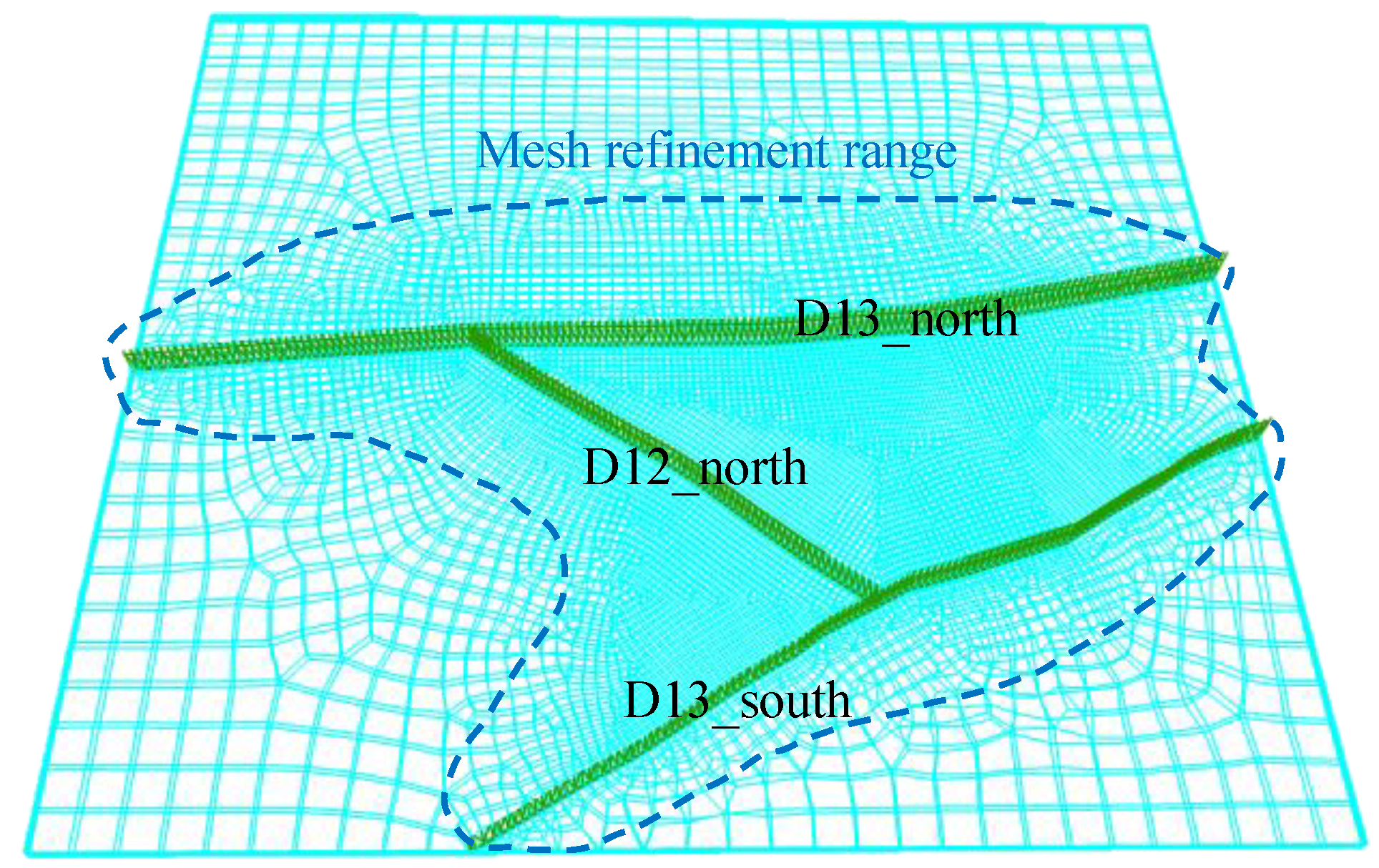
The initial mesh generated by Rhino’s native tools was refined using Griddle, particularly near faults, producing an f3grid format model for FLAC^3D6.0 analysis. The final grid spans −3925–−4441 m depth, covering 217.31 km² (15.689 km × 13.8509 km) with 2,016,735 nodes and 3,641,285 elements (Figure 4).

Based on the modeling approach of continuous reservoir matrix and discontinuous faults, the continuous matrix is represented by solid elements. Given that the rock exhibits significant elastic deformation characteristics during triaxial compression tests, a linear elastic constitutive model is adopted for the reservoir matrix units. The primary elastic parameters include Young’s modulus, Poisson’s ratio, and density. The mechanical parameters for the reservoir matrix units are assigned using continuous mechanical parameter data derived from acoustic well logging, which are optimized through dynamic–static Young’s modulus and Poisson’s ratio conversion relationships. The overburden density in the computational model is obtained by integrating well logging density data with depth.

To achieve reliable and reasonable parameter estimation between limited well logging data points, this study adopts the Kriging interpolation method as a robust tool for defining data between well locations. By systematically collecting and preprocessing well logging data, and thoroughly analyzing the spatial relationships and variability among well locations, the Kriging method is applied to perform precise interpolation calculations. This method explicitly accounts for the spatial correlation and continuity of the data, leveraging the inherent relationships between neighboring data points to produce more accurate estimations. Through a weighted averaging process, the method derives estimated values at interpolation points, effectively constructing a continuous and spatially coherent parameter field. This approach not only enhances the accuracy of the interpolated data but also provides a solid foundation for assigning parameters to the geomechanical model of the entire study area. By ensuring a more accurate and spatially consistent representation of geological and mechanical properties, the Kriging-based interpolation method significantly improves the reliability of the geomechanical model, supporting more informed decision-making in reservoir characterization and management.

For the discontinuous fault sections, the ‘separate’ command is used to define interface contact elements to simulate the faults (Figure 5). Three major faults within the study area are individually defined, with the faults modeled as zero-thickness elements. FLAC^3D6.0 interface elements are utilized to simulate fault discontinuity, incorporating Coulomb slip constitutive laws to capture the frictional behavior and potential slip along the fault surfaces. This approach allows for the realistic representation of fault mechanics, including shear stress accumulation, slip displacement, and stress redistribution, providing a detailed understanding of fault-related deformation and its impact on the reservoir. Interface parameters followed study [23]: cohesion C and friction angle φ equals 0.5–0.8× host rock value. Normal and shear stiffness values (K_n and K_s) were calculated as follows:

$$K_{\mathrm{n}}={\mathrm{K}}_{\mathrm{s}}={\displaystyle \frac{1}{20}}\left({\displaystyle \frac{K+\frac{4}{3}G}{\Delta Z_{\min }}}\right)$$

(8)

3.2. Stress Field Inversion

The gravitational stress field in the reservoir is primarily derived from the self-weight equilibrium of the overlying strata, which generates vertical stress due to the cumulative weight of the rock layers. The overburden pressure was calculated by integrating well logging density data with depth, providing a continuous profile of vertical stress distribution across the reservoir. The tectonic stress field, on the other hand, was determined based on the regional structural settings of the MH area, which is characterized by bidirectional compression from two major orogenic belts: the North Tianshan orogenic belt, exerting northward thrusting forces, and the West Junggar orogenic belt, exerting eastward thrusting forces. These tectonic forces significantly influence the horizontal stress components in the reservoir.

Kaiser effect measurements, conducted to assess the in situ stress state, revealed that the orientations of the principal stresses were closely aligned with the model axes (X: west–east and Y: south–north), with negligible vertical shear stresses observed. This alignment indicates a relatively stable stress regime dominated by horizontal compression.

The inversion procedure employed to reconstruct the in situ stress field incorporated both the gravitational stress field and the bidirectional tectonic stress field. This was achieved through the following detailed steps:

a.

Gravitational stress equilibrium: Applied normal displacement constraints to model base and lateral boundaries; imposed gravitational acceleration g = 9.8 m/s²; computed equilibrium state; and recorded stress at coring points.

b.

X-direction tectonic stress loading: Removed western boundary constraints; applied velocity boundary v = 2 × 10⁻⁴ m/s (West Junggar compression); executed 7400 calculation steps; reinstated displacement constraints; and performed 1000 equilibrium steps.

c.

Y-direction tectonic stress loading: Maintained X-direction constraints; removed southern boundary constraints; applied equivalent velocity (North Tianshan compression); executed 6200 calculation steps; reinstated constraints; and finalized with 1000 equilibrium steps.

Stress evolution was monitored via FLAC^3D6.0’s history command. Stress increments from tectonic loading were isolated using superposition principles:

$$\sigma =0.97{\sigma }_{\mathrm{ZZ}}+12.06{\sigma }_{\mathrm{XX}}+5.87{\sigma }_{\mathrm{YY}}$$

(9)

where σ_ZZ, σ_XX, and σ_YY represent gravitational, X-direction tectonic, and Y-direction tectonic stress components, respectively. Multivariate linear regression with least squares optimization calibrated tectonic stress coefficients, achieving <5% deviation between simulated and measured stresses through iterative refinement.

4. Result Analysis

A comparison between numerical simulations and field-measured in situ stresses demonstrates an error range of −2.96% to 9.07% for principal stresses, validating the reliability of the inversion methodology. Notably, acoustic emission testing did not account for core unloading time effects, potentially causing a minor underestimation of historical stresses. The numerical simulation results of key points and the comparison of acoustic emission test results are shown in

Table 2. Comparison table for acoustic emission method of in situ stress testing.

Well Number	Measured Data		Simulated Data		Deviation Value
	σH (MPa)	σh (MPa)	σH (MPa)	σh (MPa)	σH	σh
D13	105.59	75.14	102.53	74.61	2.98%	0.71%
D17	101.03	72.61	102.86	74.76	−1.81%	−2.96%
D15	105.5	75.14	102.8	75.01	2.62%	0.17%
D001	102.24	82.4	103.83	74.93	−1.56%	9.07%

.

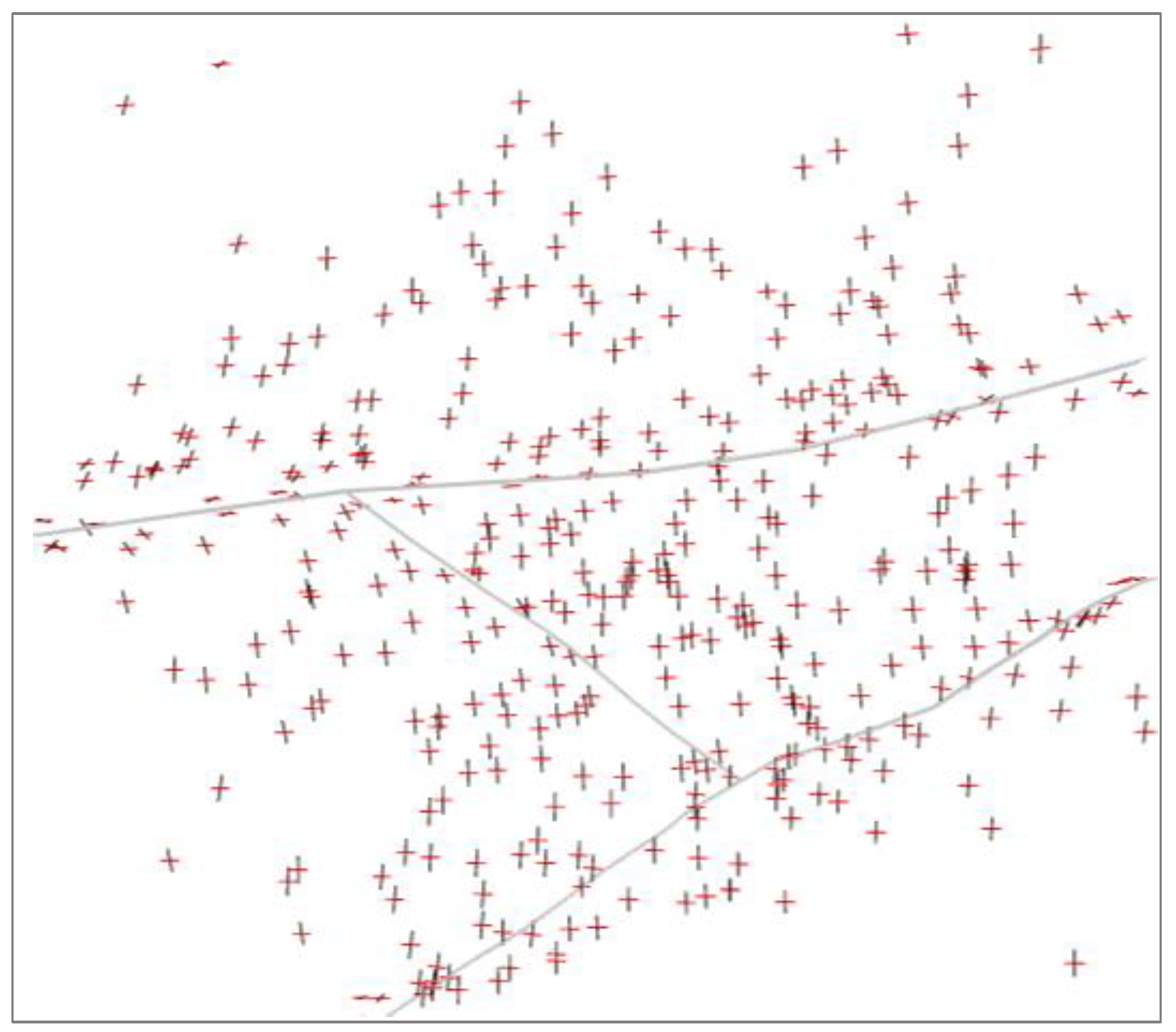
The simulation results of the direction of in situ stresses are shown in Figure 6. Red vectors denote maximum horizontal principal stress (σ_H), while black vectors represent minimum horizontal principal stress (σ_h). The overall σ_H orientation aligns approximately E-W, with localized deflections near faults. Previous studies [30] indicate maximum stress deflection occurs when faults intersect σ_H at 30°~60°, with deflection directions parallel to fault strikes. In this study, the D13 Well North and South Faults (subparallel to E-W) exhibit limited deflection due to small intersection angles.

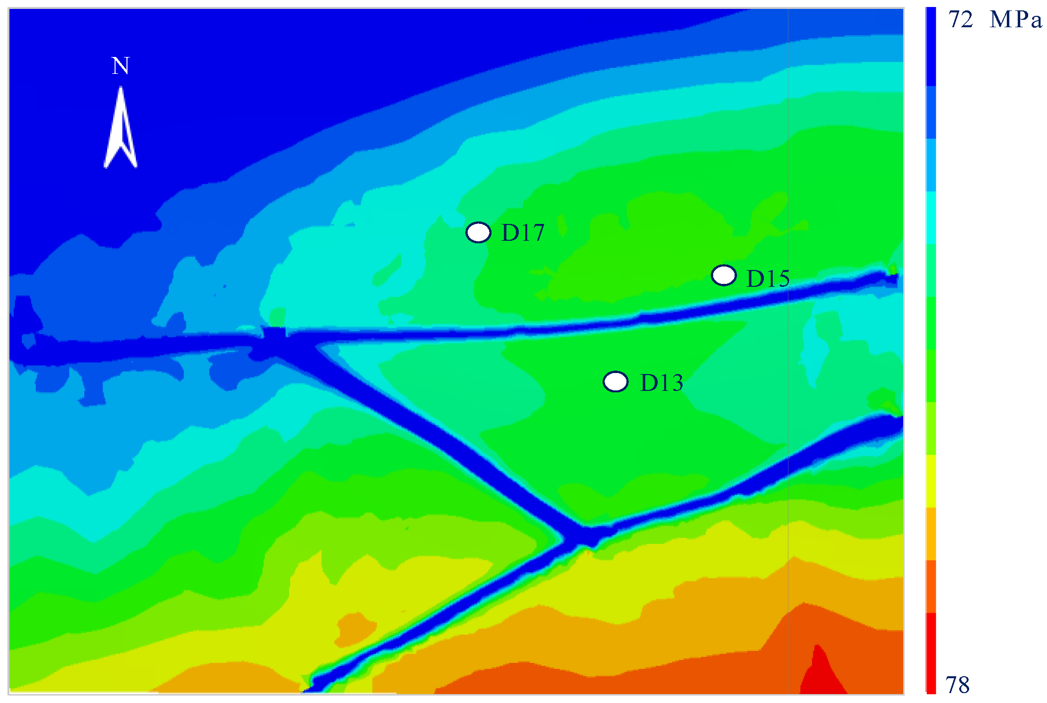
The simulation results of the minimum principal stress are shown in Figure 7. The σ_h distribution range is 70–78 MPa, increasing southeastward with maximum values in the southeastern model domain. Stress reductions (up to 7.6 MPa) occur near major faults, particularly at the intersection of the D12 Well North Fault and D13 Well North Fault.

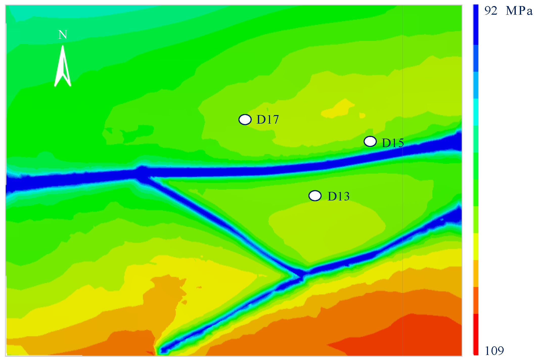
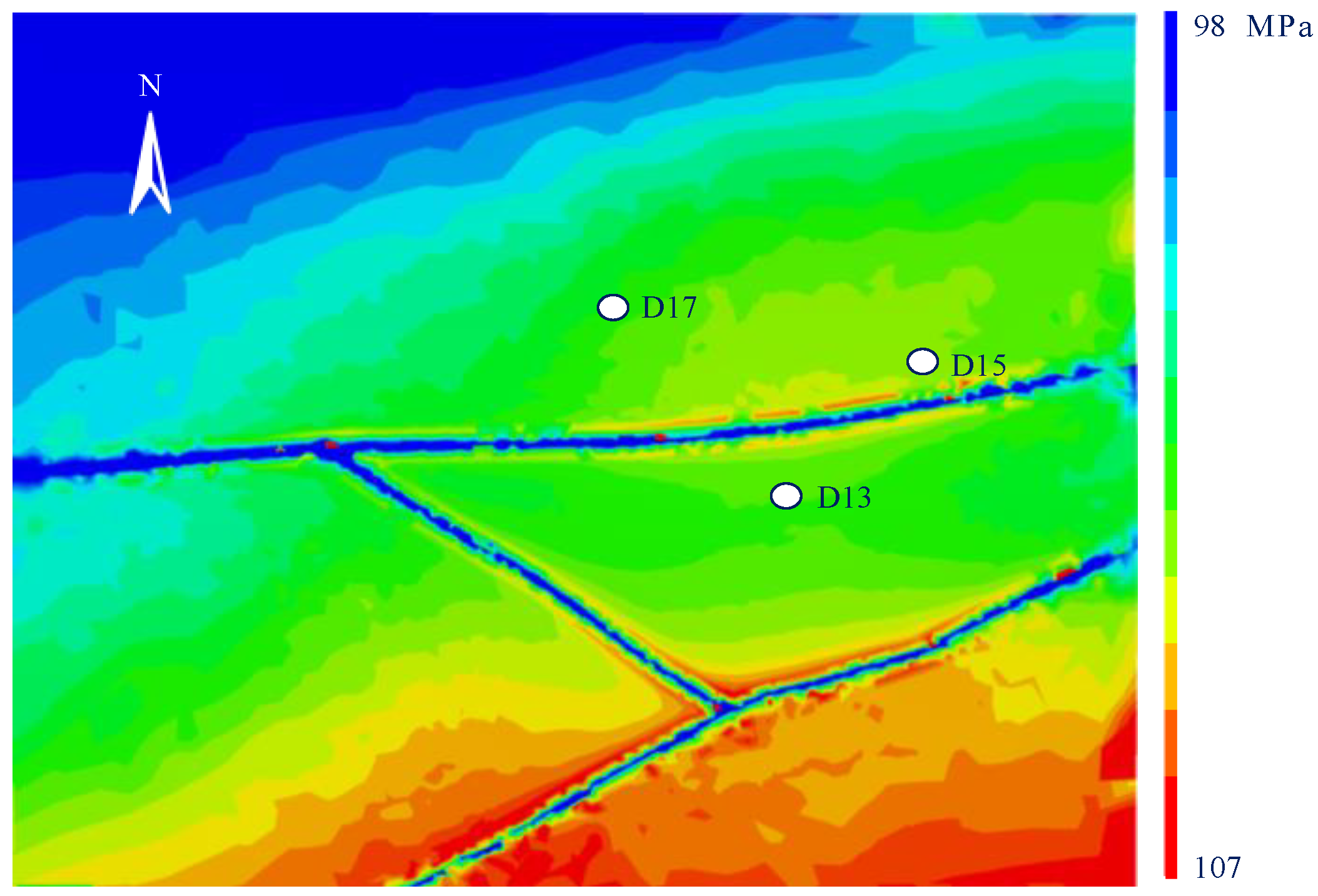
The simulation results of the maxmum principal stress are shown in Figure 8. The σ_H distribution spans 96–109 MPa, showing similar southeastward intensification. Fault-induced stress reductions reach 22.3 MPa at the D12-D13 fault intersection, highlighting stronger perturbation effects on σ_H.

Vertical stresses (Figure 9) range from 97 to 106 MPa, with maximum values in the southeastern corner. Faults induce stress concentrations: a 13.1 MPa reduction on fault inner walls versus localized increases on outer walls.

Key observations:

• All principal stresses exhibit NW-SE increasing gradients: σ_h 6 MPa differential; σ_v 9 MPa differential; and σ_H 13 MPa differential.
• Tectonic forces disproportionately affect σ_H, reflecting directional stress coupling.
• Faults induce asymmetric stress perturbations: σ_H: maximum reduction (22.3 MPa) at fault intersections and σ_v: stress concentration contrast between fault walls.

5. Discussion

The study area contains three major faults (from north to south): the D13 Well North Fault (D13_north), D12 Well North Fault (D12_north), and D13 Well South Fault (D13_south). D13_north and D13_south are first-order reverse faults with E-W and SW-NE strikes, respectively, while D12_north is a second-order accommodation strike-slip fault with NW-SE orientation (Figure 10 and Figure 11).

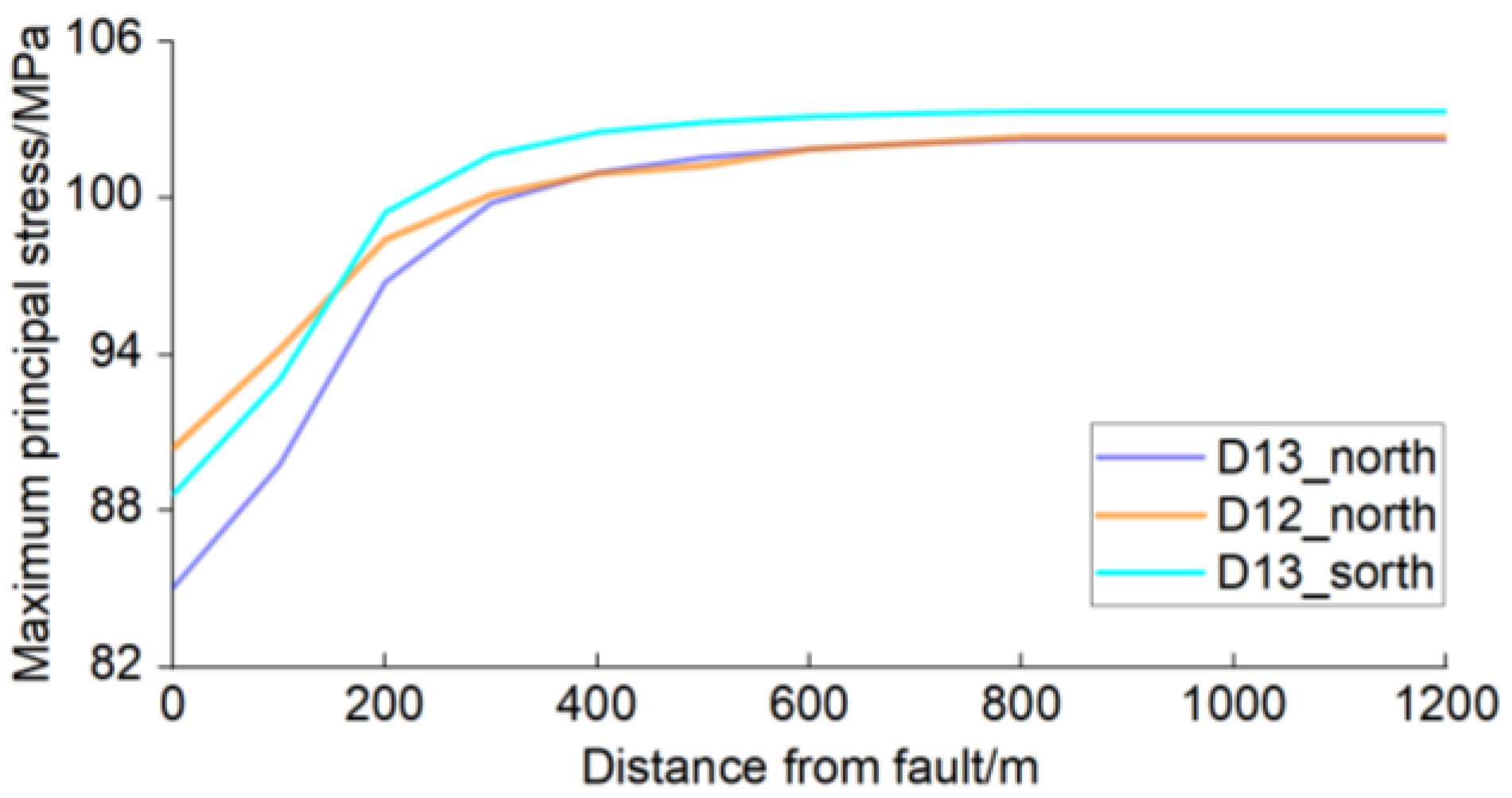
Background σ_H increases southward: undisturbed σ_H magnitudes follow D13_south > D12_north > D13_north. Fault-induced σ_H reductions rank as follows: D13_north (17.60 MPa) > D13_south (14.79 MPa) > D12_north (12.84 MPa). Previous studies [31] confirm that the fault scale controls the disturbance range, aligning with our numerical results showing that larger faults induce broader perturbations.

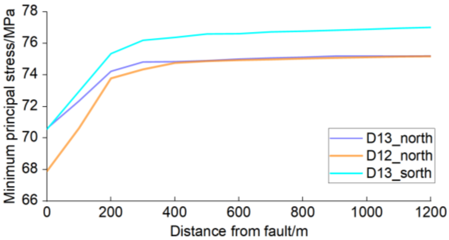
Undisturbed σ_h magnitudes similarly increase southward (D13_south > D12_north > D13_north). Fault-induced σ_h reductions are as follow: D12_north (7.29 MPa) > D13_south (6.46 MPa) > D13_north (4.60 MPa).

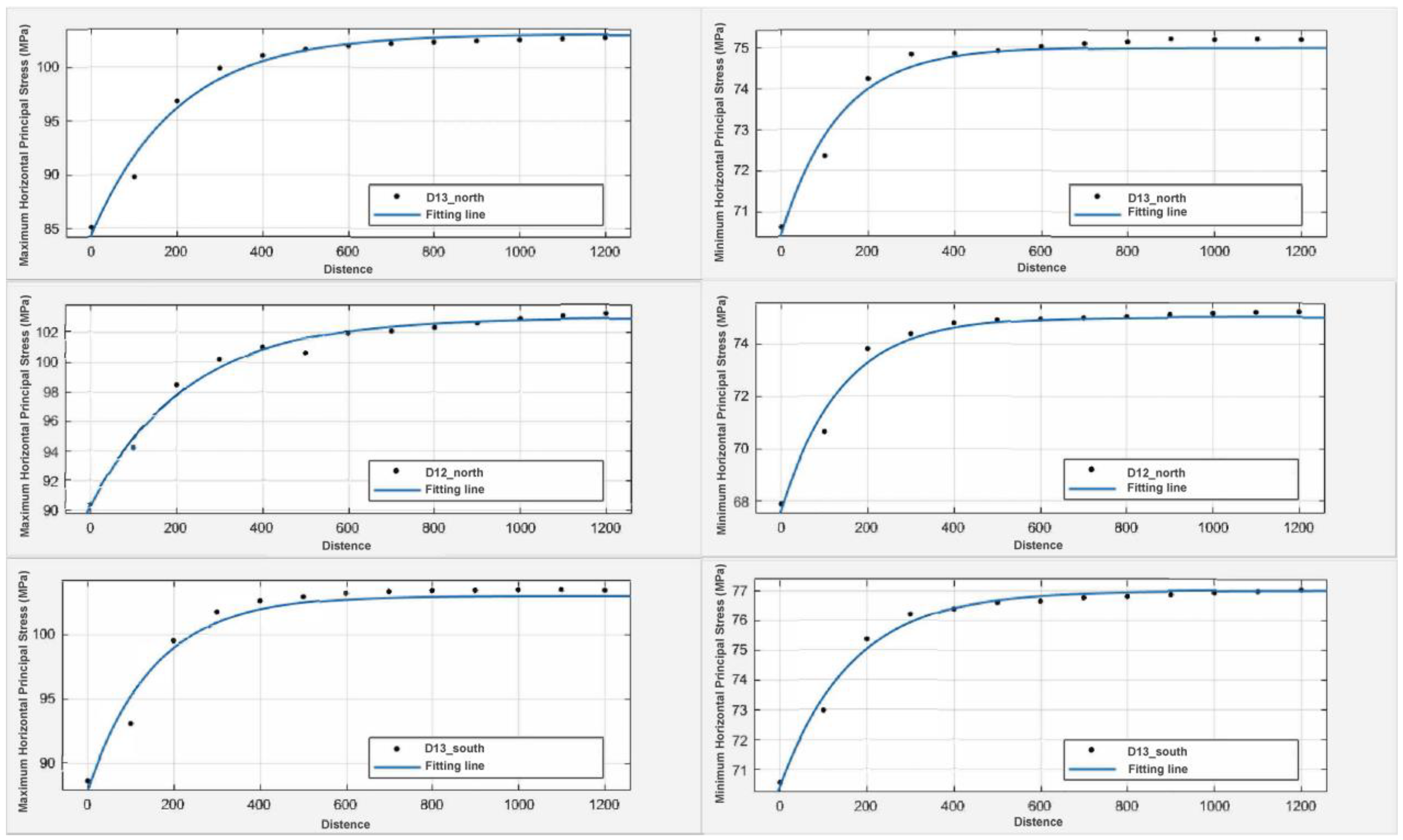
Both σ_H and σ_h recover 80% of the background values within 200 m from faults. To quantify perturbation ranges, exponential decay functions were applied, f(x) = ae^bx, where a (stress perturbation intensity) and b (decay rate) characterize fault effects (Figure 12).

Fitted parameters in

Table 3. Fitting coefficient table.

Fault Number	D13_north σH	D13_north σh	D12_north σH	D12_north σh	D13_south σH	D13_south σh
a	18.63	4.53	12.66	7.32	15.09	6.55
b	0.005001	−0.007497	−0.004363	−0.007176	−0.006506	0.006009

and

Table 4. Distances of Stress perturbation boundary.

Fault Number	D13_north σH	D13_north σh	D12_north σH	D12_north σh	D13_south σH	D13_south σh
Distance (m)	277.20	184.91	317.74	193.18	213.08	230.70

reveal that σ_H perturbations persist over longer distances than σ_h. D12_north exhibits the largest σ_H disturbance range (317.74 m at 25% residual perturbation).

These results align with field observations by Brudy [32] and Tamagawa [33], who reported ~200 m stress perturbation boundaries in hydrocarbon reservoirs. To mitigate stress discontinuity risks, a 320 m buffer from faults is recommended for development safety.

While the model demonstrates high accuracy within the study area, key assumptions include the following:

• Elastic constitutive behavior neglecting plastic deformation;
• Simplified bidirectional tectonic loading without regional curvature effects;
• Homogeneous lithology interpolation between wells.

These constraints suggest cautious extrapolation to reservoirs with pronounced lithological heterogeneity or viscoelastic creep behavior.

6. Conclusions

This study investigated fault-induced stress perturbations in the BKQ Formation of the MH area, China, through numerical in situ stress inversion modeling. The key conclusions are as follows:

• The numerical model demonstrates high accuracy, with deviations ranging from −2.96% to 9.07% deviations between simulated and measured stresses, validating the multivariate regression analysis methodology.
• In situ stresses exhibit NW-SE increasing gradients:
  Minimum horizontal principal stress (σ_h): 70 –78 MPa;
  Maximum horizontal principal stress (σ_H): 96–109 MPa;
  Vertical principal stress (σ_v): 97–106 MPa.

The dominant σ_H orientation aligns E-W, with minor deflections (<15°) near faults.

• Faults reduce principal stress magnitudes asymmetrically:
  Reverse faults induce stronger σ_H reductions (up to 17.60 MPa) than strike-slip faults;
  Stress recovery reaches 75% of the background values within 200 m from faults.
• Exponential fitting quantifies fault disturbance ranges:
  The 25% residual stress perturbation boundary spans 184.91–317.74 m from faults;
  The maximum disturbance range (317.74 m) occurs at D12_north fault for σ_H.

Overall, these findings provide critical constraints for optimizing well placement and hydraulic fracturing designs in faulted reservoirs.

Future research will explore hybrid physics–AI frameworks [34] to address uncertainties in faulted reservoirs. Integrating machine learning with continuum–discontinuum models could enhance stress prediction under sparse data conditions, particularly for complex fault networks.