Applications for Predicting Cracking Outlet Temperatures for Ethylene Cracker Furnaces Based on the GAC-BiLSTM-AM Method

Abstract

In order to achieve a good generalization ability across different prediction tasks and ensure the reliability of prediction results, this paper proposes a GAC-BiLSTM-AM prediction method based on ensemble learning. This method employs a dual-channel convolutional neural network to comprehensively extract and integrate sample features, which are then input into a composite analysis module consisting of a bidirectional long short-term memory, an attention mechanism, and a fully connected layer to achieve in-depth analysis and processing of information, jointly constructing an efficient base learner. Meanwhile, during the parameter iteration tuning process of the base learner, a mistake correction mechanism is introduced to dynamically adjust sample weights in order to correct potential attention biases, and further combined with the gold rush optimizer to optimize the key structural parameters of the model. The application evaluation in multiple benchmark prediction tasks confirms that the GAC-BiLSTM-AM method possesses excellent generalization performance.

1. Introduction

Prediction technology is a comprehensive data analysis method, which aims to reveal and model the underlying patterns of events and make scientific inferences about future trends by carefully exploring historical data, current trends, established patterns, and domain knowledge. Currently, prediction technology is widely used in the fields of stock prices, traffic flow, air temperature, and power loads [1,2,3,4].

Time-series data play a crucial role in current forecasting tasks. This type of data is typically represented as an ordered sequence that records the results of observations or measurements of a process at fixed time intervals [5]. Additionally, cross-sectional data also play a key role in predictive analytics. Traditional statistical forecasting methods, such as autoregressive integrated moving average (ARIMA) [6], exponential smoothing (ES) [7], and Holt–Winters methods [8], primarily rely on difference operations and moving averages to capture the trends in time-series data. However, their linear assumptions often struggle to model the nonlinear coupling relationships that are common in industrial data. In contrast, machine learning techniques, especially deep learning algorithms, are capable of delving into the complex structures and dynamic characteristics of the data, thus addressing nonlinear modeling issues more effectively.

Currently, the mainstream deep prediction models are primarily based on recurrent neural networks (RNN) and long short-term memory networks (LSTM) as their core. These model temporal dependencies through the recursive updating mechanism of hidden state vectors; however, when dealing with long input sequences, the RNN is affected by the chain rule and prone to problems such as gradient explosion or vanishing [9,10]. LSTM mitigates this situation by introducing a gating mechanism and cellular states [11], but a single LSTM still suffers from problems such as solidification of hidden state dimensions, insufficient local feature capture, and low computational efficiency.

In order to overcome the representation bottleneck of single models, Lu et al. [12] proposed a CNN-LSTM cascaded model, which first utilizes convolutional kernels to extract local feature information from the data and then inputs this into the LSTM to capture temporal dynamics, achieving relatively outstanding performance, although there is still potential for improvement. Rai et al. [13] built upon this by introducing a bidirectional long short-term memory (BiLSTM) in place of LSTM, allowing the model to consider both the forward evolutionary characteristics and reverse dependencies of the data, thereby achieving a more comprehensive information analysis. Kavianpour et al. [14] further integrated the attention mechanism (AM) to dynamically focus on key time steps, further enhancing the model’s information recognition capabilities. However, there are still problems such as insufficient generalization ability and difficulty in parameter selection.

On the other hand, Wu et al. [15] attempted to combine the AdaBoost algorithm with LSTM by integrating the prediction results of each base learner through weighted integration, allowing the model to take a multi-perspective view of the problem, enhancing the comprehensiveness of the analysis. Yaprakdal [16] and Busari et al. [17] further confirmed the effectiveness of the ensemble learning strategy through experiments. However, it cannot be ignored that using a single model as the base learner results in a significant consumption of computational resources.

Given the existing research and challenges, we attempt to fuse the deep composite model with the concept of ensemble learning. Meanwhile, we introduce a dual-channel convolutional neural network, a mistake correction mechanism, and the gold rush optimizer to further optimize the model’s information processing capabilities, thereby achieving superior generalization performance. It should be noted that this paper is an expansion of our already accepted conference paper titled “The GAC-BiLSTM-AM Method and Its Application to the Prediction of Cracking Outlet Temperature in Ethylene Cracking Furnaces” [18], with the expanded content accounting for no less than thirty percent.

2. Background Knowledge and Methods

2.1. Convolution Neural Network (CNN)

CNN is a kind of feed forward neural network proposed by Lecun et al. [19] in 1989. The network simulates the way the human visual system processes visual information. The core idea is to extract and represent the multi-level features of the input data through the organic combination of internal functional modules, which is currently widely applied in the fields of face recognition, autonomous driving, bioinformatics, among others [20], and it mainly consists of three parts: a convolutional layer, pooling layer, and fully connected layer [21]. Among them, the convolutional layer is responsible for feature extraction, and each convolutional layer contains a set of learnable filters, which follow the principles of local connectivity and weight sharing; the pooling layer is responsible for feature selection, which reduces the dimension of the data; and the fully connected layer, which is usually located at the end of the neural network, is responsible for the integration of features. Since the convolution operation of CNN can effectively deal with the local correlation of the data, the use of one-dimensional convolution to extract data features in prediction tasks can help neural networks with a memory mechanism to better address long-term dependency issues.

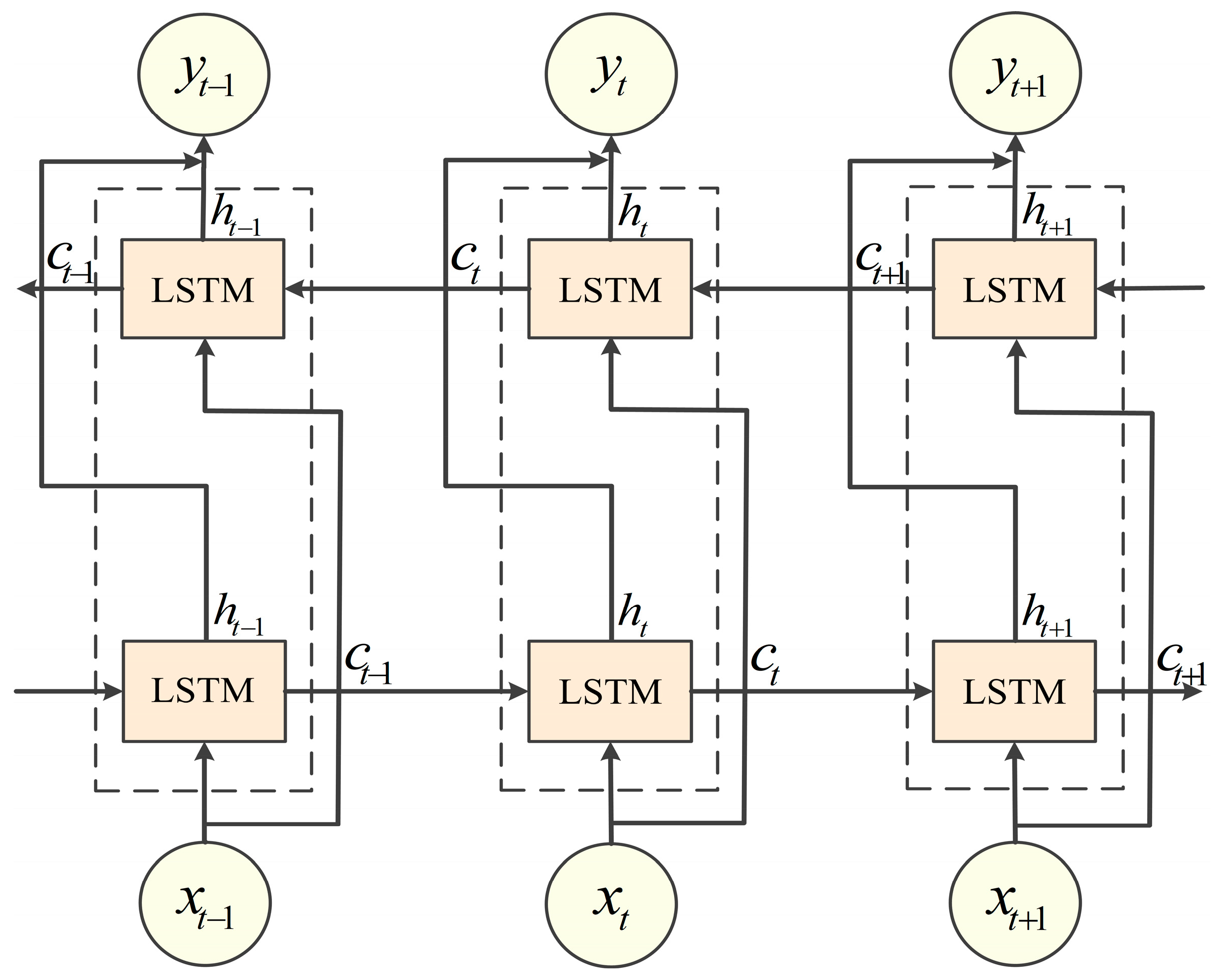
2.2. Bidirectional Long Short-Term Memory (BiLSTM)

In order to alleviate the long-term dependency problem of traditional recurrent neural networks, Sepp Hochreiter and Jürgen Schmidhuber [22] proposed LSTM in 1997. LSTM realizes the effective processing of sequence data through cell states and three types of gate structures. Building on this, BiLSTM was subsequently proposed, consisting of two LSTM layers running in parallel with opposite directions of information transfer. This allows BiLSTM to process data in both directions simultaneously, thereby enhancing its ability to understand and interpret sequences. The structure of BiLSTM is shown in Figure 1. Siami-Namini et al. [23] conducted a comparison across multiple datasets and found that the prediction accuracy of BiLSTM was improved. It was enhanced by an average of 37.78% compared to LSTM. Given the advantages of BiLSTM in handling sequential data, we employ this technique in our study to obtain better prediction performance. For example, we utilize BiLSTM’s bidirectional information flow to jointly model the historical time-series characteristics of multiple variables (e.g., temperature, humidity, and wind speed) and their inter-temporal dependencies, thereby accurately capturing the dynamic interaction patterns among the variables. In terms of stock price prediction, we analyze the influence of historical data on current prices using BiLSTM’s forward layer and reveal the market sentiment implied by current price fluctuations with the reverse layer, thereby gaining a more comprehensive understanding of the long-range dependencies within the price series.

2.3. Attention Mechanism (AM)

The attention mechanism is inspired by a human’s visual perception of the environment. When people make visual observations, the visual system will focus on the local area (key area) and, with the large amount of attention resources invested in this area, quickly obtain the required high-value information. Similarly, the attention mechanism will pay more attention to the important information, and the unimportant information is ignored, which is implemented through a weighted processing approach, typically divided into the following three stages [24]:

(1)

Calculate the correlation between Query (output feature) and Key (input feature) as shown in Equation (1):

$$s_t=\tanh \left(W_h{h}_t+b_h\right)$$

(1)

where $W_h$ is the weight of the attention mechanism, $b_h$ is the bias of the attention mechanism, and $h_t$ is the input vector.

(2)

Normalize the obtained $s_t$ scores to maintain the value range between 0 and 1, as shown in Equation (2):

$$a_t={\displaystyle \frac{\exp \left(s_{t}v\right)}{{\displaystyle {\sum }_t\exp \left(s_{t}v\right)}}}$$

(2)

where $v$ is the attention value.

(3)

Based on the weighting coefficients $a_t$, perform a weighted summation to arrive at the final attention value, as shown in Equation (3):

$$s={\displaystyle {\sum }_t{a}_t{h}_t}$$

(3)

By assigning different weights to information, the attention mechanism allows the model to focus on the important parts of the data. This mechanism has been applied in various fields such as image captioning, behavioral analysis, earthquake forecasting, etc. [25,26,27]. In this paper, we assign weights and sum the output of BiLSTM in the time dimension with the help of the attention mechanism to effectively highlight the key time steps that have a significant impact on the final prediction results to help the model accurately identify and process the core information, and further improve the accuracy of the prediction.

2.4. Gold Rush Optimizer (GRO)

The gold rush optimizer is a meta-heuristic algorithm proposed by Kamran Zolf [28] in 2023. The algorithm simulates the gold panning process carried out by gold miners during the gold rush era, which mainly consists of three parts: migration, mining, and collaboration. The algorithm starts by first generating a batch of gold miners randomly, and each of them has the corresponding fitness value (the total amount of gold that can be mined under the current location). When the gold miners find other gold mines, they will change the location. At the same time, because the location of the best gold mine belongs to an unknown state, the algorithm approximates the location of the best gold miner as the location of the best gold mine, and the formula of the migration process is as follows:

$${\overrightarrow{D}}_1={\overrightarrow{C}}_1\cdot {\overrightarrow{X}}^{*}\left(t\right)-{\overrightarrow{X}}_i\left(t\right)$$

(4)

$${\overrightarrow{Xnew}}_i\left(t+1\right)={\overrightarrow{X}}_i\left(t\right)+{\overrightarrow{A}}_1\cdot {\overrightarrow{D}}_1$$

(5)

$${\overrightarrow{A}}_1=1+l_1\left({\overrightarrow{r}}_1-{\displaystyle \frac{1}{2}}\right)$$

(6)

$${\overrightarrow{C}}_1=2{\overrightarrow{r}}_2$$

(7)

$$l_e={\left({\displaystyle \frac{{\max }_{iter}-iter}{{\max }_{iter}-1}}\right)}^e\left(2-{\displaystyle \frac{1}{{\max }_{iter}}}\right)+{\displaystyle \frac{1}{{\max }_{iter}}}$$

(8)

where ${\overrightarrow{X}}^{*}$ is the location of the best gold mine, ${\overrightarrow{X}}_i$ is the location of the $i$-th gold miner, $t$ is the current iteration number, ${\overrightarrow{Xnew}}_i$ is the new position of the $i$-th gold miner, ${\overrightarrow{r}}_1, {\overrightarrow{r}}_2$ are random vectors with values ranging from 0 to 1, $l_1$ is defined by equation (8), ${\max }_{iter}$ is the maximum number of iterations, and $iter$ is the current number of iterations.

During the gold panning process, each gold miner tries to mine as much gold as possible from their own panning area. The formula for the mining process is as follows:

$${\overrightarrow{D}}_2={\overrightarrow{X}}_i\left(t\right)-{\overrightarrow{X}}_r\left(t\right)$$

(9)

$${\overrightarrow{Xnew}}_i\left(t+1\right)={\overrightarrow{X}}_r\left(t\right)+{\overrightarrow{A}}_2\cdot {\overrightarrow{D}}_2$$

(10)

$${\overrightarrow{A}}_2=2l_2{\overrightarrow{r}}_1-l_2$$

(11)

where ${\overrightarrow{X}}_r$ is the location information of a gold miner randomly selected among the remaining gold miners after removing the $i$-th gold miner, and $l_2$ is also defined by Equation (8).

In order to improve the efficiency of the search for gold in a limited time, sometimes, it is necessary for more than one person to work as a team, and the formula of the cooperation process between members is as follows:

$${\overrightarrow{D}}_3={\overrightarrow{X}}_{g2}\left(t\right)-{\overrightarrow{X}}_{g1}\left(t\right)$$

(12)

$${\overrightarrow{Xnew}}_i\left(t+1\right)={\overrightarrow{X}}_i\left(t\right)+{\overrightarrow{r}}_1\cdot {\overrightarrow{D}}_3$$

(13)

where ${\overrightarrow{X}}_{g1}, {\overrightarrow{X}}_{g2}$ are the location information of the two gold miners randomly selected among the remaining gold miners after removing the $i$-th gold miner.

For all the above processes, the gold miner updates the position only if the gold content (fitness value) of the new position is better than the previous position; otherwise, the original position is kept unchanged, and the modeling formulation of the minimization problem is as follows:

$$\hspace{1em}\hspace{1em}{\overrightarrow{X}}_i\left(t+1\right)=\overrightarrow{Xne{w}_i}\left(t+1\right) if\hspace{1em}f\left(\overrightarrow{Xne{w}_i}\left(t+1\right)\right)<f\left({\overrightarrow{X}}_i\left(t\right)\right)$$

(14)

The gold rush optimizer offers advantages such as fast convergence speed and the capability of achieving global optimization. Optimizing the key structural parameters of the model with this algorithm can yield superior results.

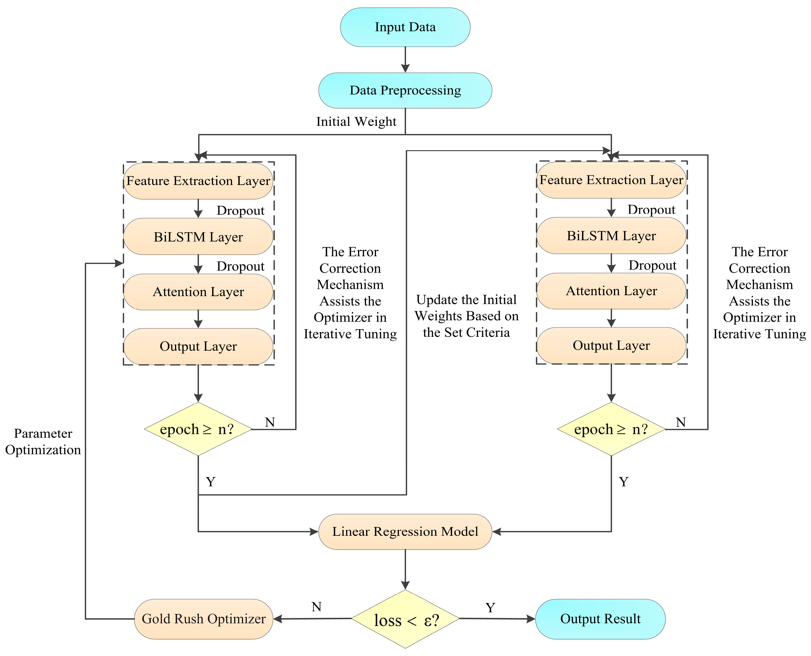
2.5. Model Framework

The overall architecture of the GAC-BiLSTM-AM model is shown in Figure 2.

Before training commences, the input data is preprocessed as follows: First, an appropriate imputation strategy is selected to handle missing values based on the data characteristics. Second, using the Pearson correlation coefficient, features that have a correlation coefficient of at least 0.19 with the target variable are selected as input features. Lastly, the input features are normalized with z-score normalization, retaining the mean and standard deviation. These preprocessing operations aim to improve data quality, reduce the impact of noise and outliers, and unify feature scales. The comparison of effects is shown in Figure 3. In the figure, the left side depicts the original feature data, while the right side shows the feature data after preprocessing.

The data are then transformed into a three-dimensional tensor $X\in R^{BTD}$ using the sliding window technique where $B$ is the batch size, $T$ is the time step, and $D$ is the feature dimension. The sample weights are initialized and fed into a dual-channel convolutional neural network to capture sample features, the bidirectional long short-term memory network, attention mechanism, and fully connected layers for further analysis and processing. Finally, the real results are obtained through inverse normalization. To prevent overfitting, Dropout is added after the convolutional module and the bidirectional long short-term memory network to achieve random inactivation of neurons.

During the iterative optimization process, the mistake correction mechanism assists the adaptive optimization algorithm in adjusting model parameters. The linear regression model maps the aggregated outputs of all base learners to the final result. The gold rush optimizer is used to search for the optimal values of four key structural parameters: the number of neurons in the BiLSTM hidden layer, the two independent Dropout discard rates, and the weight update interval value. The main reason for this is that having too many hidden layer neurons may cause the model to overfit, while too few may fail to adequately capture the complexity of the time series. If the Dropout discard rate is set too low, it will not effectively prevent overfitting; conversely, if set too high, it may lead to underfitting of the model. Similarly, if the weight update interval is too small, it will not effectively contribute to the model’s correction; if too large, it may introduce new attention biases. Only with appropriate parameter settings can the model be ensured to have good predictive performance. The search ranges are [20, 136], [0, 0.3], [0, 0.3], and [5, 20], respectively. These ranges were based on the parameter settings in multiple papers in related fields and were finalized with the specific needs of this study. The optimization goal of the gold rush optimizer in the experiment is to find the minimum cumulative sum of the four evaluation metrics. Throughout the optimization process, the number of neurons in the BiLSTM hidden layer and the weight update interval are rounded to integers when input into the model.

2.6. Dual-Channel Convolutional Neural Network

In the feature mining process, the model’s deep representation learning capability plays a crucial role in the accuracy of prediction results. Traditional single-layer one-dimensional convolutional neural networks have limitations in deep feature representation, making it difficult to fully capture the global information of the data. Especially when dealing with industrial data characterized by non-stationarity and strong coupling, it can easily lead to the loss of key information and degradation of representation capabilities. To address this issue, we propose a dual-channel convolutional neural network architecture, as shown in Figure 4. In this architecture, the single-layer one-dimensional convolution is responsible for capturing shallow feature information, while the three-layer stacked one-dimensional convolution focuses on mining deep abstract feature information. The two convolution modules work in collaboration to ensure the comprehensiveness and consistency of feature extraction. Furthermore, to overcome issues such as vanishing gradients, the ReLU activation function is used to introduce nonlinearity, ensuring that gradients can propagate effectively through the network. Finally, a fully connected layer is employed to integrate the extracted information, improving the computational efficiency of the model.

2.7. Mistake Correction Mechanism

During the process of iterative optimization of model parameters, adaptive optimization algorithms such as Adam can easily lead to implicit preference optimization issues due to the heterogeneity of sample prediction difficulty. This manifests as follows: the optimization process tends to quickly converge to local optima composed of easy-to-learn samples, while the gradient response to difficult-to-predict samples gradually diminishes. This phenomenon will result in two key deficiencies: 1. The model’s decision boundary is dominated by easy-to-learn samples, making it difficult to capture the tail characteristics of the data distribution. 2. The parameter update direction deviates from the global optimal trajectory, thereby weakening the model’s generalization ability. To address this optimization bias, we propose a mechanism for dynamically adjusting sample weights, with the following specific implementation details:

In the initial phase of training, which is the first 60% of the total number of iterations, all training samples are assigned equal weights. At this point, the adjustment of model parameters relies entirely on the action of the adaptive optimization algorithm, with the aim of quickly reducing the training loss. When the number of iterations reaches 60% of the total, in this and subsequent iterations, an additional judgment is made to determine if the current iteration count is divisible by a predefined weight update interval value. If the integer division condition is met, the weights of the samples with an absolute prediction error exceeding the dividing value for that round are increased, while the weights of other samples are decreased for use in the next iteration. The weight update formula is as follows:

$$o=S\left(D,Q_t\right)$$

(15)

$$\gamma =\delta -\left(t-\widehat{T}\right)\times \vartheta$$

(16)

$${\phi }_i=\left\{\begin{array}{ll}{Q}_{ti},\hfill & \left|o_i-f_i\right|>\gamma \hfill \\ 0,\hfill & \left|o_i-f_i\right|\le \gamma \hfill \end{array}\right.$$

(17)

$$\beta =\left\{\begin{array}{ll}{\displaystyle \frac{1}{2}}\ln \left({\displaystyle \frac{1-{\displaystyle \sum {\phi }_i}}{{\displaystyle \sum {\phi }_i}}}\right),\hfill & {\displaystyle \sum {\phi }_i}<0.5\hfill \\ {\displaystyle \frac{1}{2}}\ln \left({\displaystyle \frac{{\displaystyle \sum {\phi }_i}}{1-{\displaystyle \sum {\phi }_i}}}\right),\hfill & {\displaystyle \sum {\phi }_i}\ge 0.5\hfill \end{array}\right.$$

(18)

$$Q_{t+1}={\displaystyle \frac{Q_t}{{\displaystyle \sum Q_{ti}^{\prime }}}}\times \left\{\begin{array}{ll}{e}^{-\beta },\hfill & \left|o-f\right|\le \gamma \hfill \\ e^{\beta },\hfill & \left|o-f\right|>\gamma \hfill \end{array}\right.$$

(19)

where $S$ is the base learning model used, $D$ is the training dataset, $Q_t$ is sample weights for the $t$ iteration, $o$ is the prediction results, $\delta$ is the initial value, $t$ is the current iteration number, the value of $\widehat{T}$ is sixty, $\vartheta$ is the decrement, $\gamma$ is the dividing value, subscript $i$ is the $i$-th sample, $Q_{ti}$ is the weight of the $i$-th sample in the $t$ iteration, $f$ is the sample label, and $Q_{ti}^{\prime }$ is the weight of $Q_{ti}$ after updating.

If the integer division condition is not met, the sample weights from the previous iteration continue to be used, thereby assisting the adaptive optimization algorithm in adjusting the model parameters, ensuring that the model can give appropriate attention to samples that were not fully considered previously.

It is worth noting that, to ensure the denominator in Formula (18) is not zero, the initial value is set relatively small for all tasks. The denominator in Formula (19), being the sum of all weights after the sample weights are updated, will always be greater than zero.

3. Experiments and Results

The experimental process is divided into two stages: comparison and application. First, a comparative analysis of single-step and multi-step (five-step) prediction results is conducted on public and simulated data. In the experiment, the appropriateness of the chosen time step size directly affects the accuracy of the final results. When the time step is small, it is beneficial for the model to capture instantaneous changes in information, thus better reflecting the dynamic characteristics of the system. When the time step is large, it helps the model focus on the long-term trends and overall patterns in the data. After multiple experimental tests, we finally set the time step size as follows: for single-step prediction, the step size is 5, and for multi-step prediction, the step size is 20. In the experiments, the number of iterations for the model is 100, the loss function is MSE, the activation function is RELU, the optimizer is Adam, and the learning rate is 0.01. In the comparison stage, the average of ten evaluation metrics is used as the basis for measuring the performance of the model, with the standard deviation serving as auxiliary information. Furthermore, since the data used in the experiments may be subject to measurement errors, signal interference, and operational changes, leading to uncertainty and inaccuracy, fuzzy similarity or the Pearson correlation coefficient might be an effective solution [29,30]. In this paper, we choose to combine the Pearson correlation coefficient to filter out the features.

In the comparison phase, the model parameters for the other four compared methods are derived from the literature [24], as shown in

Table 1. Compare model parameters.

Parameters	Value
Convolution layer filters	64
Convolution kernel size	1
Number of hidden units	64

. Some of the parameters in our method are obtained through the gold rush optimizer, which seeks optimal values during a single-step prediction experiment on the first 10,000 data points of the Jena Climate Dataset, while other parameters are determined through multiple experimental tests.

3.1. Evaluation Metrics

We use four evaluation metrics, namely, mean absolute error (MAE), root-mean-square error (RMSE), coefficient of determination (R²), and symmetric mean absolute percentage error (SMAPE), to comprehensively assess the performance of the model. The reason for choosing these metrics is that they are widely recognized in the field of prediction and are able to evaluate the model’s performance from different perspectives, ensuring the comprehensiveness and accuracy of the assessment. In the model, the smaller the values of MAE, RMSE, and SMAPE, the smaller the deviation of the model-predicted value from the real one, and the higher the model fitting accuracy. The closer the R² value is to 1, the stronger the explanatory ability of the independent variables to the dependent variable in the regression analysis, and the better the model prediction effect. The formulas for the four evaluation indexes are shown below [31]:

$$MAE={\displaystyle \frac{1}{n}}{\displaystyle {\sum }_{i=1}^n\left|{\widehat{y}}_i-y_i\right|}$$

(20)

$$RMSE=\sqrt{{\displaystyle \frac{1}{n}}{{\displaystyle {\sum }_{i=1}^n\left({\widehat{y}}_i-y_i\right)}}^2}$$

(21)

$$R^2=1-{\displaystyle \frac{{\displaystyle {\sum }_{i=1}^n{\left({\widehat{y}}_i-y_i\right)}^2}}{{\displaystyle {\sum }_{i=1}^n{\left(y_i-\overline{y}\right)}^2}}}$$

(22)

$$SMAPE={\displaystyle \frac{1}{n}}{\displaystyle {\sum }_{i=1}^n\frac{\left|{\widehat{y}}_i-y_i\right|}{\left(\left|{\widehat{y}}_i\right|+\left|y_i\right|\right)/2}}\times 100\%$$

(23)

where $\widehat{y}$ is model prediction value, $y$ is sample true value, $\overline{y}$ is sample mean, and $n$ is number of prediction samples.

3.2. Public Data

3.2.1. Dataset Introduction and Model Parameter Settings

We used three different types of time series data as public datasets. Among them, the temperature dataset uses the Jena Climate Dataset and takes the first 10,000 pieces of data as well as the 51,264th piece of data to the 61,263th piece of data to form the T1 and T2 datasets. The oil temperature dataset uses the ETT-small-h1 under the Electric Transformer Dataset and takes the first 10,000 pieces of data to form the ETTh1 dataset, and the price dataset uses the two stocks indexed as 000001 and 000002 in the Shenzhen index in the Tushare financial data interface package, which are referred to as the S1 and S2 datasets. For single-step prediction, the ratio of training to testing data is 7:3 for all datasets, and for multi-step prediction, the ratio of training to testing data is still 7:3 for the T1, T2, and ETTh1 datasets, whereas for the S1 and S2 datasets, the last 3 pieces of data of the S1 dataset are removed first, and then the first 5500 pieces of data are taken for training and the last 2355 pieces of data are taken for testing, respectively. The GAC-BiLSTM-AM model parameter settings in the public dataset are shown in

Table 2. Parameters of the GAC-BiLSTM-AM model in public data.

Parameters	Value
	Single Step	Multistep
Single-layer convolution filters	77	77
Single-layer convolution kernel size	1	1
Three-layer convolution filters	19/38/77	19/38/77
Three-layer convolution kernel size	1	1
Full connection layer output size	77	77
First dropout rate	0	0
Number of hidden units in BiLSTM layer	77	77
Second dropout rate	0.000325415686	0.000325415686
Initial value	0.25	2.1
Decrement	0.005	0.02
Weight update interval value	11	11
Threshold	0.15	0.85

.

3.2.2. Result Analysis

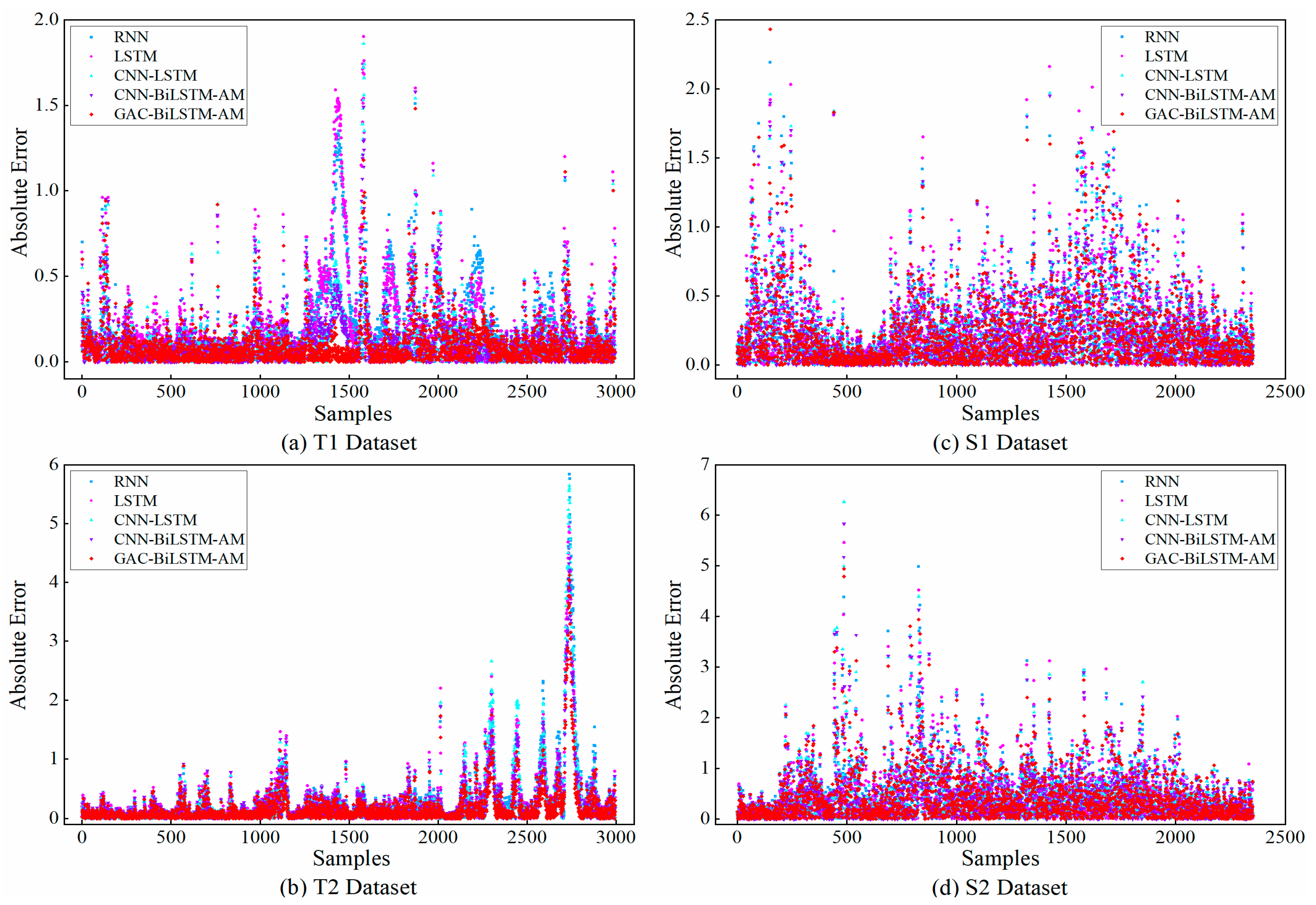
RNN, LSTM, CNN-LSTM, CNN-BiLSTM-AM and GAC-BiLSTM-AM models were built, respectively, to predict the one-step and five-steps-ahead results of the key variables in each public dataset, and the resulting evaluation indexes are shown in

Table 3. Prediction performance evaluation metrics in public datasets.

Dataset	Model	Type	Single Step				Multistep
			MAE	RMSE	R2	SMAPE	MAE	RMSE	R2	SMAPE
T1	RNN	Mean	0.1956	0.3097	0.9906	10.5830	0.5013	0.6798	0.9569	26.7787
	LSTM		0.2029	0.3300	0.9899	11.9854	0.4964	0.6628	0.9594	26.5938
	CNN-LSTM		0.1413	0.2224	0.9954	10.6319	0.5445	0.7333	0.9502	27.5085
	CNN-BiLSTM-AM		0.1467	0.2171	0.9956	10.7290	0.3223	0.4745	0.9791	19.5044
	GAC-BiLSTM-AM		0.1127	0.1694	0.9973	9.3442	0.2889	0.4231	0.9835	17.8501
	RNN	Standard Deviation	0.0445	0.0785	0.0043	0.9546	0.0722	0.0788	0.0097	3.3371
	LSTM		0.0211	0.0355	0.0020	0.4756	0.0343	0.0388	0.0046	0.7805
	CNN-LSTM		0.0085	0.0235	0.0009	0.6385	0.0457	0.0619	0.0083	0.6608
	CNN-BiLSTM-AM		0.0238	0.0305	0.0012	1.0996	0.0339	0.0453	0.0041	0.6625
	GAC-BiLSTM-AM		0.0083	0.0093	0.0002	0.5550	0.0153	0.0149	0.0011	0.5743
T2	RNN	Mean	0.2628	0.6255	0.9859	9.0843	0.5827	0.9722	0.9664	23.3644
	LSTM		0.2704	0.5911	0.9876	10.0469	0.6276	1.0324	0.9623	24.5254
	CNN-LSTM		0.2841	0.6507	0.9849	10.3113	0.6041	0.9879	0.9655	24.1981
	CNN-BiLSTM-AM		0.2547	0.5206	0.9903	10.0396	0.4431	0.7741	0.9787	18.0829
	GAC-BiLSTM-AM		0.1919	0.4189	0.9938	7.9341	0.4018	0.7102	0.9821	16.9569
	RNN	Standard Deviation	0.0227	0.0882	0.0040	0.4293	0.0361	0.0875	0.0062	0.5551
	LSTM		0.0202	0.0512	0.0021	0.5306	0.0366	0.0649	0.0047	0.8959
	CNN-LSTM		0.0258	0.0686	0.0032	0.5829	0.0304	0.0689	0.0047	0.6880
	CNN-BiLSTM-AM		0.0266	0.0578	0.0021	0.7765	0.0338	0.0738	0.0040	0.6456
	GAC-BiLSTM-AM		0.0079	0.0201	0.0005	0.3339	0.0173	0.0434	0.0021	0.5805
S1	RNN	Mean	0.2450	0.3621	0.9894	1.7781	0.4969	0.7104	0.9595	3.6177
	LSTM		0.2719	0.3974	0.9873	1.9873	0.5019	0.7153	0.9590	3.6602
	CNN-LSTM		0.2489	0.3668	0.9891	1.8164	0.4948	0.7049	0.9601	3.6159
	CNN-BiLSTM-AM		0.2483	0.3679	0.9891	1.8061	0.3739	0.5531	0.9754	2.7204
	GAC-BiLSTM-AM		0.2277	0.3418	0.9906	1.6522	0.3613	0.5448	0.9762	2.6292
	RNN	Standard Deviation	0.0035	0.0043	0.0002	0.0286	0.0036	0.0032	0.0003	0.0328
	LSTM		0.0039	0.0047	0.0003	0.0323	0.0022	0.0010	0.0001	0.0204
	CNN-LSTM		0.0064	0.0082	0.0004	0.0468	0.0061	0.0051	0.0005	0.0550
	CNN-BiLSTM-AM		0.0082	0.0100	0.0005	0.0652	0.0038	0.0042	0.0003	0.0294
	GAC-BiLSTM-AM		0.0043	0.0047	0.0002	0.0336	0.0052	0.0056	0.0004	0.0468
S2	RNN	Mean	0.4813	0.7069	0.9906	2.3613	0.8970	1.2798	0.9688	4.3270
	LSTM		0.4651	0.6909	0.9910	2.2590	0.9021	1.2852	0.9685	4.3780
	CNN-LSTM		0.4579	0.7005	0.9908	2.2419	1.0353	1.4535	0.9597	4.8998
	CNN-BiLSTM-AM		0.4505	0.6852	0.9912	2.2039	0.8659	1.2646	0.9694	4.0737
	GAC-BiLSTM-AM		0.4316	0.6521	0.9920	2.1065	0.8560	1.2071	0.9721	4.0296
	RNN	Standard Deviation	0.0695	0.0591	0.0017	0.5007	0.0162	0.0095	0.0004	0.1079
	LSTM		0.0067	0.0118	0.0003	0.0319	0.0098	0.0111	0.0005	0.0601
	CNN-LSTM		0.0125	0.0216	0.0005	0.0674	0.0550	0.0684	0.0037	0.2193
	CNN-BiLSTM-AM		0.0125	0.0291	0.0007	0.0655	0.0691	0.0948	0.0048	0.2721
	GAC-BiLSTM-AM		0.0094	0.0182	0.0004	0.0575	0.0623	0.0759	0.0035	0.2471
ETTh1	RNN	Mean	0.7854	1.1449	0.8868	4.6069	1.8070	2.3459	0.5267	10.3818
	LSTM		0.9797	1.4075	0.8279	5.6366	2.0466	2.6310	0.4041	11.7075
	CNN-LSTM		0.8204	1.1748	0.8804	4.7396	1.9522	2.5140	0.4556	10.9902
	CNN-BiLSTM-AM		0.8206	1.1688	0.8817	4.7479	1.4049	1.9210	0.6824	8.0583
	GAC-BiLSTM-AM		0.7818	1.1214	0.8913	4.5674	1.3550	1.8658	0.7004	7.8174
	RNN	Standard Deviation	0.0155	0.0136	0.0027	0.0898	0.0389	0.0454	0.0186	0.2209
	LSTM		0.0608	0.1123	0.0279	0.3217	0.0690	0.1011	0.0464	0.4262
	CNN-LSTM		0.0475	0.0749	0.0157	0.2326	0.0934	0.1142	0.0493	0.4185
	CNN-BiLSTM-AM		0.0470	0.0631	0.0129	0.2446	0.0475	0.0639	0.0212	0.2257
	GAC-BiLSTM-AM		0.0405	0.0416	0.0081	0.2057	0.0474	0.0569	0.0180	0.2427

.

As can be seen from Table 3, on average, the prediction abilities of RNN and LSTM were very close to each other and did not present a situation where a certain model had an absolute advantage. However, the prediction accuracy of CNN-LSTM was improved compared to LSTM in some tasks, indicating that LSTM could handle complex patterns in the data more efficiently with the help of features extracted from CNN, but its generalization ability and stability were relatively weak. To address this, the CNN-BiLSTM-AM model was further optimized to enhance its versatility. As indicated in the table, the mean indexes of CNN-BiLSTM-AM were better than those of the other three comparative methods in most cases. 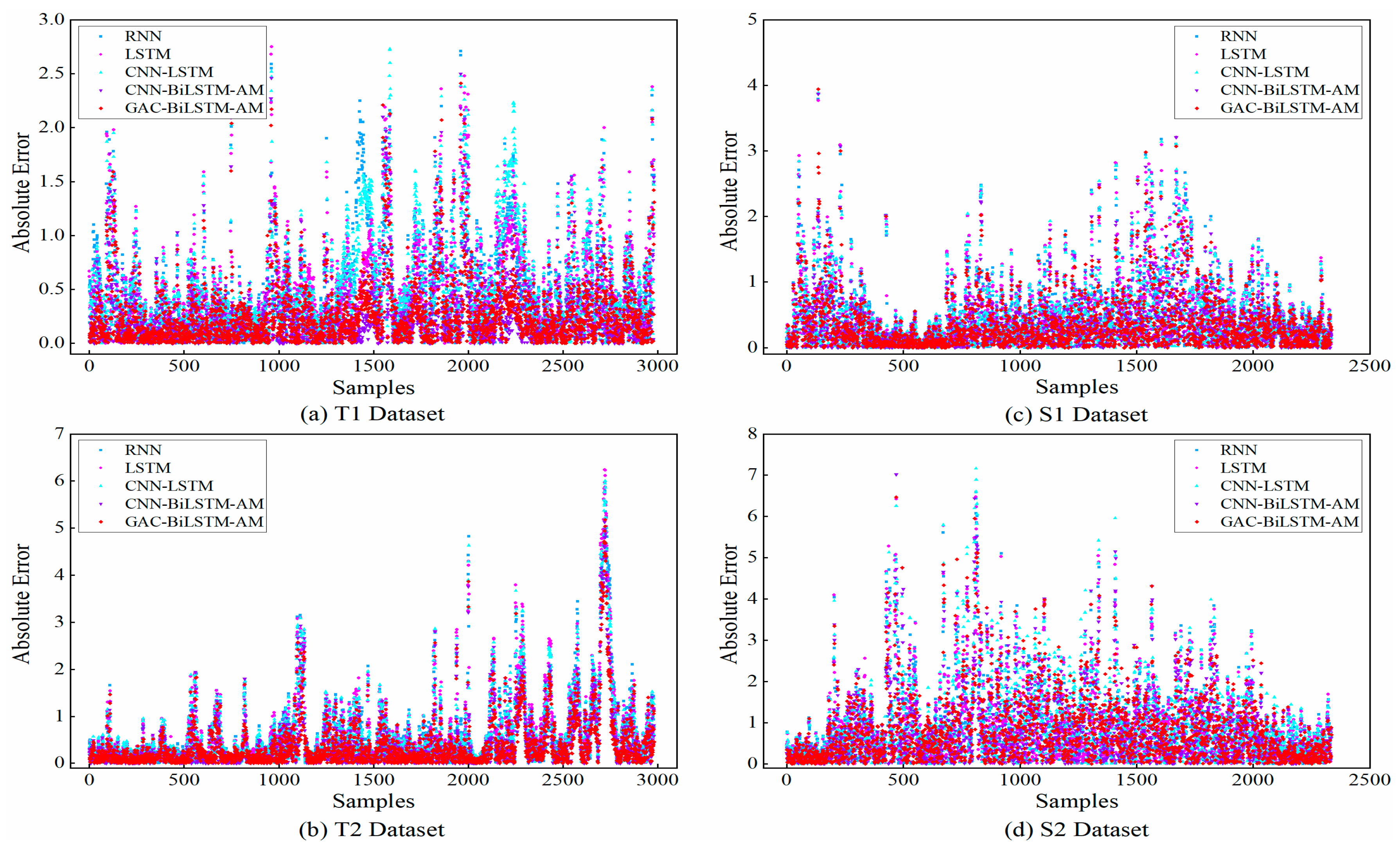Our model, when compared to CNN-BiLSTM-AM, achieved a maximum additional improvement in R² of 0.018, with corresponding reductions in MAE, RMSE, and SMAPE by 0.0499, 0.0552, and 0.2409, respectively, demonstrating superior predictive performance. When shifting from single-step prediction to multi-step prediction, although the prediction accuracy and stability of all models generally decrease, our model exhibits a relatively low decrease, which further validates its advantages in dealing with the long-term dependencies of time series data. The scatter plots of the absolute prediction errors of the models in the single-step and multi-step prediction tasks for the T1, T2, S1, and S2 datasets are shown in Figure 5 and Figure 6, respectively. As shown in these figures, the prediction values of our model were closest to the real values. The comparison of the absolute prediction error curves for the two models with the best performance in single-step and multi-step forecasting tasks on the ETTh1 dataset is shown in Figure 7. This figure shows that the prediction error of our model was still the lowest in most cases, which is consistent with the results in Table 3.

Overall, the GAC-BiLSTM-AM model achieves the highest R² and the lowest MAE, RMSE, and SMAPE across all public datasets, and it also demonstrates excellent stability in most cases. This fully showcases the superior performance of the GAC-BiLSTM-AM model.

3.3. Fluent Simulation Data

3.3.1. Dataset Introduction and Model Parameter Settings

Fluent simulation data are a cross-section dataset obtained by building a furnace combustion model, a turbulence model, and an ethylene cracking reaction model to simulate the process of ethylene cracking on fluent [32] simulation software, respectively. The dataset has a total of 50,025 pieces of data and 18 features, among which, t_ p represents the furnace tube temperature, which is the prediction target of this experiment, and its first 10,000 pieces of data are taken to form the F1 dataset in the experiment, and the ratio of the training and test data is set to 7:3. The model parameters of GAC-BiLSTM-AM are shown in

Table 4. Parameters of the GAC-BiLSTM-AM model in simulated data.

Parameters	Value
	Single Step	Multistep
Single-layer convolution filters	77	77
Single-layer convolution kernel size	1	1
Three-layer convolution filters	19/38/77	19/38/77
Three-layer convolution kernel size	1	1
Full connection layer output size	77	77
First dropout rate	0	0
Number of hidden units in BiLSTM layer	77	77
Second dropout rate	0.000325415686	0.000325415686
Initial value	0.25	10.5
Decrement	0.005	0.2
Weight update interval value	11	11
Threshold	0.15	4.5

.

3.3.2. Result Analysis

The GAC-BiLSTM-AM model is compared and analyzed with the RNN, LSTM, CNN-LSTM, and CNN-BiLSTM-AM models, and the evaluation indexes obtained are shown in

Table 5. Performance evaluation metrics for furnace tube temperature prediction.

Model	Type	Single Step				Multistep
		MAE	RMSE	R2	SMAPE	MAE	RMSE	R2	SMAPE
RNN	Mean	1.8629	3.0479	0.9941	0.2155	2.5727	5.1194	0.9835	0.2968
LSTM		1.9986	3.3029	0.9931	0.2303	2.3710	5.0612	0.9838	0.2730
CNN-LSTM		1.9767	3.2648	0.9932	0.2279	2.6478	5.2455	0.9825	0.3044
CNN-BiLSTM-AM		2.0575	3.3136	0.9930	0.2368	2.1849	3.5638	0.9920	0.2520
GAC-BiLSTM-AM		1.8135	3.0100	0.9943	0.2094	2.1255	3.5133	0.9922	0.2448
RNN	Standard Deviation	0.0327	0.0361	0.0001	0.0037	0.0498	0.0284	0.0001	0.0055
LSTM		0.1061	0.1461	0.0006	0.0118	0.1135	0.1643	0.0010	0.0124
CNN-LSTM		0.0699	0.0959	0.0003	0.0081	0.5341	0.4556	0.0033	0.0593
CNN-BiLSTM-AM		0.3355	0.3911	0.0018	0.0371	0.0615	0.0908	0.0004	0.0069
GAC-BiLSTM-AM		0.0468	0.0671	0.0002	0.0052	0.0349	0.1046	0.0004	0.0039

.

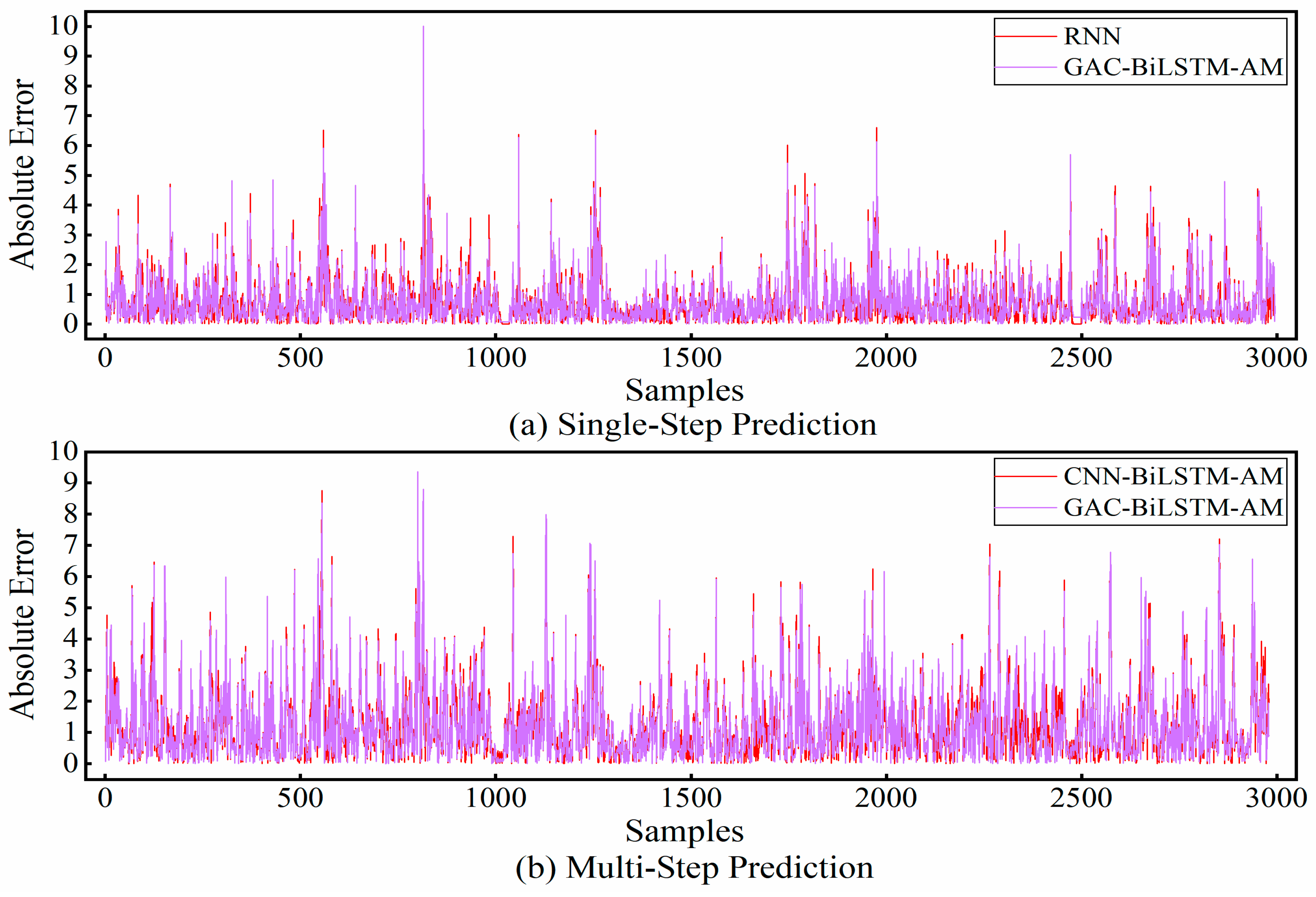
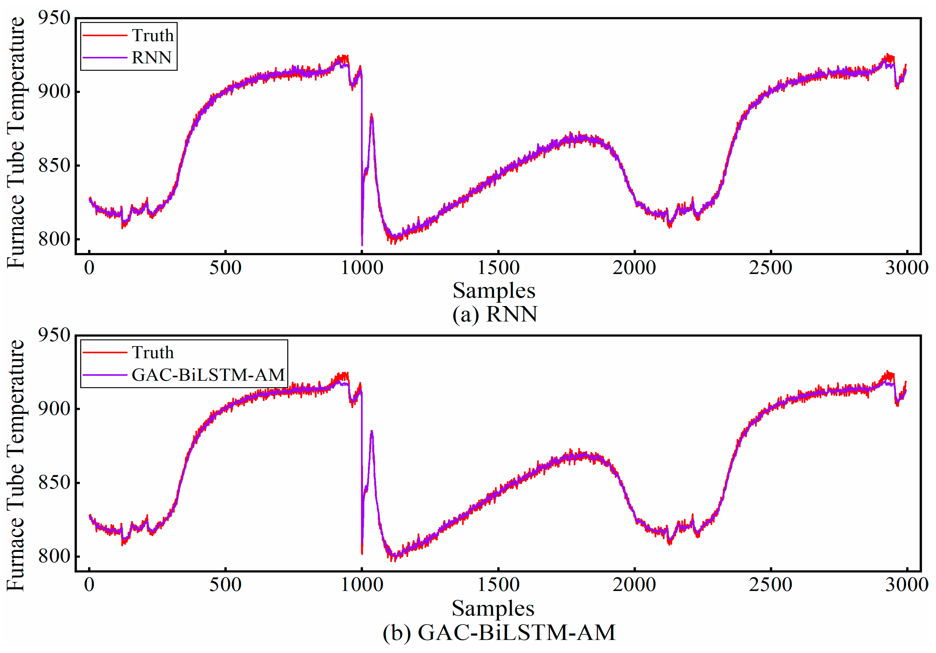
As shown in Table 5, the CNN-BiLSTM-AM model exhibits the worst prediction performance among the five models in single-step forecasting. By observing the standard deviation of the results from ten runs, it is found that the highest value is attributed to the CNN-BiLSTM-AM, indicating poor stability in this model, which leads to less-than-ideal prediction outcomes. In contrast, both the RNN and GAC-BiLSTM-AM models demonstrate superior prediction performance. A comparison of their single-step forecasting results is presented in Figure 8. From the figure, it can be observed that in non-transitional regions, the GAC-BiLSTM-AM model has a smaller deviation between the predicted values and the actual values, which is the reason for its higher accuracy.

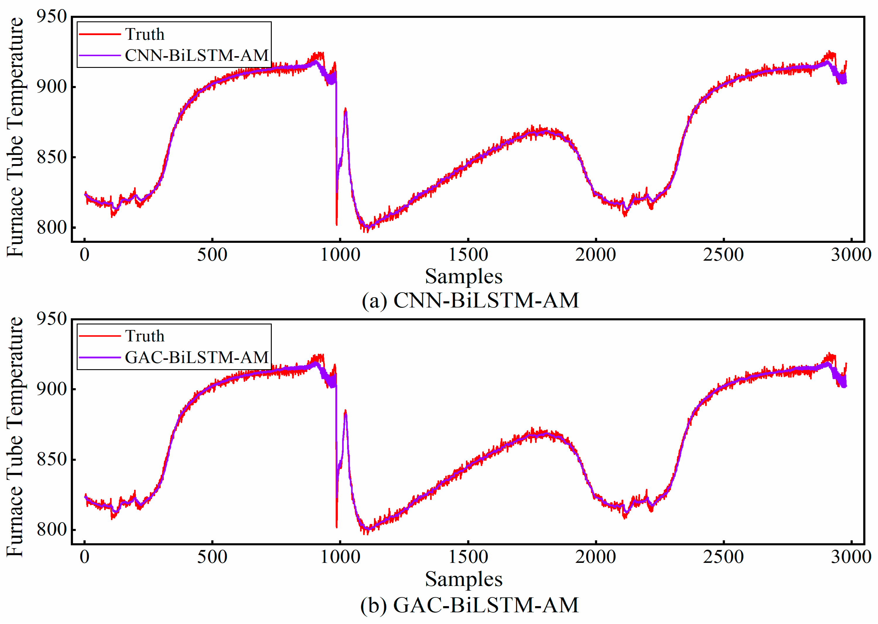
With multi-step prediction, the prediction accuracy of RNN decreases more significantly compared to single-step prediction, and its MAE, RMSE, and SMAPE are improved by 38.1%, 67.96%, and 37.72%, respectively, and R² is reduced by 1.06%. This situation arises because RNN gradually encounters the long sequence dependence issue as the input step size increases. In contrast, CNN-BiLSTM-AM and GAC-BiLSTM-AM have demonstrated better performance than RNN. Primarily, these model alleviates long-sequence dependence and information overload issues. This is achieved by leveraging the synergy between the attention mechanism and the information stored in the cell state. A comparison of the two models’ multi-step prediction results is depicted in Figure 9. As seen in the figure, the latter model exhibits a superior fitting effect, which is mainly attributable to GAC-BiLSTM-AM’s ability to perform more comprehensive information analysis, thereby ensuring the model achieves higher prediction accuracy.

The above results show that our model is more applicable in the prediction task, and it possesses higher robustness and stronger generalization.

3.4. Parameter Comparison and Ablation Analysis

In the comparison stage above, the structural parameters used in our model are not the optimal parameters for all tasks. In order to understand the optimal performance of the model in each dataset and, at the same time, grasp the true effect of our model when using the comparison method parameters, the following parametric contrast experiments were conducted and the results obtained are shown in

Table 6. Performance evaluation metrics for different parameter predictions.

Dataset	Category	Single Step				Multistep
		MAE	RMSE	R2	SMAPE	MAE	RMSE	R2	SMAPE
F1	1 *	1.8128	2.9891	0.9943	0.2094	2.1291	3.5361	0.9921	0.2454
	1 ′	1.8378	3.0173	0.9942	0.2122	2.1397	3.5527	0.9920	0.2466
	2 ′	1.8137	3.0074	0.9943	0.2094	2.1187	3.5094	0.9922	0.2441
	3 ′	1.7362	2.9098	0.9946	0.2008	2.0577	3.3799	0.9928	0.2372
T1	1 *	0.1205	0.1846	0.9968	9.7427	0.2796	0.4234	0.9835	17.3301
	1 ′	0.1205	0.1847	0.9968	9.7421	0.2784	0.4222	0.9836	17.5117
	2 ′	0.1106	0.1690	0.9973	9.3151	0.2881	0.4271	0.9832	17.8237
	3 ′	0.1106	0.1690	0.9973	9.3151	0.2791	0.4151	0.9841	17.4587
T2	1 *	0.2132	0.4610	0.9924	8.5050	0.4127	0.7214	0.9816	17.2423
	1 ′	0.2137	0.4619	0.9924	8.5023	0.4072	0.7119	0.9820	17.1746
	2 ′	0.1964	0.4280	0.9935	8.0153	0.4055	0.7100	0.9822	17.0832
	3 ′	0.1908	0.4154	0.9939	7.9188	0.3958	0.6954	0.9829	16.9032
S1	1 *	0.2308	0.3444	0.9904	1.6792	0.3676	0.5501	0.9757	2.6772
	1 ′	0.2302	0.3433	0.9905	1.6764	0.3695	0.5498	0.9757	2.6969
	2 ′	0.2284	0.3422	0.9905	1.6582	0.3620	0.5459	0.9761	2.6338
	3 ′	0.2246	0.3370	0.9908	1.6317	0.3579	0.5401	0.9766	2.6062
S2	1 *	0.4284	0.6420	0.9922	2.0901	0.8733	1.2373	0.9707	4.0851
	1 ′	0.4261	0.6395	0.9923	2.0853	0.8737	1.2333	0.9709	4.0953
	2 ′	0.4322	0.6537	0.9920	2.1104	0.8142	1.1656	0.9740	3.8709
	3 ′	0.4203	0.6246	0.9927	2.0465	0.7848	1.1381	0.9752	3.7156
ETTh1	1 *	0.7770	1.1159	0.8923	4.5366	1.3612	1.8757	0.6971	7.8015
	1 ′	0.7775	1.1168	0.8921	4.5386	1.3738	1.8928	0.6915	7.8555
	2 ′	0.7836	1.1240	0.8908	4.5746	1.3585	1.8743	0.6975	7.8285
	3 ′	0.7622	1.0976	0.8959	4.4714	1.3260	1.8293	0.7121	7.6557

. In the table, 1 indicates the use of the same parameters as the comparison method, 2 indicates the use of the experimental parameters above, 3 indicates the use of the respective optimized structural parameters, and * indicates that the graphics card model used is the T400 (all experiments mentioned above were conducted using the T400), and ′ indicates that the graphics card model is the A10.

By comparing the results in the table with the above, we find that the performance of our model remains optimal in most of the datasets when using the same parameters, which further confirms the superiority of our model’s performance. Meanwhile, from Table 6, it can be seen that the structural parameters obtained from the optimization are more effective in improving the multi-step prediction accuracy. If the model uses the respective optimization structural parameters in all of the above datasets, the R² value can be further increased by a maximum of 0.0146 over the existing optimal results. The MAE, RMSE, and SMAPE, correspondingly, decrease by 0.0325, 0.045, and 0.1728, respectively, and prediction errors are further minimized. This also confirms the effectiveness of the optimization algorithm used.

Our model is an improvement on the CNN-BiLSTM-AM model. Specifically, we made the following three changes: 1) added a mistake correction mechanism; 2) optimized the feature extraction module; and 3) added the Adaboost algorithm and linear regression model. To understand the impact of these improvements on the final results, we conducted ablation analysis using the T2 and S2 datasets. The reason for choosing these two datasets is that the T2 dataset retains more features after the feature selection, while the S2 dataset retains fewer features after the feature selection. The number of features input into the network for both basically represents the current feature status of all the data, making the experimental results more persuasive. In the experiment, we only changed the structure of the model, and the results are shown in

Table 7. Ablation results.

Dataset	Category	Single Step				Multistep
		MAE	RMSE	R2	SMAPE	MAE	RMSE	R2	SMAPE
T2	a	0.1908	0.4154	0.9939	7.9188	0.3958	0.6954	0.9829	16.9032
	b	0.1968	0.4266	0.9935	8.0349	0.4031	0.7079	0.9823	17.0896
	c	0.2419	0.5085	0.9908	9.6695	0.4462	0.7864	0.9782	18.1005
	d	0.2491	0.5141	0.9906	9.8501	0.4585	0.8033	0.9771	18.4797
S2	a	0.4203	0.6246	0.9927	2.0465	0.7848	1.1381	0.9752	3.7156
	b	0.4237	0.6331	0.9925	2.0668	0.8041	1.1674	0.9738	3.8048
	c	0.4549	0.7044	0.9907	2.2351	0.7990	1.1765	0.9735	3.7665
	d	0.4568	0.7016	0.9907	2.2480	0.8323	1.2111	0.9720	3.9080

. In the table, a represents the current model, b has the error correction mechanism removed, c replaces the feature extraction module on the basis of b, and d is the CNN-BiLSTM-AM model. By comparing the results in the table, we can draw the following conclusions:

(1)

During the iterative optimization of model parameters, the mistake correction mechanism can dynamically adjust the weights of samples, effectively correcting the model’s focus and promoting a more balanced learning process, which, in turn, enhances the model’s generalization performance.

(2)

The dual-channel convolutional neural network excels in processing complex data with rich features, and the deep semantic information it extracts markedly improves the model’s comprehension capabilities.

(3)

By integrating the Adaboost algorithm and linear regression model and synthesizing the different focuses of these two base learners, the model’s ability to analyze information comprehensively is enhanced.

3.5. Real Industrial Data

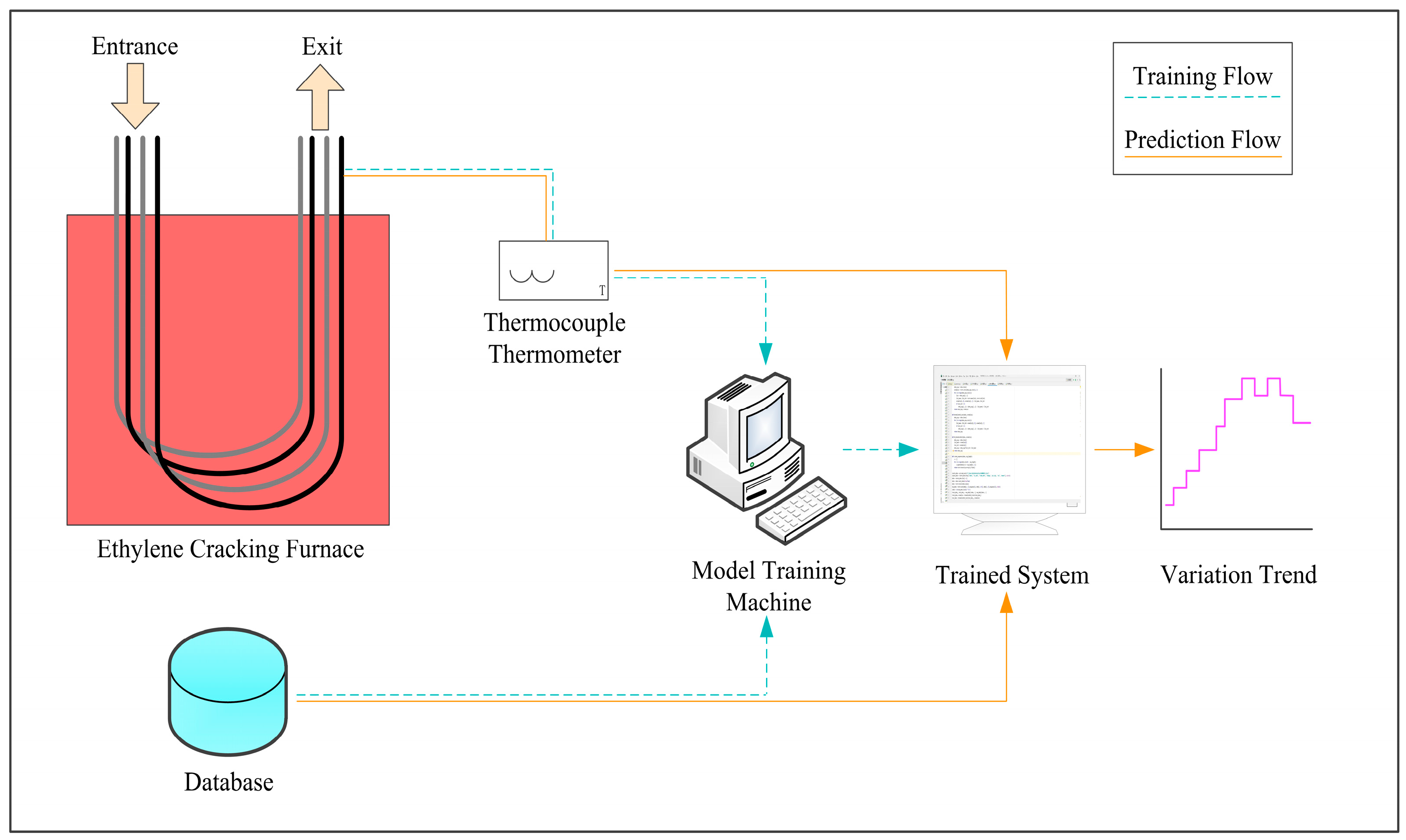
When the cracking outlet temperature (COT) is too high, it accelerates the coking rate on the inner wall of the cracking furnace tubes. When the temperature is too low, it affects the cracking efficiency [33]. Therefore, in the ethylene production process, regulating the COT is critical. The current real-time monitoring and control methods require a certain amount of time to adjust the temperature, subject to lag. If the future temperature trend can be known in advance, measures can be taken as early as possible to further optimize the production process. Therefore, we apply the methodology of this paper to COT prediction. It is worth mentioning that our method is also suitable for solving complex industrial prediction problems that need to consider the spatial distribution, time-series dynamics, and multivariate interactions at the same time—for example, the prediction of energy loads and the prediction of equipment failures. The real data used are sourced from the 1# ethylene cracking unit of a large state-owned petrochemical company in China. 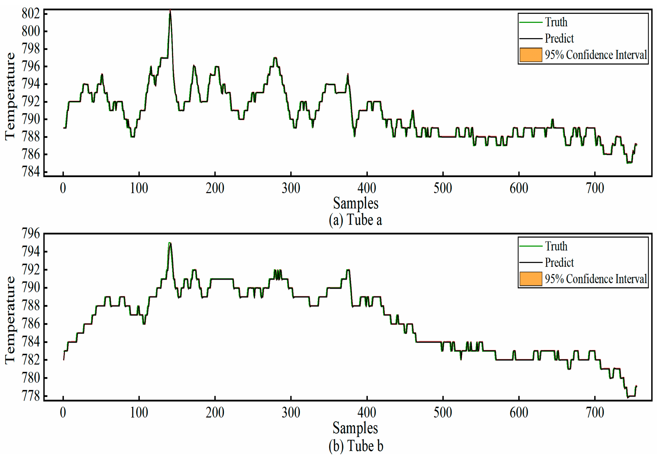The unit consists of 11 USC-type cracking furnaces, numbered from H-110 to H-120 [34]. We randomly select two furnace tubes from the H-115 cracking furnace as the validation objects, named tube a and tube b, respectively. Then, we collect 5760 pieces of data as the experimental data for single-step prediction. Of these, the first 5000 pieces of data are used as training data, and the remaining 760 pieces of data are used as test data. The parameters of the GAC-BiLSTM-AM model are set as shown in

Table 8. Parameters of the GAC-BiLSTM-AM model in real data.

Parameters	Value
	Single Step	Multistep
Single-layer convolution filters	58	54
Single-layer convolution kernel size	1	1
Three-layer convolution filters	14/29/58	14/27/54
Three-layer convolution kernel size	1	1
Full connection layer output size	58	54
First dropout rate	0	0.000126706879
Number of hidden units in BiLSTM layer	58	54
Second dropout rate	0.033348504	0.00320840064
Initial value	0.25	0.25
Decrement	0.005	0.005
Weight update interval value	6	6
Threshold	0.15	0.15

. The overall framework of the prediction system is shown in Figure 10.

The experimental results show that for tube a, the MAE is 0.2629, the RMSE is 0.4895, the R² is 0.9702, and the SMAPE is 0.0332; for tube b, the MAE is 0.1761, the RMSE is 0.3978, the R² is 0.9882, and the SMAPE is 0.0223. The required running times for each are 11.53 s and 10.96 s, respectively. The prediction results are presented in Figure 11. As can be seen from the figure, the model’s predicted values closely match the actual values, with the maximum prediction error being within 2 °C. This can provide a reliable reference for the relevant staff to grasp the changes in temperature in advance. Furthermore, the time expenditure also satisfies the requirements of practical applications. Consequently, applying our method to predict the cracking outlet temperature in ethylene cracking furnaces holds significant practical relevance.

4. Conclusions

To address the common problem of insufficient generalization capability in prediction models, we have proposed a novel GAC-BiLSTM-AM prediction method. This method, by means of dual-channel feature extraction and dynamic attention modification, further improves the generalization ability of the composite model and strengthens its robustness in prediction tasks. Additionally, to overcome the limitations of empirical parameter setting, we utilize the gold rush optimizer for the adaptive optimization of parameters. By establishing a multi-objective optimization mechanism to ensure the rationalization of structural parameters. Experimental results from multiple prediction tasks indicate that our method exhibits outstanding generalization performance. In the application of predicting the cracking furnace outlet temperature, the prediction error consistently remains within ±2 °C, fully capable of providing reliable technical support for actual industrial production. However, since our method is based on the integration of composite models, it has, to some extent, increased the time complexity of the model. How to simplify the model while maintaining the prediction accuracy will be a key research direction for the future.