Numerical Simulation of Non-Isothermal Two-Phase Flow in Oil Reservoirs, Including Heated Fluid Injection, Dispersion Effects, and Temperature-Dependent Relative Permeabilities

Abstract

This study addresses the numerical simulation of non-isothermal two-phase water-oil flow in oil reservoirs. The problem of heavy oil recovery by reservoir heating (via heated fluid injection) is investigated, aiming to reduce oil viscosity and increase its mobility. The governing equations are formulated in terms of non-wetting phase pressure (oil), wetting phase saturation (water), and reservoir average temperature, without assuming local thermal equilibrium. Temperature-dependent relative permeabilities are considered. The Finite Volume Method is employed, and the resulting algebraic equations are linearized using the Picard method. The linearized discretized equations are solved sequentially for pressure, saturation, and average temperature, utilizing the Preconditioned Conjugate Gradient (pressure and average temperature) and Preconditioned Stabilized Biconjugate Gradient Method (saturation). After validating the numerical results, a sensitivity analysis is performed using a reservoir with slab geometry. The results demonstrate the positive impact of reservoir heating on heavy oil recovery.

1. Introduction

Energy generation, the environment, health, and biological systems are areas where porous media flow knowledge is significant. Examples include oil and gas exploitation, fuel cells, batteries, solid mechanics, and cardiovascular systems [1]. Numerical simulation, for instance, finds application in the oil industry, which invests substantial resources to mitigate costs and risks associated with production.

Data about flow patterns can be obtained through experiments using reservoir samples. Alternatively, information can be collected via pressure tests in injection/producing wells and temperature and pressure data analysis. However, these methods are expensive and may be unfeasible when studying multiple production scenarios. For this purpose, numerical simulation becomes a valuable alternative tool [2]. In this context, this study proposes its use to solve non-isothermal two-phase flow using a one-equation model derived without assuming the hypothesis of local thermal equilibrium.

Numerical reservoir simulation requires a prior understanding of several areas of knowledge, such as mathematics, physics, numerical methods, and advanced programming [3], and it is widely used in the oil industry [2]. This is due to the inherent difficulties in accurately obtaining reservoir properties throughout its extension and the complexity of determining flow behavior in situ. Therefore, it serves as an ally when maximizing hydrocarbon recovery is necessary [4,5]. Hydrocarbon production stages can be divided into primary, secondary, and tertiary [6]. In primary production, oil or gas is obtained due to the pressure difference between the reservoir interior and the surface. In secondary production, part of the remaining hydrocarbons is recovered via the injection of an immiscible fluid, available in abundance and at low cost. Finally, chemical, miscible displacement, biological, and thermal methods are employed [7]. All aim to promote higher hydrocarbon mobility, decreasing flow resistance and increasing production [6].

In the case of conventional oils (API gravity greater than 30), production costs are comparatively lower than those associated with heavier oils [8]. However, due to the current depletion of their reserves, special attention has been given to exploring those with API gravity between 5 and 22. As they have higher viscosity, there is higher flow resistance, and production costs are higher [9]. Under these circumstances, the dominant recovery techniques are thermal, non-thermal, or cold and solvent-based [10].

Therefore, an attractive alternative to increase heavy oil recovery is the use of thermal methods [11]. For example, static heaters can be positioned inside the reservoir, resulting in a decrease in viscosity and a consequent increase in fluidity [12].

As with other recovery techniques, numerical simulation can also be used for thermal methods [13]. The most commonly used is steam injection [14], which has the disadvantage of requiring a large amount of available water in addition to the energy cost associated with steam generation. Furthermore, it causes harmful environmental effects due to the means generally used to generate the necessary energy, causing the emission of greenhouse gases [14]. An alternative, in situ combustion, has been applied with relative success in Canada [10].

Electric energy can also be used to heat the reservoir by introducing heating elements that transfer heat to the fluid and the rock [9,15]. Another possibility is electromagnetic heating, enabling localized heating and being able to transfer up to 92% of the generated energy to its surroundings [16]. The number and location of the heating elements can vary to maximize the recovery process.

In the physical-mathematical modeling of porous media flow, compared to isothermal flow, the energy equation must be considered in non-isothermal flow in addition to the continuity and momentum equations. In the literature, one- or two-equation models are commonly used, with the latter being the most suitable when there are significant differences in the order of magnitude of the thermal properties of the fluids and the porous matrix [17]. The one-equation model for single-phase flow [13,18] can be derived with or without assuming the hypothesis of local thermodynamic equilibrium [19]. In the case of the two-equation model [17], separate equations are used to obtain the temperature of the fluid and the rock, and the heat transfer between them is accounted for via a source term [20].

In the most general case, multiphase flow must be considered due to the presence of more than one phase when using advanced recovery techniques. For example, Siavashi et al. [21] simulated the non-isothermal two-phase flow of immiscible fluids in a saturated medium, adopting the hypothesis of local thermal equilibrium, and simulated the injection of heated water via the streamline method. On the other hand, also assuming local thermal equilibrium, Roy et al. [22] studied the non-isothermal, compositional two-phase flow, considering the presence of chemical reactions. Other applications can be found in Lindner et al. [23] and Kumar et al. [24]. The first dealt with cooling by phase change and used a mixing model, considering a multi-component fluid, without considering local thermal equilibrium. The last one addressed the drying process in food via microwaves, in which a fluid flow model in a porous medium with phase change was used.

Although phase changes may occur due to the temperature increase inside the reservoir, they were not considered here. As a preventive measure, the maximum temperature values were monitored to prevent them from occurring. Therefore, the case of a three-phase flow is outside the scope. In this initial work, the problem of injecting a heated fluid into a reservoir with slab geometry will be addressed. Later, the heating problem using static heating wells will be investigated.

This research advances the understanding of non-isothermal two-phase flow in porous media by explicitly considering the interplay of temperature-dependent relative permeabilities and hydrodynamic dispersion. Its innovation also lies in the use of a proposed operator decomposition, enabling the application of Conjugate Gradient (CG) and Biconjugate Gradient Stabilized (BiCGSTAB) methods to solve, in a fully implicit manner, the subsystems for oil pressure (CG), temperature (CG), and water phase saturation (BiCGSTAB). This approach provides novel insights into this area, particularly relevant for enhanced oil recovery.

2. Non-Isothermal Flow in Porous Media

The governing equations that will provide the saturation and average temperature of the reservoir are presented below, along with the specification of how the properties of the fluids and the porous matrix will be calculated.

The following hypotheses were considered in the model used:

• the rock formation is anisotropic in terms of absolute permeability;
• the rock compressibility is small and constant;
• the fluids are Newtonian;
• no chemical reactions occur;
• the flow is laminar at a very low velocity;
• the fluids have a steady chemical composition;
• the flow is non-isothermal, two-phase and three-dimensional;
• the fluids are slightly compressible;
• the thermal conductivities of the rock and fluids are constant;
• and the hypothesis of local thermal equilibrium is not considered.

Each of these assumptions simplifies the simulation model, but also introduces limitations. The anisotropy of rock permeability directly affects the direction and velocity of flow, requiring a model that captures this directional variation. The low compressibility of rock and fluids simplifies density and volume calculations. The Newtonian nature of fluids and the absence of chemical reactions eliminate complexities related to nonlinear behavior and species production or consumption. Low-velocity laminar flow justifies the use of modified Darcy law. The constant chemical composition of fluids and the constant thermal conductivity of rock and fluids reduce the need for complex heat transport and transfer models. The non-isothermal, two-phase, three-dimensional nature of the flow requires the solution of energy and multiphase flow equations. Finally, the disregard of local thermal equilibrium allows modeling situations where the average temperature of the rock and fluids are not the same.

In accordance with the scope of this study, fluid and rock properties are computed as functions of both pressure and temperature, with particular emphasis on the implementation of a model for temperature-dependent relative permeabilities.

It is also important to highlight that this set of hypotheses defines a specific scope wherein the flow maintains a two-phase state under the prescribed conditions, excluding water evaporation or gas dissolution from the liquid phases.

For two-phase flow in porous media, the mass balance yields [3]

$${\displaystyle \frac{\partial }{\partial t}}\left(\varphi {\rho }_{\alpha }{S}_{\alpha }\right)+\nabla .\left({\rho }_{\alpha }{\mathbf{v}}_{\alpha }\right)-q_{m\alpha }=0,$$

(1)

where $\varphi$ is the porosity, $\rho$ is the density, $\mathbf{v}$ is the superficial velocity, S is the saturation, $q_m$ is the source term, and the subscript $\alpha$ indicates the phase in question. Furthermore,

$$\varphi ={\varphi }^0\left[1+c_{\varphi }\left(p_o-p^0\right)-c_{\varphi T}\left(T-T^0\right)\right],$$

(2)

where ${\varphi }^0$ is the reference porosity, determined at the reference pressure ($p^0$) and temperature ($T^0$), $c_{\varphi }$ is the rock compressibility coefficient, $c_{\varphi T}$ represents the rock thermal expansivity coefficient, $p_o$ is the pressure of the non-wetting phase (oil) and T is the mean reservoir temperature (to be defined later) [3].

Regarding density [3], we employ

$${\rho }_{\alpha }={\rho }_{\alpha }^0\left[1+c_{\alpha }\left(p_{\alpha }-p^0\right)-c_{\alpha T}\left(T-T^0\right)\right],$$

(3)

where ${\rho }_{\alpha }^0$ is the density of the phase $\alpha$ under reference conditions, $c_{\alpha }$ is the fluid compressibility coefficient, and $c_{\alpha T}$ is the thermal expansion coefficient of the phase $\alpha$.

Although viscosity varies depending on pressure and temperature, only its variation with temperature will be considered [13],

$${\mu }_n=a_{n}exp\left({\displaystyle \frac{b_n}{T-T_{ref}}}\right),$$

(4)

where $a_n$ and $b_n$ are constants determined for a given type of oil, $T_{ref}$ is the reference temperature for calculating viscosity, and it is a correlation specifically developed for heavy oils. The water viscosity is considered constant.

In two-phase flow, Darcy’s classical law must be modified by introducing the relative permeability $k_{r\alpha }$ [3],

$${\mathbf{v}}_{\alpha }=-{\displaystyle \frac{k_{r\alpha }}{{\mu }_{\alpha }}}\mathbf{k}\left(\nabla p_{\alpha }-{\gamma }_{\alpha }\nabla Z\right),$$

(5)

where $k_{r\alpha }$ is the relative permeability of $\alpha$ phase, ${\mathsf{\mu }}_{\alpha }$ is the viscosity, $\mathbf{k}$ is the absolute permeability tensor (diagonal), $p_{\alpha }$ is the pressure, $gamm{a}_{\alpha }={\rho }_{\alpha }g$, where g is the magnitude of the acceleration due to gravity, and Z is the depth.

Since this is a non-isothermal flow, a model that takes into account the variation of relative permeability as a function of temperature is used [25]:

$$k_{rw}=exp\left[-0.08832T+15.38ln\left(T\right)-64.87\right]{\left[{\displaystyle \frac{S_w-2.673·{10}^{-4}T-0.0382}{1-2.673·{10}^{-4}T+0.1036ln\left(T\right)-0.7623}}\right]}^{A_1}$$

(6)

for the wetting phase (water), where $A_1=-\mathrm{5,578}·{10}^{-3}T+\mathrm{2,995}$ and, for the non-wetting phase,

$$k_{rn}=\left[0.4947ln\left(T\right)-1.6666\right]{\left[1-{\displaystyle \frac{S_w-2.673·{10}^{-4}T-0.0382}{1-2.673·{10}^{-4}\left(T\right)+0.1036ln\left(T\right)-0.7623}}\right]}^{A_2},$$

(7)

where $A_2=-9.885·{10}^{-4}T+1.349$, $S_w$ is the saturation of the wetting phase, and the temperature T should be given in °C. These correlations are valid for temperatures ranging from 70 to 220 degrees Celsius.

Combining Equations (1) and (5),

$$\nabla ·\left[{\displaystyle \frac{k_{ro}}{{\mu }_o{B}_o}}\mathbf{k}\left(\nabla p_o-{\gamma }_o\nabla Z\right)\right]={\displaystyle \frac{\partial }{\partial t}}\left[{\displaystyle \frac{\varphi S_o}{B_o}}\right]-q_{s{c}_o},$$

(8)

$$\nabla ·\left[{\displaystyle \frac{k_{rw}}{{\mu }_w{B}_w}}\mathbf{k}\left(\nabla p_w-{\gamma }_w\nabla Z\right)\right]={\displaystyle \frac{\partial }{\partial t}}\left[{\displaystyle \frac{\varphi S_w}{B_w}}\right]-q_{s{c}_w},$$

(9)

where $B_{\alpha }={\rho }_{sc\alpha }/{\rho }_{\alpha }$ is the formation-volume factor, $q_{s{c}_w}=q_{mw}/{\rho }_{s{c}_w}$ and $q_{s{c}_o}=q_{mo}/{\rho }_{s{c}_o}$, being ${\rho }_{s{c}_w}$ and ${\rho }_{s{c}_o}$ the densities at standard (constant) conditions of the wetting phase (water), and of the non-wetting phase (oil), respectively.

The reservoir is saturated

$$S_w+S_o=1$$

(10)

and the effects of capillary pressure,

$$p_c=p_o-p_w,$$

(11)

are accounted for [26]

$$p_c\left(S_w\right)=p_{c_{max}}{\left({\displaystyle \frac{1-S_w-S_{ro}}{1-S_{iw}-S_{ro}}}\right)}^{epc},$$

(12)

where $p_{c_{max}}$ is the maximum capillary pressure, the exponent $epc$ must be provided, $S_{iw}$ is the irreducible water saturation, and $S_{ro}$ is the residual oil saturation.

Therefore, substituting Equations (10) and (11) into Equations (8) and (9) yields the two governing equations:

$$\nabla ·\left[{\displaystyle \frac{k_{ro}}{{\mu }_o{B}_o}}\mathbf{k}\left(\nabla p_o-{\gamma }_o\nabla Z\right)\right]={\displaystyle \frac{\partial }{\partial t}}\left[{\displaystyle \frac{\varphi \left(1-S_w\right)}{B_o}}\right]-q_{s{c}_o},$$

(13)

$$\nabla ·\left[{\displaystyle \frac{k_{rw}}{{\mu }_w{B}_w}}\mathbf{k}\left(\nabla p_o-\nabla p_c-{\gamma }_w\nabla Z\right)\right]={\displaystyle \frac{\partial }{\partial t}}\left({\displaystyle \frac{\varphi S_w}{B_w}}\right)-q_{s{c}_w}.$$

(14)

As previously stated, it is common to use the assumption of local thermal equilibrium (equality of volume average temperatures of fluids and porous matrix) [22,27]. However, in some situations, it may be inappropriate [28]. As alternatives, the one-equation model without adopting such an assumption [19], or the two-equation model [17] or three-equations, with phase change [28] or without phase change [29] are available. Here, the one-equation model (without local thermal equilibrium) is employed, whose dependent variable is the volume average reservoir temperature (weighted average of the phase and rock temperatures), and the thermal heating is modeled via source terms [13].

For constant heat capacities, the macroscopic equation governing heat transfer is [30]:

$$\begin{array}{ccc}\hfill {\displaystyle \frac{\partial }{\partial t}}\left[\left(\rho c_p\right)T\right]& -& \nabla ·\left[{\rho }_o{h}_o{\displaystyle \frac{k_{ro}}{{\mu }_o}}\mathbf{k}\left(\nabla p_o-{\gamma }_o\nabla Z\right)\right]-\nabla ·\left[{\rho }_w{h}_w{\displaystyle \frac{k_{rw}}{{\mu }_w}}\mathbf{k}\left(\nabla p_o-\nabla p_c-{\gamma }_w{\nabla }_{w}Z\right)\right]\hfill \\ \hfill & =& \nabla ·(\mathbf{K}\nabla T)+{\displaystyle \frac{q_H}{V_b}}+{\displaystyle \frac{{\rho }_o{h}_o{q}_{s{c}_o}}{V_b}}+{\displaystyle \frac{{\rho }_w{h}_w{q}_{s{c}_w}}{V_b}},\hfill \end{array}$$

(15)

where $\mathbf{K}$ represents the effective thermal dispersion tensor, $h_o$ and $h_w$ are the enthalpies of oil and water, $q_H$ represents a volumetric thermal source (when there are heating wells), $V_b$ is the total volume, and $q_{s{c}_o}$ and $q_{s{c}_w}$ represent the volumetric mass flow rates when there are injection/producing wells.

The average temperature of the porous medium, considering both phases and the rock, is given by [30]:

$$\left(\rho c_p\right)T=\varphi \left(1-S_w\right){\left(\rho c_p\right)}_o{T}_o+\varphi S_w{\left(\rho c_p\right)}_w{T}_w+\left(1-\varphi \right){\left(\rho c_p\right)}_r{T}_r,$$

(16)

where ${c_p}_o$, ${c_p}_w$, $T_o$, and $T_w$ are respectively the specific heat and temperatures of the oil and water, and T represents the average reservoir temperature. Furthermore [30],

$$\left(\rho c_p\right)=\varphi \left(1-S_w\right){\left(\rho c_p\right)}_o+\varphi S_w{\left(\rho c_p\right)}_w+\left(1-\varphi \right){\left(\rho c_p\right)}_r$$

(17)

represents the average heat capacity.

The enthalpies of the fluids are calculated knowing the average temperature of the reservoir [13]:

$$h_o={c_p}_{o}T,h_w={c_p}_{w}T.$$

(18)

For example, after applying the Method of Volume Averaging [31] to the energy balance equation, the appearance of the effective thermal dispersion tensor in the macroscopic equation describing energy transfer at the laboratory scale is observed [19,32]. It contains the contribution of three terms related to thermal conduction, tortuosity, and hydrodynamic dispersion and, in the case of two-phase flow,

$$\mathbf{K}=\left[\varphi \left(1-S_w\right){\kappa }_o+\varphi S_w{\kappa }_w+\left(1-\varphi \right){\kappa }_r\right]\left(\mathbf{I}+\mathbf{\tau }\right)+\mathbf{D},$$

(19)

where ${\kappa }_o$, ${\kappa }_w$ and ${\kappa }_r$ are the thermal conductivities of oil, water and rock, respectively, $\mathbf{I}$ is the identity tensor, $\mathbf{\tau }$ is the tortuosity tensor, and $\mathbf{D}$ is the hydrodynamic dispersion tensor.

It is assumed that the tortuosity tensor is diagonal and that its components are constant and given by [33]:

$$\tau =1.23{\displaystyle \frac{{\left(1-\varphi \right)}^{4/3}}{\varphi }}.$$

(20)

The hydrodynamic dispersion tensor is taken to be diagonal and anisotropic, with its axial $D_{ax}=D_{xx}$ and transversal $D_{tr}=D_{yy}=D_{zz}$ components determined via [32]:

$$D_{ax}=\varphi \left(1-S_w\right){\kappa }_{n}0.7P{e}_o^{1,1}+\varphi S_w{\kappa }_{w}0.7P{e}_w^{1,1},$$

(21)

$$D_{tr}=\varphi \left(1-S_w\right){\kappa }_{n}0.2P{e}_o+\varphi S_w{\kappa }_{w}0.2P{e}_w,$$

(22)

where $P{e}_{\alpha }=R{e}_{\alpha }P{r}_{\alpha }$ is the Péclet number. The Reynolds ($Re$) and Prandtl ($Pr$) numbers are defined for the mobile phases (water and oil) by $R{e}_{\alpha }={\rho }_{\alpha }{v}_{\alpha }{d}_p/{\mu }_{\alpha }$ and $Pr=c_p{\mu }_{\alpha }/{\kappa }_{\alpha }$, where $d_p$ represents the mean particle diameter of the porous medium.

Initial and Boundary Conditions

The initial and boundary conditions still need to be provided to complete the physical-mathematical model, whose governing equations are (13)–(15).

Pressure, temperature, and saturation are provided as initial conditions at $t=t_0$. For pressure, their values consider the hydrostatic gradients [3]. Similarly, for temperature, geothermal energy causes it to vary at a rate $|\nabla G|$ of 25–30 K/km for the region of the Earth’s crust [34].

Regarding boundary conditions, Dirichlet, Neumann, or Robin-type conditions can be employed on the entire boundary $\partial \mathsf{\Omega }$ or on part of it [6].

The reservoir has a slab geometry (Figure 1), and the main flow is in the direction of the x-axis. At the inlet boundary, a pressure gradient and the temperature and saturation of the injected fluid are imposed. At the right boundary, a pressure value and zero derivatives for the saturation and temperature in the flow direction are established. At the other boundaries, zero flow conditions and zero derivatives for saturation and temperature in the directions perpendicular to the reservoir face are considered.

3. Numerical Resolution Methodology

Based upon the entirety of the methodology expounded within this section, an in-house simulator, coded in the C programming language, was developed by our group. All results presented herein were obtained through the utilization of this numerical code.

In solving governing differential equations, the Finite Volume Method is employed [2,35]. It is a well-known method having conservative properties that make it a good option when solving systems of partial differential equations [35]. As usual, the mean values of the dependent variables are determined at the center of the finite volumes and do not vary inside them (for a given time).

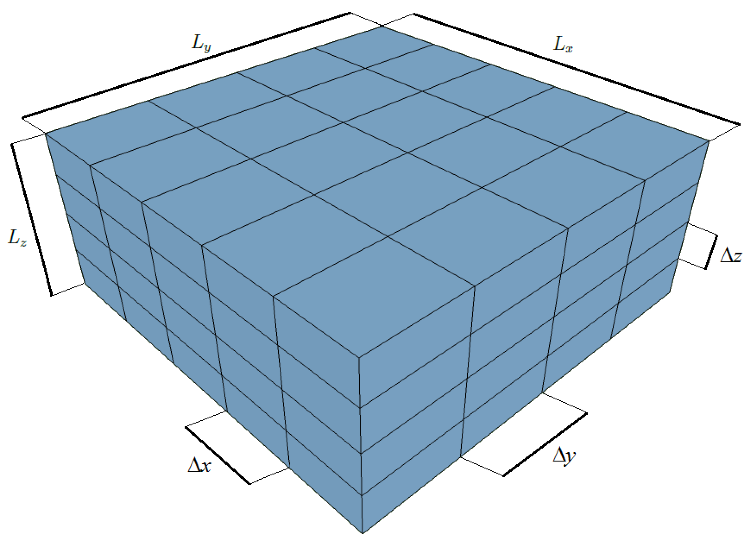
The domain of dimensions $L_x$, $L_y$, and $L_z$ is discretized using $n_x$, $n_y$, and $n_z$ finite volumes (whose dimensions, not necessarily constant, are $\Delta x$, $\Delta y$, and $\Delta z$) in the x-, y-, and z-directions, Figure 2, so that,

$$\sum _{i=1}^{n_x}\Delta x_i=L_x,\sum _{j=1}^{n_y}\Delta y_j=L_y,\sum _{k=1}^{n_z}\Delta z_k=L_z,$$

(23)

where the indices i, j and k indicate the blocks (cells or finite volumes) in the x-, y- and z-directions, respectively. In this system, we reference the boundaries (faces) of the blocks via the notation ($i\pm 1/2,j,k$), ($i,j\pm 1/2,k$), and ($i,j,k\pm 1/2$) [35].

In Figure 3, the faces of the finite volumes are indicated by $(i-1/2,j,k)=w$, $(i+1/2,j,k)=e$, $(i,j-1/2,k)=n$, $(i,j+1/2,k)=s$, $(i,j,k-1/2)=b$ and $(i,j,k+1/2)=a$. On the other hand, capital letters are used when referring to the nodes positioned at their respective centers: $(i-1,j,k)=W$, $(i-1,j,k)=E$, $(i,j-1,k)=N$, $(i,j+1,k)=S$, $(i,j,k-1)=A$, and $(i,j,k+1)=B$.

Once the computational mesh has been generated, space-time integration of Equations (13)–(15) is performed in each cell of the domain:

$$\begin{array}{ccc}\hfill {\int }_t^{t+\Delta t}{\int }_V{\displaystyle \frac{\partial }{\partial t}}\left[{\displaystyle \frac{\varphi \left(1-S_w\right)}{B_o}}\right]dVdt& \hfill =\hfill & {\int }_t^{t+\Delta t}{\int }_V\nabla ·\left[{\displaystyle \frac{k_{ro}}{{\mu }_o{B}_o}}\mathbf{k}\left(\nabla p_o-{\gamma }_o\nabla Z\right)\right]dVdt\hfill \\ \hfill & \hfill +\hfill & {\int }_t^{t+\Delta t}{\int }_V{q}_{s{c}_o}dVdt,\hfill \end{array}$$

(24)

$$\begin{array}{ccc}\hfill {\int }_t^{t+\Delta t}{\int }_V{\displaystyle \frac{\partial }{\partial t}}\left({\displaystyle \frac{\varphi S_w}{B_w}}\right)dVdt& \hfill =\hfill & {\int }_t^{t+\Delta t}{\int }_V\nabla ·\left[{\displaystyle \frac{k_{rw}}{{\mu }_w{B}_w}}\mathbf{k}\left(\nabla p_o-\nabla p_c-{\gamma }_w\nabla Z\right)\right]dVdt\hfill \\ \hfill & \hfill +\hfill & {\int }_t^{t+\Delta t}{\int }_V{q}_{s{c}_w}dVdt\hfill \end{array}$$

(25)

$$\begin{array}{ccc}\hfill {\int }_t^{t+\Delta t}{\int }_V{\displaystyle \frac{\partial }{\partial t}}\left[\left(\rho c_p\right)T\right]dVdt& \hfill =\hfill & {\int }_t^{t+\Delta t}{\int }_V\nabla ·\left[{\rho }_o{h}_o{\displaystyle \frac{k_{ro}}{{\mu }_o}}\mathbf{k}\left(\nabla p_o-{\gamma }_o\nabla Z\right)\right]dVdt\hfill \\ \hfill & \hfill +\hfill & {\int }_t^{t+\Delta t}{\int }_V\nabla ·\left[{\rho }_w{h}_w{\displaystyle \frac{k_{rw}}{{\mu }_w}}\mathbf{k}\left(\nabla p_o-\nabla p_c-{\gamma }_w\nabla Z\right)\right]dVdt\hfill \\ \hfill & \hfill +\hfill & {\int }_t^{t+\Delta t}{\int }_V\nabla ·(\mathbf{K}\nabla T)dVdt+{\int }_t^{t+\Delta t}{\int }_V{\displaystyle \frac{q_H}{V_b}}dVdt\hfill \\ \hfill & \hfill +\hfill & {\int }_t^{t+\Delta t}{\int }_V\left({\displaystyle \frac{{\rho }_o{h}_o{q}_{s{c}_o}}{V_b}}+{\displaystyle \frac{{\rho }_w{h}_w{q}_{s{c}_w}}{V_b}}\right)dVdt,\hfill \end{array}$$

(26)

where $\Delta t$ is the time increment and the subscript V indicates that the integration domain is the control volume.

Since a widely used method was chosen, the details concerning space-time integration of the governing equations will be omitted [30]. A fully time implicit formulation was opted for, and space-centered difference approximations were used.

In the discretized equations, a new variable, $\mathbb{T}$, representing the transmissibility evaluated on the faces of the finite volumes was introduced.

$${{\mathbb{T}}_{\alpha }}_e={\left({\displaystyle \frac{k_x{A}_x{k}_{r\alpha }}{{\mu }_{\alpha }{B}_{\alpha }\Delta x}}\right)}_e,{{\mathbb{T}}_{\alpha }}_w={\left({\displaystyle \frac{k_x{A}_x{k}_{r\alpha }}{{\mu }_{\alpha }{B}_{\alpha }\Delta x}}\right)}_w,$$

(27)

where the subscripts e and w refer to the values that must be evaluated on the $east$ and $west$ faces, $\Delta x_e$ and $\Delta x_w$ represent the distances between the centers of the cells neighboring the finite volume considered, and $A_x=\Delta x_P\Delta y_P$ is the area of the face of the finite volume. Analogous expressions are obtained for the other faces in the y- and z-directions.

Another point of fundamental importance is the approximation of transmissibilities at the interfaces of the control volumes. These terms can be highly nonlinear due to their dependence on the unknowns of the problem. This fact can generate problems with convergence, as reported in [36], and the stability of the numerical method. Knowing this context and remembering that the properties are defined at the centroid of the finite volume, appropriate approximations must be introduced to overcome these issues. First, $\mathbb{T}$ is calculated from the product between a geometric term, G, and two terms dependent on the dependent variables, $F_{(p,T)}{F}_S$. Then,

$$\mathbb{T}=G{F}_{(p,T)}{F}_S.$$

(28)

For example, the geometric terms appearing in the three balance equations are approximated on the east face e by

$$G_{xe}={\left({\displaystyle \frac{k_x{A}_x}{\Delta x}}\right)}_e={\displaystyle \frac{k_{xe}{A}_{xe}}{\Delta x_e}},$$

(29)

where the permeability, in turn, is determined via a harmonic mean

$$k_{xe}={\displaystyle \frac{k_{xP}{k}_{xE}\left(\Delta x_P+\Delta x_E\right)}{k_{xP}\Delta x_E+k_{xE}\Delta x_P}},$$

(30)

and the same type of approximation is used for the thermal conductivities that appear in the diffusion term of the energy equation.

The F terms can be computed in two different ways. For example, a centered difference scheme (uniform mesh) was used for those that are pressure- and temperature-dependent (weakly nonlinear).

$${\left(F_{(p,T)}\right)}_e={\displaystyle \frac{{\left(F_{(p,T)}\right)}_E+{\left(F_{(p,T)}\right)}_P}{2}},$$

(31)

while for the saturation-dependent terms, which are strongly nonlinear, it is done using a first-order upwind scheme. For example, for relative permeability

$$k_{r{\alpha }_e}=\{\begin{array}{cc}\hfill k_{r{\alpha }_P},& \mathrm{if}{v}_e\ge 0\\ \\ \hfill k_{r{\alpha }_E},& \mathrm{if}{v}_e<0\end{array}.$$

(32)

That is, it is the calculation of the relative permeabilities on the faces of the finite volumes. The capillary pressures on the faces are calculated analogously.

After carrying out all the steps recommended by the Finite Volume Method, the discretized form for the non-wetting phase (oil) was obtained [30]:

$$\begin{array}{cc}\hfill & \left(\sum _{d\in {\mathsf{\Omega }}_{face}}{\mathbb{T}}_{o_d}+M_{o_P}\right)p_{o_P}^{n+1}-{\left({\mathbb{T}}_o{p}_o\right)}_{Tot}^{n+1}-I_{o_{grav}}\hfill \\ =\hfill & \hfill M_{o_P}{p}_{o_P}^n-M_{o_T}\left(T^{n+1}-T^n\right)-\left(S_w^{n+1}-S_w^n\right)M_{o_S}+{\left(q_{s{c}_o}\right)}_P^{n+1}\hfill \end{array}$$

(33)

where ${\mathsf{\Omega }}_{face}$ refers to the set of faces of the finite volume, the term ${\left({\mathbb{T}}_o{p}_o\right)}_{Tot}^{n+1}$ is given by

$$\begin{array}{cc}\hfill {\left({\mathbb{T}}_o{p}_o\right)}_{Tot}^{n+1}& ={\left({\mathbb{T}}_{o_e}{p}_{o_E}\right)}^{n+1}+{\left({\mathbb{T}}_{o_w}{p}_{o_W}\right)}^{n+1}+{\left({\mathbb{T}}_{o_s}{p}_{o_S}\right)}^{n+1}\hfill \\ \hfill & +{\left({\mathbb{T}}_{o_n}{p}_{o_N}\right)}^{n+1}+{\left({\mathbb{T}}_{o_b}{p}_{o_B}\right)}^{n+1}+{\left({\mathbb{T}}_{o_a}{p}_{o_A}\right)}^{n+1}\hfill \end{array}$$

(34)

and with respect to gravitational effects,

$$I_{o_{grav}}={\mathbb{T}}_{o_a}^{n+1}{\gamma }_{o_a}^{n+1}\left(Z_P-Z_A\right)+{\mathbb{T}}_{o_b}^{n+1}{\gamma }_{o_b}^{n+1}\left(Z_B-Z_P\right).$$

(35)

The terms coming from the transient term are given by

$$M_{o_P}={\displaystyle \frac{V_b}{\Delta t}}{\left[\left(1-S_w^n\right)\left({\displaystyle \frac{c_{\varphi }{\varphi }^0}{B_o^n}}+{\displaystyle \frac{{\varphi }^{n+1}{c}_n}{B_o^0}}\right)\right]}_P,$$

(36)

$$M_{o_T}=-{\displaystyle \frac{V_b}{\Delta t}}{\left[\left(1-S_w^n\right)\left({\displaystyle \frac{c_{\varphi T}{\varphi }^0}{B_o^n}}+{\displaystyle \frac{{\varphi }^{n+1}{c}_{oT}}{B_o^0}}\right)\right]}_P,$$

(37)

$$M_{o_S}=-{\displaystyle \frac{V_b}{\Delta t}}{\left({\displaystyle \frac{\varphi }{B_o}}\right)}_P^{n+1},$$

(38)

where $V_b=\Delta x_p\Delta y_P\Delta z_P$.

Continuing, the discretized equation for the wetting phase (water) is presented [30]:

$$\begin{array}{cc}\hfill & {\left(\sum _{d\in {\mathsf{\Omega }}_{face}}{\mathbb{T}}_{w_d}{\displaystyle \frac{d{p}_{c_d}}{d{S}_{w_d}}}-M_{w_S}\right)}^{n+1}{S}_{w_P}^{n+1}-{\left(\sum _{\begin{array}{c}d\in {\mathsf{\Omega }}_{face}\\ D\in {\mathsf{\Omega }}_{vizinho}\end{array}}{S}_{w_D}{\mathbb{T}}_{w_d}{\displaystyle \frac{d{p}_{c_d}}{d{S}_{w_d}}}\right)}^{n+1}=M_{w_S}{S}_w^n\hfill \\ \hfill +& {\left(q_{s{c}_w}\right)}_P^{n+1}-{\left(\sum _{\begin{array}{c}d\in {\mathsf{\Omega }}_{face}\end{array}}{\mathbb{T}}_{w_d}\right)}^{n+1}{p}_{o_P}^{n+1}+{\left(\sum _{\begin{array}{c}d\in {\mathsf{\Omega }}_{face}\\ D\in {\mathsf{\Omega }}_{neighbor}\end{array}}{\mathbb{T}}_{w_d}{p}_{o_D}\right)}^{n+1}-\left(T^{n+1}-T^n\right)M_{w_T}\hfill \\ \hfill -& \left(p_o^{n+1}-p_o^n\right)M_{w_P}+I_{w_{grav}},\hfill \end{array}$$

(39)

where ${\sum }_{\begin{array}{c}d\in {\mathsf{\Omega }}_{face}\\ D\in {\mathsf{\Omega }}_{vizinho}\end{array}}$ refers to the summation on each face d and, at the same time, on each centroid of the neighboring cell D, for the same spatial direction. Furthermore, the gravity term is given by

$$I_{w_{grav}}={\mathbb{T}}_{w_b}^{n+1}{\gamma }_{w_b}^{n+1}\left(Z_B-Z_P\right)+{\mathbb{T}}_{w_a}^{n+1}{\gamma }_{w_a}^{n+1}\left(Z_A-Z_P\right),$$

(40)

and the other ones are

$$M_{w_P}={\displaystyle \frac{V_b}{\Delta t}}{\left[S_w^n\left({\displaystyle \frac{c_{\varphi }{\varphi }^0}{B_w^n}}+{\displaystyle \frac{{\varphi }^{n+1}{c}_w}{B_w^0}}\right)\right]}_P,$$

(41)

$$M_{w_T}=-{\displaystyle \frac{V_b}{\Delta t}}{\left[S_w^n\left({\displaystyle \frac{c_{\varphi T}{\varphi }^0}{B_w^n}}+{\displaystyle \frac{{\varphi }^{n+1}{c}_{wT}}{B_w^0}}\right)\right]}_P,$$

(42)

$$M_{w_S}={\displaystyle \frac{V_b}{\Delta t}}{\left({\displaystyle \frac{\varphi }{B_w}}\right)}_P^{n+1}.$$

(43)

Finally, the discretized form of the energy equation is presented [30]:

$$\begin{array}{cc}\hfill & {\left[\left(\rho c_p\right){\displaystyle \frac{V_b}{\Delta t}}+{\Gamma }^{\ast }\right]}^{n+1}{T}_P^{n+1}-{\Gamma }_e^{n+1}{T}_E^{n+1}-{\Gamma }_w^{n+1}{T}_W^{n+1}-{\Gamma }_s^{n+1}{T}_S^{n+1}-{\Gamma }_n^{n+1}{T}_N^{n+1}\hfill \\ \hfill -& {\Gamma }_b^{n+1}{T}_B^{n+1}-{\Gamma }_a^{n+1}{T}_A^{n+1}=I_{advec}^{n+1}-I_{grav}^{n+1}+I_{source}^{n+1}+{\displaystyle \frac{V_b}{\Delta t}}{\left(\rho c_p\right)}^n{T}_P^n\hfill \end{array}$$

(44)

where

$${\Gamma }^{\ast }=\sum _{d\in {\mathsf{\Omega }}_{face}}{\Gamma }_d,{\Gamma }_d={\displaystyle \frac{A_d{K}_d}{\Delta x_d}},$$

(45)

and the advective, gravitational and source terms are given, respectively, by

$$\begin{array}{ccc}\hfill I_{advec}^{n+1}& \hfill =\hfill & {\left[\left(\sum _{d\in {\mathsf{\Omega }}_{face}}{\rho }_{s{c}_w}{h}_{w_d}{\mathbb{T}}_{w_d}\right)p_{c_P}\right]}^{n+1}-{\left[\left(\sum _{d\in {\mathsf{\Omega }}_{face}}{\rho }_{s{c}_o}{h}_{o_d}{\mathbb{T}}_{o_d}+{\rho }_{s{c}_w}{h}_{w_d}{\mathbb{T}}_{w_d}\right)p_{o_P}\right]}^{n+1}\hfill \\ \hfill & \hfill +\hfill & {\left[\sum _{\begin{array}{c}d\in {\mathsf{\Omega }}_{face}\\ D\in {\mathsf{\Omega }}_{neighbor}\end{array}}\left({\rho }_{s{c}_o}{h}_{o_d}{\mathbb{T}}_{o_d}+{\rho }_{s{c}_w}{h}_{w_d}{\mathbb{T}}_{w_d}\right)p_{n_D}\right]}^{n+1}-{\left({\rho }_{s{c}_w}{h}_{w_d}{\mathbb{T}}_{w_d}{p}_{c_P}\right)}^{n+1},\hfill \end{array}$$

(46)

$$\begin{array}{ccc}\hfill I_{grav}^{n+1}& \hfill =\hfill & {\left({\gamma }_{n_b}{\mathbb{T}}_{n_b}{\rho }_{s{c}_n}+{\gamma }_{w_b}{\mathbb{T}}_{w_b}{\rho }_{s{c}_w}\right)}^{n+1}\left(Z_B-Z_P\right)\hfill \\ \hfill & \hfill +\hfill & {\left({\gamma }_{n_a}{\mathbb{T}}_{n_a}{\rho }_{s{c}_n}+{\gamma }_{w_a}{\mathbb{T}}_{w_a}{\rho }_{s{c}_a}\right)}^{n+1}\left(Z_A-Z_P\right),\hfill \end{array}$$

(47)

$$I_{source}^{n+1}=Q_H+{\left({\rho }_o{h}_o{Q}_{s{c}_o}\right)}^{n+1}+{\left({\rho }_w{h}_w{Q}_{s{c}_w}\right)}^{n+1}.$$

(48)

It is worth noting that the nonlinear system formed by these three equations is coupled since the oil pressure and water saturation depend on the average temperature value.

3.1. Operator Splitting and Linearization

Since linear algebra methods were chosen, the system of discretized equations must be linearized. To do so, the Picard Method was opted for [37],

$${\mathbb{T}}^{n+1}\approx {\mathbb{T}}^{n+1,v},$$

(49)

where ${\mathbb{T}}^{n+1,v}$ represents, for example, the transmissibility evaluated at time $n+1$, but at the previous iterative level v. On the other hand, the dependent variables are calculated at $n+1,v+1$, where $v+1$ is the subsequent iterative level. Therefore, an external iterative process linked to the Picard Method and an internal one for the numerical resolution of the system of discretized equations are present.

However, in the present work, an Operator Splitting Method was employed [38,39] to enable the unknowns of the system to be determined by solving the equations sequentially. Thus, it was possible to arbitrate the most appropriate algebraic methods for each of them [36].

The following resolution order was established [30]:

• firstly, the subsystem that will provide the pressure of the non-wetting phase is solved (Equation (33));
• next, the saturation of the wetting phase is obtained (Equation (39));
• finally, the average temperature of the reservoir is determined (Equation (44)).

The application of operator splitting with the use of two fully implicit numerical formulations aims, in the case of the pressure formulation, to benefit from the efficient design inherent in the IMPES method, while the use of implicit formulations for saturation and temperature avoids severe time-step restrictions such as those that occur in the IMPES method due to the explicit formulation for saturation. Furthermore, the splitting as utilized allows the Conjugate Gradient method to be applied for the solution of pressure and temperature, with the Biconjugate Conjugate Gradient method being necessary only for the determination of water phase saturation. This reduces the computational cost compared to a solution using a Fully Implicit Method methodology.

3.2. Resolution of Linear Algebraic Systems

Due to the strategy employed in solving the governing equations, the pressure and average temperature are determined via the Preconditioned Conjugate Gradient Method [6], while the saturation is obtained using the Preconditioned Stabilized Biconjugate Gradient Method [40].

The choice of preconditioned methods was based on the possibility of accelerating the convergence process of iterative methods. To this end, preconditioners constructed from the incomplete LU Factorization process were used [40].

4. Numerical Results

This section aims to present and discuss the results obtained, which are the calculated values for variables dependent on oil pressure, water saturation, and average reservoir temperature. Prior to the discussion, validation of the numerical method was performed.

For the scenario under consideration, a well-reservoir coupling technique is not employed for well modeling, nor is a simplified representation via source/sink terms utilized. Given the adoption of a slab geometry, the flow is governed by the direct influence of boundary conditions.

4.1. Numerical Verification

A non-isothermal one-dimensional flow problem was selected to verify the accuracy of the results for two-phase flow. The selection of this example was driven by its analytical solution, coupled with the ability to simplify the simulator’s original operational conditions to obtain results suitable for a comparative analysis of a non-isothermal two-phase flow scenario.

To this end, the analytical solution of a simplified dimensionless problem, the soil remediation process, was utilized. This process consists of injecting liquid water into a porous medium to remove oil in the soil. The fluids are immiscible, and the effect of capillarity on the flow was not considered.

The effects of capillary pressure are disregarded, the fluids have approximately the same thermal capacity, and energy transfer by diffusion was neglected. Therefore, after simplifications [41]

$${\displaystyle \frac{\partial T}{\partial t}}+{\displaystyle \frac{\partial T}{\partial x}}=0,-\infty <x<\infty ,$$

(50)

subject to a Riemann-type initial condition

$$T(x,0)=\{\begin{array}{cc}\hfill 1,& x<0\\ \hfill 0,& x>0\end{array}.$$

(51)

Therefore, the solution in terms of temperature is a discontinuity that advances through the porous region. Notably, viscosity influences the flow pattern as a temperature-dependent property [41]

$${\mu }_n\left(T\right)=\left(1-\delta \right)exp\left(T-1\right)+\delta ,$$

(52)

where ${\mathsf{\mu }}_n$ is the viscosity of the non-wetting phase, $\delta$ is equal to 1/523, and the viscosity of the wetting phase is assumed to be 1 [41].

To determine the saturation (S), two regions separated by the temperature discontinuity interface must be considered: one on the left (higher temperature) and the other on the right (lower temperature). Therefore [41],

$${\displaystyle \frac{\partial S_1}{\partial t}}+{\displaystyle \frac{\partial f_1}{\partial x}}=0,-\infty <x<t,$$

(53)

for the first region, subscript 1, and

$${\displaystyle \frac{\partial S_2}{\partial t}}+{\displaystyle \frac{\partial f_2}{\partial x}}=0,t<x<\infty ,$$

(54)

for the second region, subscript 2, and they must be solved considering the following initial condition

$$S(x,0)=\{\begin{array}{cc}\hfill 1,& x<0\\ \hfill 0,& x>0\end{array}.$$

(55)

In Equations (53) and (54), $f_1$ and $f_2$ represent the respective flux functions that, for the adopted assumptions [41], are given by

$$f_1={\displaystyle \frac{S^3}{S^3+\delta {\left(1-S\right)}^3}},x<t$$

(56)

and

$$f_2={\displaystyle \frac{S^3}{S^3+\delta exp\left(1\right){\left(1-S\right)}^3}},x>t.$$

(57)

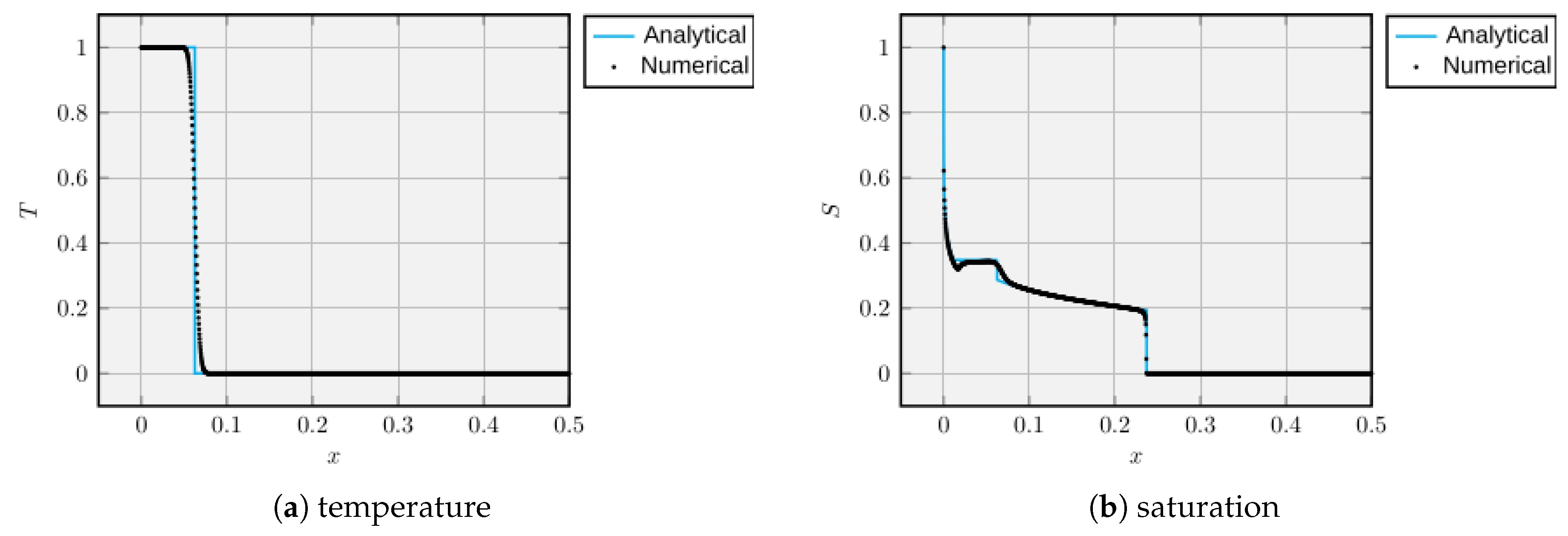
The saturation and temperature profiles can be observed in Figure 4a and Figure 4b, respectively, obtained with a grid containing 1000 cells and a time increment equal to 0.0025. The figures also represent the analytical solutions determined by Moyles [41] for t = 0.0625.

For temperature, a comparison between numerical and analytical results shows that the simulator correctly captured the jump that occurs at $x=t$. Nevertheless, due to numerical diffusion, a slight, noticeable effect is present. However, spurious oscillations are absent, which, according to Pletcher et al. [42], would be undesirable when solving a problem containing discontinuities in its solution, which must be reproduced numerically as accurately as possible. The temperature values are independent of those of saturation, but modify them since the viscosity varies with the temperature.

Regarding the saturation profile, it is possible to see that, in general, the same behavior was observed for both the numerical and analytical values. In the first rarefaction, they are superimposed. However, at the end of it, a deviation is noticed, and the numerical results are below the predicted value, similar to what occurs numerically in Moyles [41]. After the first rarefaction, the saturation value remains constant until the appearance of the first shock. In the case of the analytical solution, the discontinuity is visible, but it is smoothed out due to numerical diffusion in the results. It is worth noting that the appearance of the shock is due to the change in the fluid viscosity, showing the existence of coupling of the equations. After the formation of the first shock, a second rarefaction begins, followed by the appearance of the last shock.

Despite the influence of numerical diffusion, the numerical results are considered to have adequately reproduced those predicted by theory.

The case considered in this paper is more realistic and complex than that of the example for which an analytical solution is known. Consequently, we were compelled to resort to a numerical solution.

4.2. Sensitivity Analysis

Continuing, the study of the thermal oil recovery process is addressed. The problem of injecting heated water into a reservoir with a slab-type geometry was considered. This procedure aims to sweep the oil still in the reservoir towards the production region, besides reducing its viscosity and favoring the flow of fluids in this region. It is a fundamental case for sensitivity analysis and has significant relevance in the hydrocarbon recovery process, highlighting the contribution of the effects of heating in the recovery of, for example, heavy oil.

This study allows for understanding what happens in a complex process of injecting heated water into a heavy oil reservoir. Therefore, to better understand it, the focus is on understanding the influence of the effect of the variation of the water injection temperature ($T_{inj}$), oil viscosity, and the water injection rate (${\partial p/\partial x|}_{x=0}$).

The listed aspects were used as an integral part of the sensitivity analysis process. The standard model for the simulations includes a reservoir containing water and oil, with a three-dimensional geometry in the form of a parallelepiped, whose dimensions are defined by the values of its length, width, and height, respectively $L_x$, $L_y$, and $L_z$ provided in

Table 1. Parameters for the reservoir.

Parameter	Value	Unit
$k_x=k_y$	2.9 10−15	$\mathsf{\mu }$m2
$k_z$	7.35 10−16	$\mathsf{\mu }$m2
$L_x$	609.6	m
$L_y$	304.0	m
$L_z$	30.4	m
${\varphi }_{ini}={\varphi }^0$	0.2	-

. In this table, $k_x$, $k_y$, and $k_z$ represent the permeability values in the directions of the x, y, and z axes, respectively, and ${\varphi }_{ini}$ is the initial value of the reservoir porosity.

Table 2. Parameters for numerical simulations.

Parameter	Value	Unit
$F_{{\Delta }_t}$	1.1	-
$n_x$	250	-
$n_y$	50	-
$n_z$	5	-
${p|}_{x=L_x}$	4.0 104	kPa
$p_{ini}=p^0$	4.0 104	kPa
$S_w^0$	0.2	-
$S_w{|}_{x=0}$	0.85	-
$t_{max}$	7000	day
$T_{inj}$	400	K
$T_{r_{ini}}$	340	K
$\Delta t_i$	1.0 10−2	day
$\Delta t_f$	10	day
${\partial p/\partial x|}_{x=0}$	$-10$	kPa/m
$\partial S_w{/\partial x|}_{x=L_x}$	0.0	-
${\partial T/\partial x|}_{x=L_x}$	0.0	K/m

,

Table 3. Parameters for fluids.

Parameter	Value	Unit
$a_n$	5.0 10−5	Pa·s
$b_n$	444.4	K
$B_o^0={\rho }_{sco}/{{\rho }_o}^0$	1.13	-
$B_w^0={\rho }_{scw}/{{\rho }_w}^0$	1.022	-
$c_o$	7.25 10−7	kPa−1
$c_{oT}$	1.2 10−3	K−1
$c_{p_o}$	1700	J·K−1·Kg
$c_{p_w}$	4128.18	J·K−1·Kg
$c_w$	2.61 10−6	kPa−1
$c_{wT}$	2.07 10−5	K−1
$T_{ref}$	277.78	K
${\kappa }_o$	0.1225	W·m−1·K−1
${\kappa }_w$	0.6	W·m−1·K−1
${\mathsf{\mu }}_w$	0.00069	Pa·s
${\rho }_o^0$	959	kg/m3
${\rho }_w^0$	1000	kg/m3

and

Table 4. Parameters for the porous matrix.

Parameter	Value	Unit
$c_{p_r}$	1200	J·K−1·Kg
$c_{rT}$	1.8 10−5	K−1
$c_{\varphi }$	5.8 10−7	kPa−1
$d_p$	1.0 10−4	m
$epc$	2	-
$ew=eow$	4	-
$p_{c_{max}}$	39.98	kPa
$S_{iw}$	0.15	-
$S_{ro}$	0.15	-
${\kappa }_r$	4.5	W·m−1·K−1
${\rho }_r$	2500	kg/m3
$|\nabla G|$	30	K/km

also contain several parameters used in the simulations, the default case, besides the properties of the fluids and the rock. Unless explicitly mentioned, these were the values used in all simulations. In Table 2, $\Delta t_i$ is the initial time step, $\Delta t_f$ is the final time step, and $F_{{\Delta }_t}$ is the rate of increase of the time increment ($\Delta t^{n+1}=F_{{\Delta }_t}\Delta t^n$). Furthermore, $p_{ini}$ indicates the initial pressure at the top of the reservoir, $S_w^0$ the initial water saturation, $t_{max}$ the maximum production time, and $T_{r_{ini}}$ the initial temperature of the rock. The properties and parameters used in the simulations were based on those available in the work of the author dos Santos Heringer et al. [39]. It is noteworthy that the computational mesh was selected following a mesh refinement study [30]. For numerical methods that are consistent and stable, it is well-established that a reduction in spatial increments leads to a decrease in truncation error and an increase in accuracy [35].

4.2.1. Variation of Injected Fluid Temperature

As previously mentioned, an increase in heavy oil temperature reduces its viscosity and alters the saturation curve. Therefore, simulations with varying water injection temperatures were performed to examine the behavior of pressure, saturation, temperature, and viscosity within the reservoir. Figure 5 depicts pressure values along the x axis, obtained by injecting water at distinct temperatures for a final production time ($t_{max}$) of 7000 days.

Figure 5 shows that higher injection temperatures result in higher reservoir pressures. This occurs due to the reduction in oil viscosity, facilitating the introduction of a greater quantity of water, which increases reservoir pressure. Notably, in the inlet region on the left, the pressure on the injection face exhibits very similar values due to the equivalent relative permeability at the same saturation value for each temperature. However, a slight difference remains, with marginally higher pressures at lower temperatures. This is attributed to increased resistance to water entry, leading to a consequent rise in inlet pressure to maintain the pressure gradient.

Regarding temperature, as expected, higher water injection temperatures lead to increased reservoir temperatures across all regions, though decreasing with distance from the injection region. This results in an approximate 12 K increase between minimum and maximum values for regions 100 m from the injection boundary.

Analysis of the results indicates that increasing injection fluid temperature leads to greater oil recovery and higher water presence near the injection boundary. This is a direct consequence of the temperature-induced decrease in oil viscosity due to energy transfer from the wetting phase. Ultimately, this represents the practical outcome of thermal recovery via heated fluid injection. The importance of thermal methods in heavy oil recovery is evident here. The heating-induced reduction in oil viscosity increases sweep efficiency.

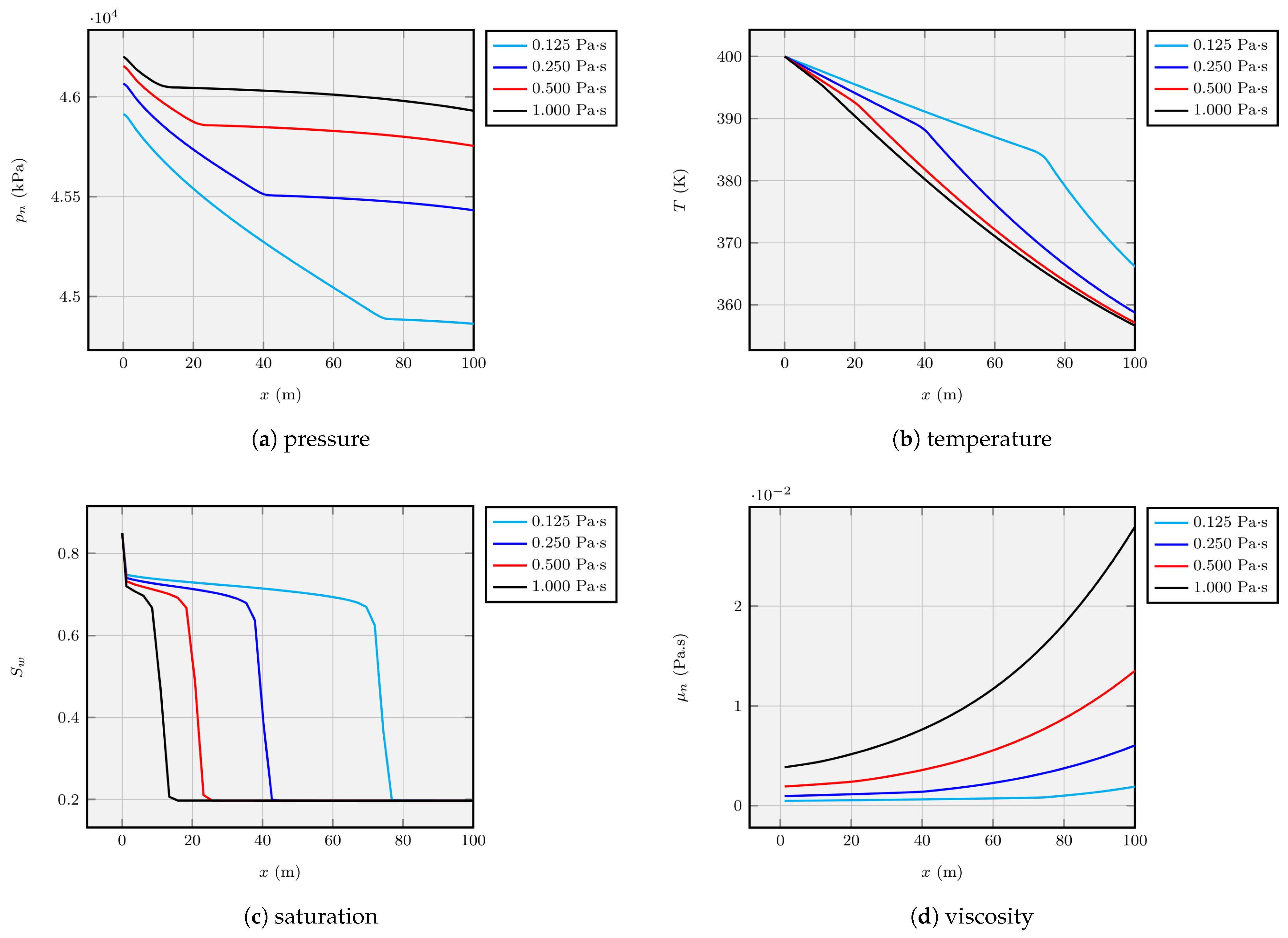
4.2.2. Oil Viscosity Variation

The variation in oil viscosity as a function of injected fluid temperature changes (Figure 6) confirms previous assertions. The heated fluid decreases oil viscosity due to increased temperature. Since the injected water is confined to a region less than 20 m from the injection boundary, the oil viscosity decrease is also greater in this region, progressively increasing with distance. The diminished viscosity increases oil mobility within the reservoir. Water viscosity was assumed constant despite temperature variations, thus its changes were disregarded relative to those of the oil. The parameter $a_n$ of Equation (4) directly affects oil viscosity. Consequently, its influence on pressure, saturation, temperature, and oil viscosity was studied. Unlike the previous case, where viscosity changes were confined to the heated region, the effect of viscosity variation throughout the entire reservoir was analyzed. Four different values of $a_n$ were chosen, and the same trends were observed compared to the previous results.

Analysis of the pressure curves reveals that increased viscosity causes a considerable pressure rise in the injection region and the rest of the reservoir. This is attributed to reduced fluid mobility with increased viscosity, necessitating higher injection pressure to maintain the same pressure gradient. Consequently, lower oil viscosity results in lower flow resistance and pressure values.

Regarding temperature results, Figure 6 shows that higher viscosity leads to lower medium temperatures. This can be explained by reduced fluid mobility, resulting in decreased velocity and Péclet number. Thus, heat transfer by advection is reduced in flows of more viscous fluids compared to those of lower viscosity.

Additionally, the results show a higher amount of residual oil with increased oil viscosity, explained by the higher flow resistance experienced by more viscous fluids. Analysis of saturation variation shows that, as expected, the advanced front of the injected fluid progresses less for more viscous fluids, advancing more slowly. Conversely, for less viscous oils, distant regions are reached by the injected fluid within the same time period.

The results also confirm the effects of the parameter $a_n$ on oil viscosity. Higher values of $a_n$ result in higher fluid viscosity throughout the reservoir. However, due to heating of the injected fluid near the injection region, viscosity assumes lower values and increases with distance from the reservoir’s left border.

It is relevant to highlight that viscosity varies differently as a function of temperature for each specific oil. Therefore, unlike water injection temperature, the viscosity variation pattern cannot be changed unless the oil’s physical properties are modified by injecting specific products.

4.2.3. Injection Rate Variation

The water injection rate is another fundamental parameter for this study, as it defines the volume of water injected into the reservoir. The respective curves obtained by changing the injection rate are shown in Figure 7, for the variation of pressure, temperature, saturation, and viscosity.

Reduced injection rates result in decreased water injection, leading to lower water saturation and consequently, increased capillary pressure. Since oil pressure is the sum of water pressure and capillary pressure, oil pressure increases. Within the tested range, the capillary pressure difference is sufficient to elevate oil pressure in the region downstream of the displacement front when lower injection rates are applied. Upstream of the displacement front, reduced injection rates result in a smaller increase in oil pressure, indicating that the imposed rate change, rather than the capillary pressure variation, is the dominant factor in this region. However, the pressure profile tends toward stabilization with the prescribed pressure condition at the $x=L_x$ boundary, coupled with the imposed injection rate, as observed for higher injection rates.

From Figure 7, regarding temperature curves, it can be concluded that the variation in heated fluid injection rate did not cause significant changes in average reservoir temperature values. Consequently, substantial changes in oil viscosity values are not expected.

Examination of the saturation curves demonstrates the positive impact of an initial increase in the injection rate, leading to improved sweep efficiency. However, with further increases in the injection rate, the water fronts advance at increasingly similar velocities, and the saturation curves become progressively closer. Therefore, the residual oil volume within the swept region tends to be the same for higher injection rates.

For the evaluated cases, based on the observed temperature variation inside the reservoir, the viscosity curves are verified to be practically identical regardless of injection rate values.

5. Conclusions

A numerical simulator was developed to solve the problem of non-isothermal three-dimensional two-phase flow in an oil reservoir, and the subsystems for oil pressure, water saturation, and average temperature were solved sequentially. The coefficients of the equations appearing in these subsystems are linearized using the Picard method, and pressure and water saturation were calculated implicitly. When calculating average temperature, the hypothesis of local thermal equilibrium was not considered, and an implicit formulation in time was also used. The effects of tortuosity and hydrodynamic dispersion are accounted for.

The numerical code was validated based on a problem with a known analytical solution from the literature. Its resolution verified numerical convergence and showed that the numerical results reproduced those provided by theory. However, a small smoothing due to numerical diffusion caused by the first-order upwind scheme was observed.

Unquestionably, variation of the injection temperature proved to be the most efficient technique for oil recovery in the tested cases in the sensitivity analysis, considering the water saturation value at the end of the rarefaction curve. Higher temperatures resulted in a reduction in viscosity and the amount of oil found in the region swept by the heated water.

In the other cases, comparable practical gains in swept efficiency were not obtained despite the reduction in oil viscosity. In the first test case, variation of injected fluid temperature, the water saturation immediately before the discontinuity, which defines the position of the advancing front, increased from approximately 0.55 to 0.65 for the lowest and highest water injection temperatures, an increase of about 18%.

Overall, the sequential method and the methodologies for discretization, linearization, and solution of algebraic systems proved effective when applied to the problem of non-isothermal two-phase flow.

The findings indicate that increased reservoir temperature, including in regions located near producing wells (currently under investigation), serves as a viable strategy to enhance oil recovery, such as heavy oil. The primary mechanism is the temperature-mediated reduction of oil viscosity, which results in a decrease in flow resistance and an increase in fluid mobility. Hence, this underscores the necessity of research into non-isothermal flow and thermal enhanced oil recovery strategies.

To address problems closer to those encountered in real situations, we are currently working on including well-reservoir coupling, the possibility of dissolved gas, and the simulation of isothermal three-phase flow. In the future, we also plan to consider the case of non-isothermal three-phase flow.