Experimental Research of the Possibility of Applying the Hartmann–Sprenger Effect to Regulate the Pressure of Natural Gas in Non-Stationary Conditions

Abstract

This research focuses on the development of a quasi-isothermal pressure regulator based on the principle of flow mixing after energy separation. Currently, no established methods exist for designing pressure reduction devices that utilize energy separation effects, and this study aims to fill this gap. The paper presents experimental results on the performance of a pressure reduction device operating based on the Hartmann–Sprenger effect. This study investigated the hypothesis that by selecting the size of resonators, relative distances, and their mutual location, it would be possible to realize pressure regulation, simultaneously providing both the maintenance of a significant effect and the full provision of the functions of pressure regulators operating in non-stationary conditions. The experiments involved three resonators (45.5 mm, 70.5 mm, and 97.5 mm) in regurgitant mode. The findings revealed that the smallest resonator demonstrated the highest rate of temperature increase, with an average value of 2.36 K/s. The medium resonator exhibited the highest reliability under non-stationary conditions, while the largest resonator provided the highest temperature, with a maximum excess of 102 K over the temperature in front of the nozzle. The primary goal of this study was to develop technology suitable for installation at a pressure reduction station, considering mass and dimensional constraints.

1. Introduction

As global decarbonization efforts advance and renewable energy solutions continue to spark debate [1], natural gas is emerging as a crucial component of the energy mix. However, the production of natural gas is increasingly challenged by the depletion of easily accessible reserves, shifting the focus toward hard-to-recover and unconventional hydrocarbons. These hard-to-recover gas accumulations, which exist under varying thermobaric conditions, are difficult and inefficient to extract using current technologies. This geological issue significantly impacts the profitability of global liquefied natural gas (LNG) projects, particularly in Russia, where tax incentives for hard-to-recover gas remain underdeveloped compared to those for oil reserves.

The current approach to evaluating hard-to-recover reserves primarily focuses on permeability (e.g., shale or tight gas) while overlooking critical factors such as reservoir pressure and depth. Extracting gas from deep or low-pressure reservoirs requires specialized and costly equipment. Consequently, a comprehensive strategy is needed to address the geological, technological, and economic challenges associated with hard-to-recover gas. Such a strategy would involve optimizing gas transportation infrastructure and refining LNG production processes to ensure the continued viability of natural gas in both domestic and global markets.

Russia’s growing natural gas portfolio, supported by both pipeline and LNG transport developments, highlights the importance of advancing technologies to minimize capital and operational expenditures. As reserves deplete and production costs rise, efficient solutions for gas transportation and distribution, such as the Hartmann–Sprenger effect for pressure reduction, will play a key role in maintaining profitability.

Long-distance gas transportation requires high pressure to reduce hydraulic losses and increase the mass of the transported gas. Such an approach necessitates pressure reduction before supplying gas to the final consumer. Gas pipelines are categorized according to the pressure of the transported gas, with pressure gradually decreasing as it approaches the final consumer. For example, in the Russia, the following classification is applied [2]: high 1—from 0.6 to 1.2 MPa; high 2—from 0.3 to 0.6 MPa; medium—from 0.005 to 0.3 MPa; and low—up to 0.005 MPa, inclusive. Thus, there can be up to four stages of pressure reduction. There are more than 350,000 natural gas pressure reduction points in the Russia.

Gas pressure is reduced by converting pressure energy to overcome local resistance in the form of a valve-type throttle valve. According to the Joule–Thomson effect, the pressure drop causes a temperature reduction, which can lead to the precipitation of gas hydrates. To prevent such negative consequences, the transported gas is heated to maintain the temperature at a level no lower than −10 °C, or 0 °C on heaving soils. Usually, a portion of the transported gas (about 0.3% of the total amount) is burned for this purpose.

Such an approach seems ineffective, as energy is lost during the reduction process, and then additional energy must be supplied to restore the temperature.

Obviously, the most effective solution to the above problem is to utilize the energy of the gas flow itself and convert it into heat.

The most promising yet least studied is the Hartmann–Sprenger resonance effect [3,4].

2. Overview of the Hartmann–Sprenger Effect

The supersonic gas flow around a closed cavity induces self-oscillating gas pressure fluctuations inside it. As a result of cumulative heat supply, the temperature at the dead end of the resonator rises [5] due to the interactions of shock waves propagating inside the resonator [6,7] and the friction of the gas against the walls [8]. This leads to high temperatures being achieved with a low cooling capacity [9], making it possible to use such a device for gas pressure reduction.

Due to its temperature performance (temperatures up to 1600 K [10] and heating rates up to 160 K/ms [11]), the effect has found wide application in detonation systems for warheads [12] and rocket engine ignition systems [13,14,15]. Additionally, the effect is used in electricity generators based on thermoelectric elements [16], thermal desorption [17], magnetohydrodynamic energy conversion [18], and acoustic agglomeration [19].

Typically, scientists study this effect as a negative one and attempt to exclude it, for example, in aircraft engineering, as it causes the unacceptable heating of supersonic aircraft structural elements. Recently, with the increasing operating pressure of new gas pipelines, instances of heating in risers of block valve stations have become more frequent [20].

There are three operating modes of the nozzle–resonator pair [21,22]:

• Instability of the flow: This mode occurs at subsonic speeds. Due to the formation of vortices at the nozzle outlet, the flow is unable to generate strong shock waves in the resonator, resulting in no significant heating of the gas [23].
• Regurgitation of the flow: In this mode, the resonator periodically ingests and emits portions of gas. The flow structure can form diamond-shaped or barrel-shaped cells, depending on the pressure difference across the nozzle. This mode is most effective with long resonators, as more space is required for the superposition of compression waves and the formation of strong shock waves. However, this mode does not allow for the achievement of significant temperatures or heating rates.
• Screech of the flow: This mode requires relatively high flow pressure before the nozzle. It is characterized by the formation of a Mach disk (normal shock wave) at the resonator inlet, which oscillates at a higher frequency than in other modes. However, the shock waves become weaker. In this mode, maximum temperatures can be achieved, as the mass exchange between the hot gas trapped in the tube and the cold flow around the resonator is reduced. This mode is optimal when working with relatively short resonators [21,22].

The structure of the under-expanded jet [24] and the location of the “instability” zones depend on the pressure drop across the nozzle and the degree of deviation from the design ($n=p_n/p_a$, where $p_n$ and $p_a$ are the pressures in the nozzle outlet and the surrounding space, respectively). Depending on this, the optimum position of the resonator changes, and a decision must be made as to whether to place it inside or near [25] the first [26] or the second instability zone [23]. The resonator must be placed with the open end coaxially aligned with the nozzle to ensure the occurrence of the effect.

The optimum position can change depending on the flow parameters. If the pressure before the nozzle increases, the jet cells stretch, and the resonator must be placed farther from the nozzle; conversely, if the pressure decreases, the resonator should be placed closer [26]. Additionally, the transition from regurgitant mode to screech mode requires higher pressure in front of the nozzle, as the distance between the nozzle and the resonator increases [21]. The maximum temperature and heating rate are directly affected by the position of the resonator relative to the nozzle [27].

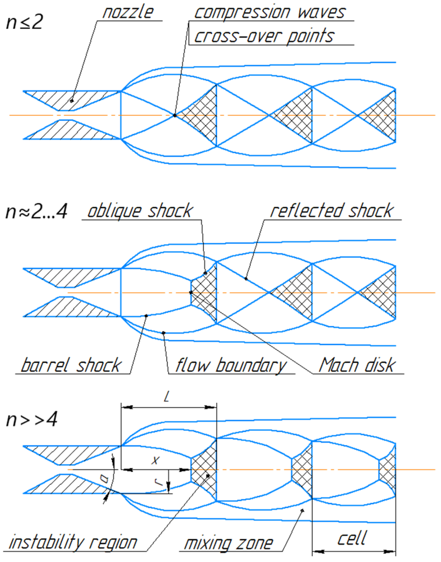
Depending on the degree of deviation $n$, the flow structure changes its shape. For $n\le 2$, the compression shocks have the diamond-shaped form (Figure 1); for $n=2\dots 4$, the first compression wave cell takes the barrel-shaped form with a Mach disk; with a further increasement ($n>4$), a high amount of Mach can form one after another in the cells. However, further growth of the value of $n$ will lead to the further growth of the thickness and diameter of the first Mach disk and, accordingly, will make it impossible for the following disks to appear [28]:

There are several ways to determine the flow structure. The first method is schlieren photography, but it is labor-intensive. The second method is analytical calculation based on a flow structure prediction model [28]. In the case of a flow structure with barrel-shaped compression shocks, the position of the direct compression shock (Mach disk) must be calculated to determine the boundaries of the “instability” zone. For diamond-shaped shock cells, the position of the inclined shock wave intersection point should be calculated. Depending on the pressure drop across the nozzle and the total pressure, an empirical formula can be used to determine the position of the Mach disk [29] (most of these formulas apply only to converging nozzles). According to E. Brocher and C. Maresca [25], the optimal ratio of the distance from the converging nozzle to the resonator and the diameter of the resonator in the subsonic regime is approximately 1. For the supersonic regime (Mach number equals 2), it is about 2 for a diatomic gas and about 3 for a monatomic gas. In the case of diffuser nozzles and barrel-shaped compression shocks, the position $x$ of the Mach disk (Figure 1) is calculated as [30,31]:

$$x=0.8L,$$

(1)

$$L=1.558·x\prime ,$$

(2)

$${\displaystyle \frac{x\prime }{r}}~\sqrt{n\left(1+k{M}^2\cos a\right)-1},$$

(3)

where $L$ is the length of the first cell; $M$ is the Mach number in the outlet section of the nozzle; $r$ is the radius of the outlet section of the nozzle; $k$ is the adiabatic exponent; and $a$ is nozzle half-opening angle. The intersection point of the inclined shock waves for a flow structure with diamond-shaped shocks will be located approximately in the middle of the cell. Nozzles with more complex geometries require numerical calculation methods.

Currently, the effects of energy separation are not widely used for the utilization of the pressure energy of natural gas. This is due to several major issues:

• The physics of the processes are not sufficiently studied.
• There are a lack of clear methods for designing devices based on these effects.
• Real-world production requires devices that can function under non-stationary conditions.

There are many studies that provide experimental data and general recommendations, but there are no structured algorithms or techniques for practical application.

In particular, the design of the pressure reduction device based on the Hartmann–Sprenger effect must address the following problems:

• How certain configurations of the device affect the attained temperature.
• How to determine the number of nozzle–resonator pairs and their parameters based on flow rate and pressure drop.
• How to ensure the stable performance of nozzle–resonator pairs under non-stationary conditions.
• How nozzle–resonator pairs interact when placed near each other.
• What the noise, vibration levels, and lifespan of such devices will be.

3. Core of the Proposal

The main idea behind using the Hartmann–Sprenger effect is that, during gas pressure reduction, pressure energy is not wasted but rather transformed into heat, which helps to reduce the drop in gas temperature after reduction.

The relationships used to determine the ratio of heat capacity to cooling capacity for the Hartmann–Sprenger effect are similar to those used to describe energy separation in Ranque–Hilsch vortex tubes [32,33,34,35].

It may seem that there would be little difference in gas cooling using this effect compared to conventional throttling.

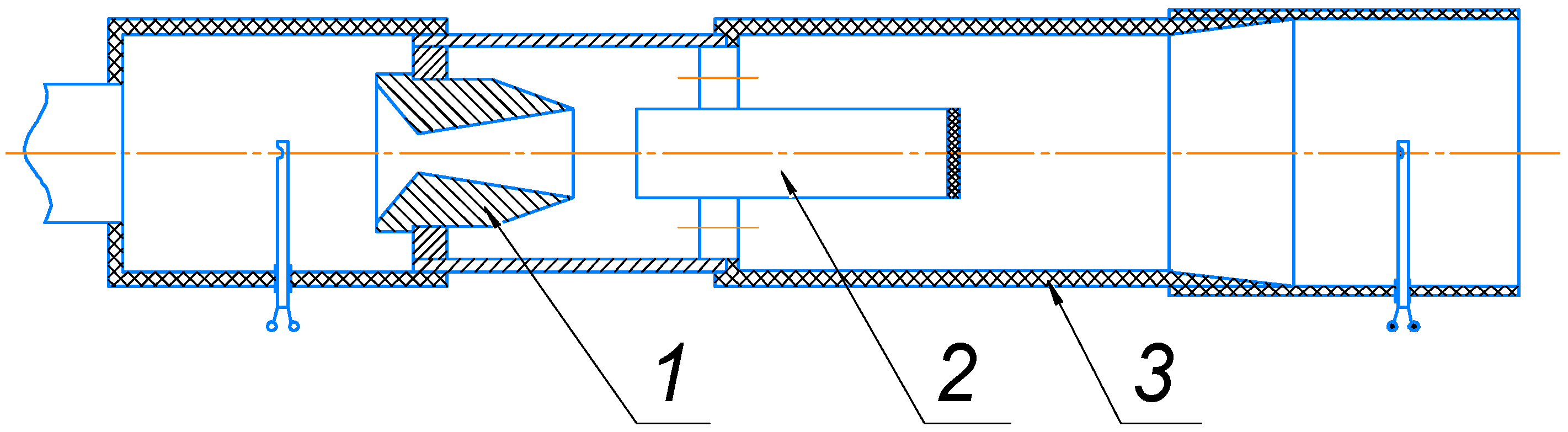
The simplest configuration involves mixing portions of gas, leaving the hot cavity with the flow around the resonator, while simultaneously providing heat exchange between the hot end of the resonator and the external flow (Figure 2).

Publications indicate that, after passing through the device, the temperature of dry air increases by up to 15 °C [36] for such a configuration. Theoretically, based on theoretical calculations, when the pressure decreases by 50 times, the temperature of natural gas after mixing hot and cold flows at the exit can reach a maximum value of 1.4 times the flow stagnation temperature. However, the limited amount of experimental data on flow mixing does not allow for any clear conclusions to be drawn.

This scheme (Figure 2), which employs only one nozzle–resonator pair, cannot be used in a gas distribution system, as the large length of the device would require significant modifications to the facility (the device length would be about 4 m at a flow rate of 50,000 m³/h) and it cannot operate under non-stationary conditions. During peak gas consumption hours, the gas flow through the device can change by 2 times [37]. Additionally, pressure fluctuations both before and after the pressure regulator must be considered.

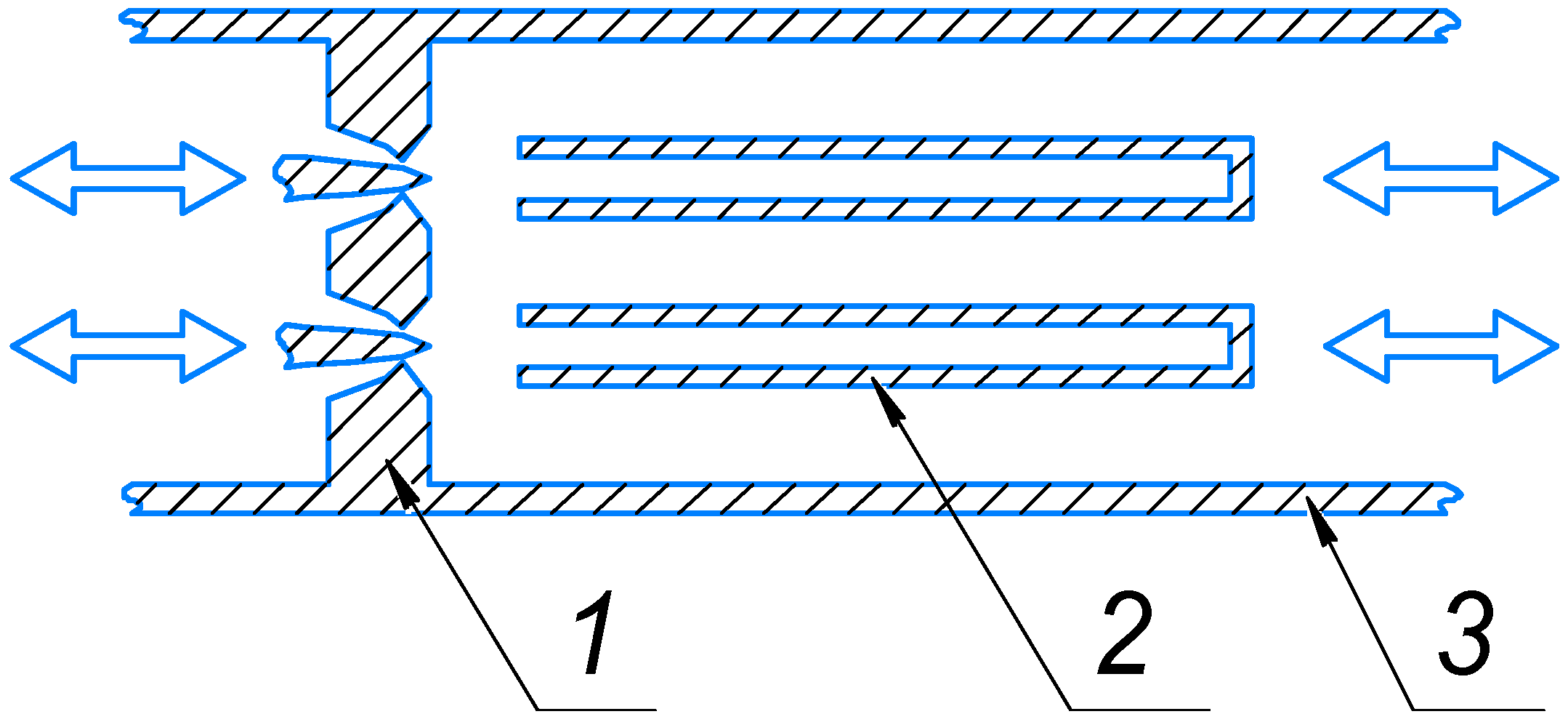
For pressure reduction purposes, it is proposed to use devices with multiple nozzle–resonator pairs, featuring an annular adjustable nozzle and resonators with a variable distance from the nozzle. Dividing the flow into several nozzle–resonator pairs will significantly reduce the dimensions of the device, making it possible to use it at reduction points while also ensuring more uniform heat exchange. The adjustable annular nozzles allow for the regulation of the gas flow by altering the flow section of the nozzle through the movement of the central body. The position of the resonator adjusts based on the flow structure to ensure the optimal operation of the device (Figure 3).

4. Experimental Methodology

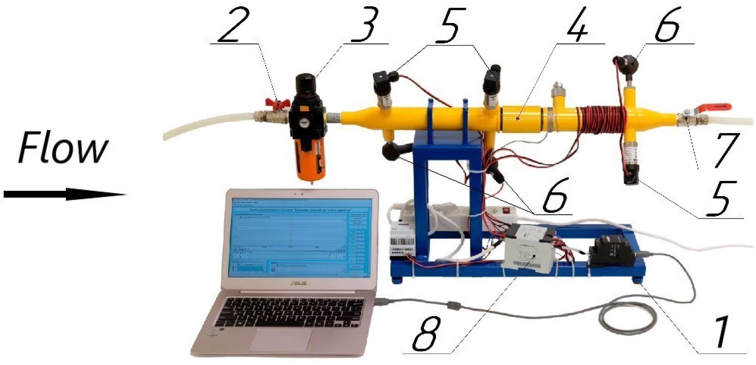
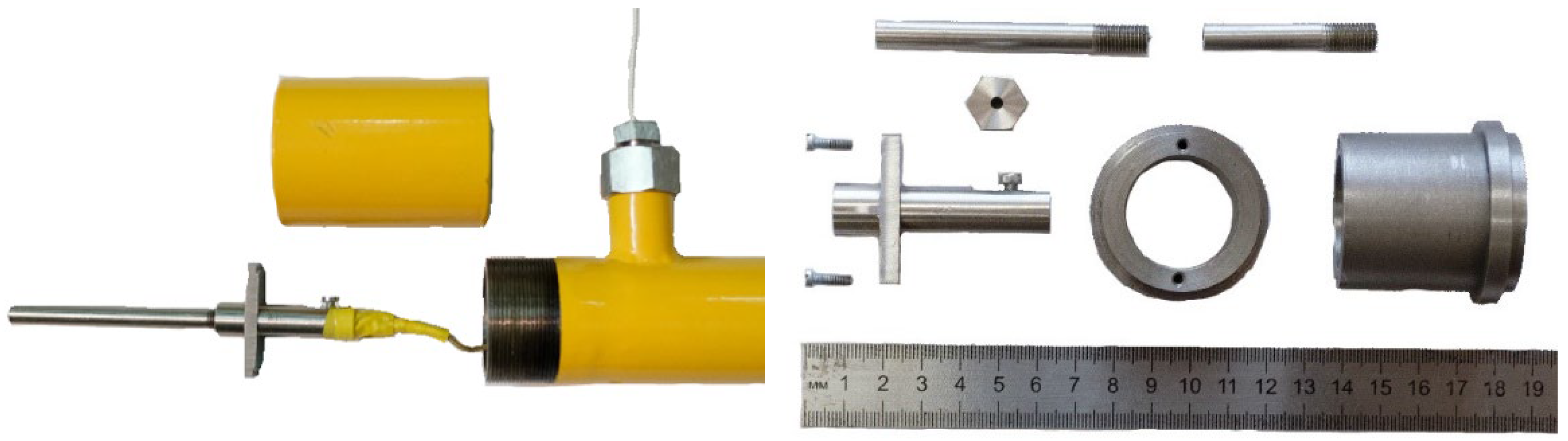
To study the Hartmann–Sprenger effect, an experimental setup (Figure 4) operating in dry air was designed and constructed. Its design allowed for the interchangeability of nozzle devices (Figure 5) and resonators (Figure 6), as well as adjustments to the distance between the nozzle and the resonator using a threaded connection between two parts of the housing. The dimensions of the setup were calculated based on the pressure produced by the compressor used in the experiment.

A Laval nozzle was used as a booster (Figure 5), the geometry of which was calculated using a standard technique for a dry air flow rate of 60 nm³/h, an inlet overpressure of 0.6 MPa, and an outlet pressure of 0 MPa, with an inlet air temperature of 20 °C. To compare it with the traditional reduction case, a replaceable throttle with a hole diameter equal to the nozzle throat diameter of 3 mm was used.

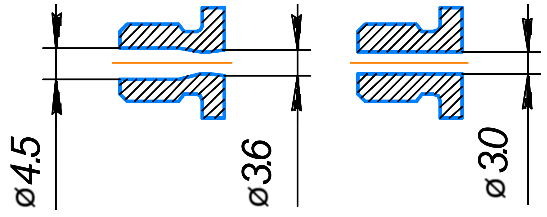
Based on the recommendations of various authors, which will be described below, the following characteristics were adopted for the three cylindrical resonators (Figure 6): the inner diameter and wall thickness of all three were 4.2 mm and 1.9 mm, respectively; and the inner lengths were 45.5 mm for the small resonator, 70.5 mm for the medium resonator, and 97.5 mm for the long resonator.

To measure the air temperature inside the resonator, a 1 mm diameter hole was made in its bottom to divert part of the heated air to a thermocouple. This approach reduced the efficiency of the heating of the volume of gas trapped inside the cavity but allowed for more precise temperature measurements.

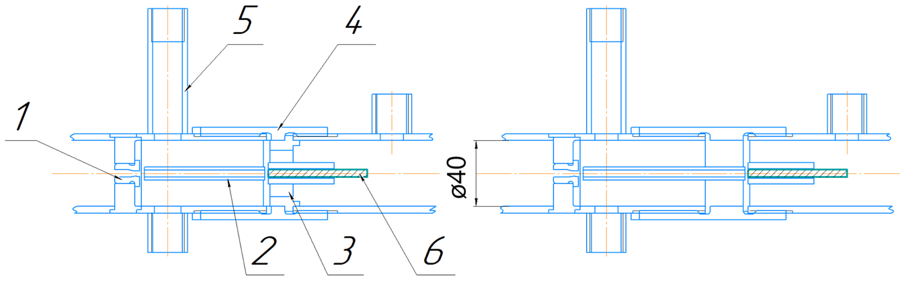
The distance from the nozzle discharge edge to the input resonator was adjusted by rotating the right side of the housing (Figure 7) relative to the left side. In this case, the base (3) of the resonator (2) was fixed on the right side of the device using the sleeve (4). Figure 6 does not show the option for mounting the third “small” resonator, as its base shares a common base with the medium resonator (Figure 8).

Figure 8 shows the bases of various resonators, which are secured by sleeves to the rotating right part of the housing.

The material of the structural elements of the installation was Steel 3, while the material of the nozzle, throttle, and resonators was steel 12Kh18N10T.

The equipment used in the experiments is presented in

Table 1. Characteristics of the setup elements and measuring instruments.

No.	Type	Title	Characteristics
1.	Compressor with low temperature dryer	Fini Plus 8-08-270 ES (FNA S.p.A., Robassomero, Italy)	Screw type. Receiver 270 l.
2.	OVEN (OVEN Ltd., Moscow, Russia) pressure transducers	PD100-DI1.0-111-0.5 PD100-DI0.4-111-0.5	Measurement ranges of 0 … 1.0 MPa and 0 … 0.4 MPa. Basic reduced error, ±5 kPa and ±2 kPa, respectively.
3.	OVEN (OVEN Ltd., Moscow, Russia) thermal resistance sensors	DTS335-50P.V3.60 DTS014-RT100.V3.20/1.5	The measuring range is −196 … + 660 °C and −60 … + 250 °C. The limit of permissible deviation is ±(0.30 + 0.005 ∙ t) °C. Thermal inertia is no more than 10 … 30 s. Three-wire connection diagram.
4.	OVEN (OVEN Ltd., Moscow, Russia) open-frame thermocouple	DTPK031-0.5/0.05/1.5	The measurement range is −40 … + 1100 °C. The tolerance limit is ±2.5 °C. Thermal inertia is no more than 3 s.
5.	OVEN (OVEN Ltd., Moscow, Russia) analog input module with fast inputs	MV110-224.8A	RS-485 interface. The inquiry time of one input is not more than 5 ms ± 2%.
6.	Noise and vibration analyzer	Svan 912M (SVANTEK Sp. z o.o., Warsaw, Poland)	The measurement range is 21 … 140 dBA. The total error is less than 0.7 dB.

. Data from the sensors were visualized and stored using the Trace Mode 6 SCADA system (AdAstra Research Group Ltd., Moscow, Russia).

Before starting experiments on the generation of characteristic sounds and the increase in temperature for each resonator, the working ranges of distances from the trailing edge of the nozzle to their inlets were determined. In Figure 4, the long wires from the temperature sensors can be seen. After determining the operating range, these were replaced with short wires of uniform length (70 cm) to improve accuracy.

The inlet pressure was maintained at the calculated level using inlet valve 2 (Figure 4). Air was supplied to the unit from the receiver through the dryer, with the compressor inactive. It should be noted that, due to the limitations of the receiver, long-duration tests were not conducted. In each experiment, the nozzle operated in the calculated mode for about 25 to 30 s. As a result, due to the high heat capacity of the resonator base and thermal inertia, heat transfer from the heated gas to the flow passing through the resonator made it difficult to estimate the temperature at the outlet of the device. Nevertheless, each experiment was carried out for a longer period (up to 2 min) until, due to the pressure drop, the temperature at the bottom of the resonator began to drop sharply.

The frequency of the characteristic sound was measured for various resonators. The measurements were taken without the use of a muffler at the outlet of the setup, which was used in the subsequent experiments due to the excessive noise level. The additional back-pressure from the muffler was accounted for when processing the results.

The temperature and pressure values were measured at the device inlet, before the nozzle, and at the outlet using pressure and temperature sensors 5 and 6.

Since the primary parameter of interest was temperature, the experiments were organized and the statistical processing of their results was conducted with a focus on temperature measurements.

For the confidence level $\alpha =0.05$, the number of measurements at each distance for each resonator (measurement series) was determined based on the dispersion $S^2$ and the total measurement error ${\delta }_{\mathsf{\Sigma }}$, calculated from the data of preliminary experiments:

$$n\ge {\displaystyle \frac{t_{\mathrm{\infty },\alpha /2}^2{S}^2}{{\delta }_{\mathrm{x}}^2}}=5,$$

(4)

where $t_{\infty ,\alpha /2}$ is Student’s test value for the number of degrees of freedom $f=\infty$ and the confidence level $\alpha$, taking into account two-sided restrictions.

For each measurement series $i$, the variance was calculated:

$$S_i^2={\displaystyle \frac{1}{n-1}}\sum {\left(x_j-{\overline{x}}_j\right)}^2,$$

(5)

where $n_i$ is the number of measurements in the series; and $x_j$ and ${\overline{x}}_j$ are the measured and arithmetic means of the desired quantity in the series, respectively.

The weighted average over all series of experiments was obtained as follows:

$$S_w^2={\displaystyle \frac{\sum f_i{S}_i^2}{\sum f_i}},$$

(6)

where $f_i=n_i-1$ is the degree of freedom of each series of measurements.

The absolute random error was determined:

$${\delta }_r=\pm {\displaystyle \frac{t_{f,\alpha }{S}_w}{\sqrt{n_i}}},$$

(7)

where $S_w$ is the mean standard deviation weight-averaged over all series.

The total absolute error of the direct measurement $x$ was calculated, taking into account the random and instrumental errors:

$${\delta }_x=\pm \sqrt{{\delta }_r^2+{\left({\displaystyle \frac{K_{\alpha }}{3}}\right)}^2{\mathsf{\Delta }}^2},$$

(8)

where $\mathsf{\Delta }$ is the absolute instrumental error (Table 1); and $K_{\alpha }\approx t_{\infty ,\alpha }$ is the safety factor.

For indirect measurements of a complex quantity $y=f\left(x,z\right)$, the total error was calculated, taking into account the total errors of several directly measured quantities $x$ and $z$:

$${\delta }_y=\pm \sqrt{{\left({\displaystyle \frac{\partial y}{\partial x}}\right)}^2{\delta }_x^2+{\left({\displaystyle \frac{\partial y}{\partial z}}\right)}^2{\delta }_z^2}.$$

(9)

When determining the temperature exceedance inside the resonators relative to the input temperature, the total error was 2.47 K. The difference between the output and input temperatures was 0.59 K. The temperature growth rate inside the resonators was 2.99 K. The duration of the self-sustaining effect at the level of 95% of the maximum temperature had a total error of 0.04 s. The range of inlet pressures that ensured the self-sustaining effect at the level of 95% of the maximum temperature had an error of 3.45 kPa.

Since it is difficult to experimentally determine the temperature and velocity of the incoming flow, the temperature of adiabatic deceleration was calculated based on the simulation results, assuming that the heat capacity of the air remained unchanged, using the following relation:

$$T_t=T_f+{\displaystyle \frac{w^2}{2c_p}}=T_f\left(1+{\displaystyle \frac{k-1}{2}}{M}^2\right)=T_f+{\displaystyle \frac{k-1}{2kR}}{w}^2=319.21\mathrm{K},$$

(10)

where $T_f=218 \mathrm{K}$ is the incident flow temperature; $k=1.4$ is the adiabatic index; $R=287.1$ J/(kg ∙ K) is the individual gas constant; $w=$ 451 m/s is the flow rate; and M is the Mach number.

5. Experimental Results

The environment temperature during the experiments was approximately 27 °C, while the temperature at the nozzle was 25 °C.

Initially, the working ranges of the distances $l$ between the nozzle and the inlet of the resonators were set as follows: 6.0 mm … 9.5 mm (relative to the nozzle critical section diameter $d$: 2.00 … 3.17) for the 45.5 mm resonator, 5.5 mm … 10.5 mm ($l/d$ = 1.83 … 3.50) for the 70.5 mm, and 6.5 mm … 12.0 mm ($l/d$ = 2.17 … 4.00) for the 97.5 mm resonator. These ranges of distances were where the graphical dependencies were presented. The longer cavities had a wider operating distance range, which extended farther from the nozzle exit. This may be due to the fact that, in order to complete the full cycle of the effect, a larger volume of gas must be evacuated from a longer resonator, which results in less resistance from the jet.

The highest temperatures at the bottom of the resonator (Figure 9), minus the temperature in front of the nozzle, were achieved with the longest resonator cavity (97.5 mm). This allowed the heated gas to remain longer in the dead-end region, cumulatively receiving new portions of energy. The maximum excess temperature over the one in front of the nozzle was 102 K for the 97.5 mm resonator, 79 K for the 70.5 mm resonator, and 78 K for the 45.5 mm resonator. At all distances from the nozzle to the resonator, the temperatures in the dead-end region of the resonator were higher than the stagnation temperature, the level of which is shown in Figure 9 for a correct comparison, minus the temperature in front of the nozzle.

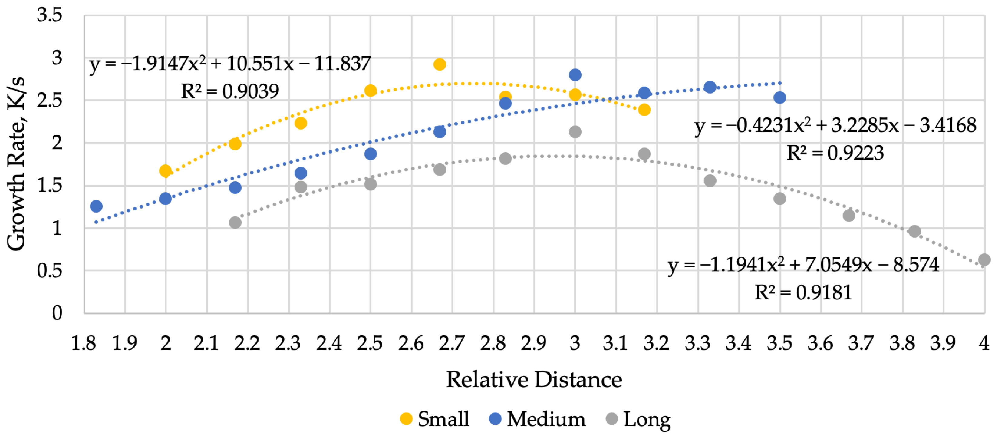
The average growth rates were 1.43 K/s for the 97.5 mm resonator, 2.07 K/s for the 70.5 mm resonator, and 2.36 K/s for the 45.5 mm resonator. The highest growth rates of the gas temperature in the resonator cavities (Figure 10) were achieved with shorter resonator lengths, which was explained by an increase in the frequency of pressure fluctuations as the wave path length decreased.

The largest temperature increase, as well as the highest growth rates, were observed at approximately the same distance from the nozzle to the resonator: 8.5 … 9.0 mm ($l/d$ = 2.83 … 3.00). This corresponded to the location of the instability zone immediately in front of the resonator inlet.

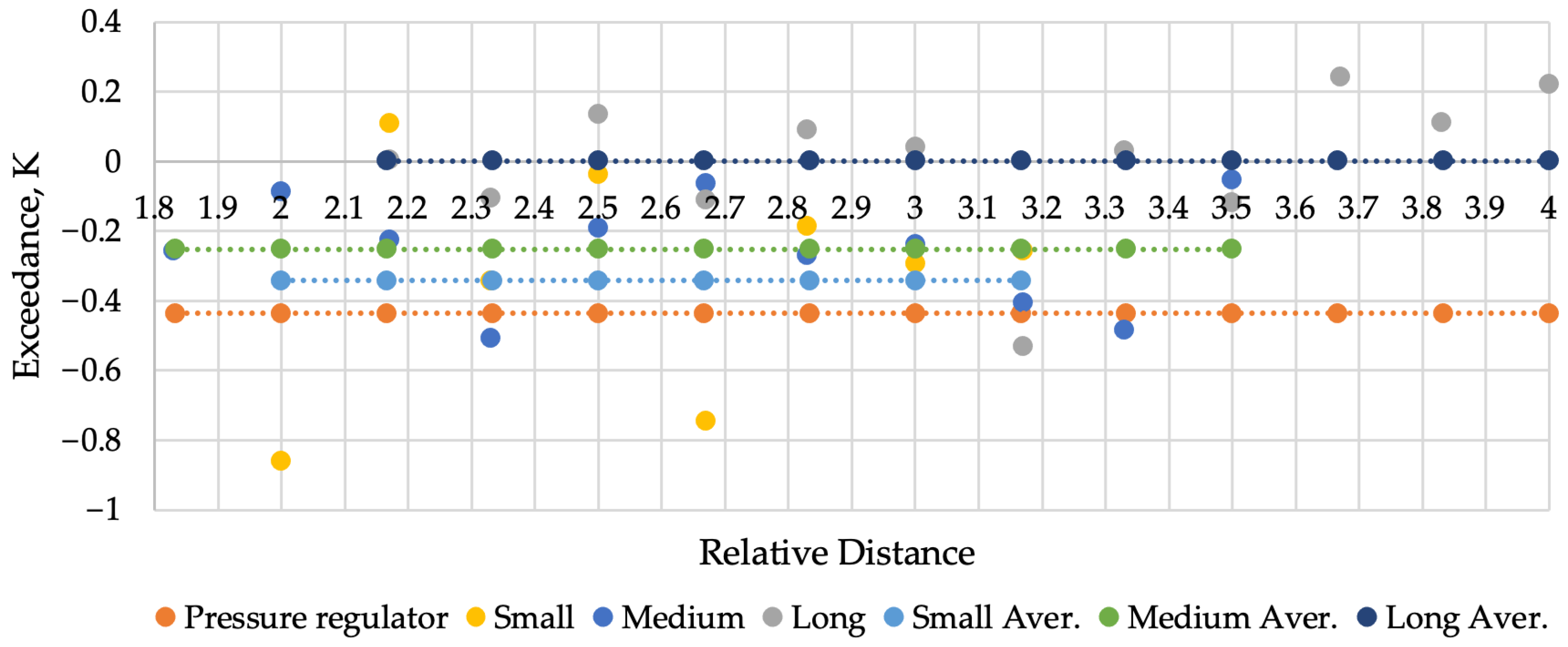
In a pilot installation, when using all three resonators, throttling with the Hartmann–Sprenger effect resulted in an average outlet temperature higher than when throttling through a hole (Figure 11). The best performance was demonstrated by the long resonator. However, despite the observed qualitative trend, the quantitative values cannot be considered statistically significant due to the small magnitude of the sought-for values and high errors. Additionally, it is important to note the differing thermal inertia during heat transfer through the resonator walls, which is attributed to the variations in the mass of the metal in their mounting bases. The long resonator had the smallest mass for the additional base, while the small resonator had the largest.

During the experiments, it was observed that in the first half of the working distance ranges between the nozzle and resonators, the stable existence of the Hartmann–Sprenger effect lasted longer (Figure 12) and over larger ranges of pressure drop across the nozzle (Figure 13). In terms of time, it lasted longer on average: 2.13 times longer for the 97.5 mm resonator, 2.35 times for the 70.5 mm resonator, and 1.58 times for the 45.5 mm resonator. The pressure drop range was larger on average: 4.37 times larger for the 97.5 mm resonator, 2.78 times for the 70.5 mm resonator, and 1.87 times for the 45.5 mm resonator.

It is interesting to note that the inflection point of the curves corresponds exactly to the distance between the nozzle and the resonator, which aligns with the maximum temperatures and their growth rates. This is likely due to the fact that as the distance decreased, the instability zone remained in front of the resonator inlet due to its length. However, as the distance increased, the level of non-stationarity at the inlet dropped sharply, as confirmed by mathematical modeling conducted in a previous study [38].

The best results, averaged over distance ranges for durations and pressure drop ranges within which the Hartmann–Sprenger effect was stably maintained, were demonstrated by the medium resonator (70.5 mm). The results for the small resonator (45.5 mm) were similar. The worst results were observed for the long resonator (97.5 mm). This was likely due to the position of the long resonator being farther from the nozzle, which, with a decrease in pressure drop, caused a more significant reduction in the energy of the jet in front of the resonator.

The resonant frequencies of sound oscillations were determined for each resonator length: 764 Hz for the 97.5 mm resonator, 1055 Hz for the 70.5 mm resonator, and 1656 Hz for the 45.5 mm resonator.

The frequency of natural oscillations was twice as high as the resonance frequency, as the wave changed sign when reflected from the open end. Instead of the reflected shock wave, a rarefaction wave passed through the pipe. Based on this, the natural frequencies of the resonators were 1528 Hz for the 97.5 mm resonator, 2110 Hz for the 70.5 mm resonator, and 3312 Hz for the 45.5 mm resonator.

Despite the relatively low air flow rate and pressure drop, the noise level exceeded the 55 dB limit for human hearing. However, the frequency measurements were taken without sound insulation. In actual operation, the process will occur inside the pipeline, which will significantly reduce the sound impact, while the impact of vibrations will become more relevant. The main results of the experiments are presented in

Table 2. Main results.

Type of the Resonator	Maximum Heating, K	Temperature Growth Rate, K/s	Resonant Frequencies, Hz
Short resonator	78	2.36	1656
Medium resonator	79	2.07	1055
Long resonator	102	1.43	764

.

6. Average Marginal Cost of the Device

Since there are currently no market analogs in terms of design, the marginal cost of the pressure regulator was determined. This helped to identify specific design solutions that could be developed to make the product economically efficient.

The calculation was performed based on the assumption that installing one device at each of the 3800 gas distribution stations of PJSC Gazprom would save 30% of annual fuel gas consumption. Additionally, it was assumed that all stations had the same hourly commercial consumption of natural gas of approximately 7000 m³/h.

The cost of gas for internal use was assumed to be $50 per unit. The 30% savings assumption was based on the experience of operating reducing devices using the Ranque–Hilsch effect, which has shown sufficient efficiency during the spring–summer period.

The average marginal cost of one device was equal to 30% of the annual fuel gas expenditure divided by the number of stations. The time factor was not considered in this calculation.

The calculation of the average marginal cost of the device is presented in

Table 3. Calculation of the average marginal cost of the device.

Name of Indicator	Unit of Measurement	Value of Indicator	Remark
Amount of gas for own needs for heaters	million m3/year	809.6	According to gas consumption data of heaters from Gazprommash Plant LLC (St. Petersburg, Russia)
Share of the fuel gas saving	%	30	Based on expert assessments
Value of the fuel gas saving	million m3/year	242.9
The cost of natural gas for own needs	USD/thousand m3	50	According to LLC Gazprom Transgaz St. Petersburg, Russia
Potential savings for gas transport companies	thousand USD/year	11,389.23
Average marginal cost	thousand USD/piece	2.99

. The marginal cost of one pressure regulator was found to be USD 2.99 thousand.

7. Discussion

Based on an experimental comparison of three resonator lengths, the following conclusions were drawn:

• Small resonators should be used to achieve maximum temperature growth rates, as the frequency of pressure fluctuations increases with a shorter wave path.
• Long resonators should be used to achieve maximum temperatures, as their length allows the heated gas to remain for longer in the dead-end region, cumulatively receiving more energy.
• The medium resonator demonstrates the best reliability under non-stationary power conditions, while the small resonator shows similar results.
• The worst performance is observed with the long resonator, due to its greater distance from the nozzle. As the pressure drop decreases, this leads to a more significant loss of jet energy before reaching the resonator.

This study emphasized the importance of proper resonator placement relative to the nozzle. It demonstrated that as the distance decreased, the instability zone remained in front of the resonator inlet due to its length. However, as the resonator moved farther away, the level of non-stationarity at the inlet dropped sharply. This finding aligns with the results of the mathematical modeling conducted in the previous study [39].

The maximum-achieved heating was 102 K, and the maximum temperature growth rate was 102 K/s. These results were significantly lower than those reported by other researchers, who achieved temperatures up to 1600 K [40] and heating rates up to 160 K/ms [41]. This discrepancy can be attributed to technical constraints, such as the low pressure and low flow rate. Future research will include experiments under industrial pressure and gas flow conditions.

The results closest to isothermal reduction were achieved by the long resonator. In general, the comparison with throttling, along with results from external sources, demonstrated the potential for using the Hartmann–Sprenger effect in pressure reduction. The significance (efficiency) of this effect will depend on the power supply conditions of the installation and, consequently, the size of the reduction point. In this study, the experiments were conducted for a case where the Hartmann–Sprenger effect functioned in regurgitation mode, with low flow rates and pressure drops typical of small reduction points. The effectiveness of applying the Hartmann–Sprenger effect in such technological chains was not as pronounced, and it was likely not economically viable, as the negative cooling effect of throttling was less significant. However, in large gas-reducing facilities, where the high negative effect of throttling necessitates the use of burner heaters for the reduced gas, the benefits of applying the Hartmann–Sprenger effect will be significant.

The experiments were conducted using dry air. In industrial applications, pressure regulators are typically located at gas distribution stations, positioned “at the other end” of the pipeline network, following a series of cleaners and dryers at compressor stations. Similarly, at gas distribution stations, they are positioned after the filters. However, the transported gas may contain moisture and other impurities, which could affect the performance of the Hartmann–Sprenger effect. This issue was not examined in detail in this paper but will be addressed more thoroughly in future research.

The calculated average marginal cost of a pressure regulator based on the Hartmann–Sprenger effect was approximately 3.5 times higher than that of traditional pressure regulators. While this was a significant difference, it remained a relatively good result, as there was room for the cost of the structure to rise.

8. Conclusions

The results of this study indicate that small resonators should be used to achieve the highest temperature growth rates, long resonators to achieve maximum temperatures, and medium resonators for the best reliability under non-stationary conditions. In general, the highest reliability is observed in the first half of the range of distances between the nozzle and the resonator, regardless of the resonator length. Reliability is the most critical property for natural gas transportation and distribution systems.

The results of the conducted studies demonstrate the feasibility of implementing a quasi-isothermal natural gas pressure regulator based on the Hartmann–Sprenger effect. The acquired data show sufficient performance over a fairly wide range of distances from the nozzle to the resonator. Noise and vibrations remain within acceptable levels for technological equipment. A pressure regulator based on the Hartmann–Sprenger effect has the potential to be economically viable.

This work explores the possibility of using the effect for a specific practical application, which is characterized by both technological limitations, such as the non-uniformity of gas flow and variations in pressure drop, and geometric constraints, such as the need to fit within the installation dimensions of traditional pressure regulators. To verify the feasibility of using the effect in a real system with changing conditions, it is important to consider all characteristics in an integrated manner: the maximum temperature for economic efficiency, the heat rate and stability of effect maintenance for operation under non-stationary conditions, and the mutual geometrical dimensions of the nozzle, resonator, and their distance, which ensure effective operation. It is also necessary to allow for their relative movement and, in general, to consider the geometric dimensions of the potential device to ensure proper installation.

Approaches based solely on theoretical justifications or selective characteristics (such as maximum temperature), as covered in other articles, are incomplete, as they do not provide a comprehensive understanding of the effect’s potential, not just for pressure reduction but also for pressure regulation (i.e., reducing and maintaining pressure at a given level under varying supply conditions).

For this reason, further experiments are required to develop the topic and evaluate the device’s effectiveness. Since the experiments are conducted at low pressures due to technical limitations, it is crucial to test the device under real flow and pressure conditions at large pressure reduction facilities. Additionally, the device’s performance must be evaluated in screech mode. These additional tests will help determine the economic feasibility of this study.