Article

Investigation of Surface Quality and Productivity in Precision Hard Turning of AISI 4340 Steel Using Integrated Approach of ML-MOORA-PSO

1
Department of Mechanical Engineering, College of Engineering, King Saud University, P.O. Box 800, Riyadh 11421, Saudi Arabia
2
Production Engineering Department, National Institute of Technology Agartala, Jirania 799046, India
3
Department of Mechanical Engineering, Southern Methodist University, 6425 Boaz Lane, Dallas, TX 75205, USA
4
Department of Mechanical Engineering, Graphic Era (Deemed to be University), Dehradun 248002, India
5
Department of Mechanical Engineering, The British University in Egypt, El-Sherouk City, Cairo 11837, Egypt
*
Author to whom correspondence should be addressed.
Processes 2025, 13(4), 1156; https://doi.org/10.3390/pr13041156
Submission received: 25 February 2025 / Revised: 27 March 2025 / Accepted: 2 April 2025 / Published: 10 April 2025

Abstract

:
AISI 4340 steel has applications in gun barrels, where the surface quality of the barrel is the prime factor. This study explores the application of a machine learning (ML) approach to optimize the precision turning of an AISI 4340 steel alloy using both conventional and wiper tool nose inserts under varying cutting parameters, such as cutting speed, depth of cut, and feed rate. The analytical framework integrates experimental machining data with computational algorithms to predict key output parameters: surface roughness (Ra) and material removal rate (MRR). A Multi-Objective Optimization based on Ratio Analysis (MOORA) method is used for data normalization. Particle swarm optimization (PSO) further refines the process by optimizing the input parameters to achieve superior machining performance. Results show that under optimized conditions, a 118 m/min cutting speed, 0.22 mm depth of cut, and 0.2 mm/rev feed, wiper inserts provide a 50% improvement in Ra compared to conventional inserts, highlighting their potential for enhancing both productivity and efficiency. At the suggested setting, the surface roughness values are 0.59 µm for wiper inserts and 1.30 µm for conventional inserts, with a material removal rate of 4996.96 mm3/min. The developed empirical model serves as a powerful tool for improving precision hard-turning processes across manufacturing sectors. The present work employs the XGBoost model of ML along with MOORA and PSO to predict and optimize machining outcomes, advancing hard-turning practices by delivering quantifiable improvements in surface quality, material removal rate, and operational efficiency.

1. Introduction

The precise turning of high-strength materials means the turning of materials with high hardness, high wear resistance, better mechanical characteristics, etc., such as titanium alloy, nickel-based superalloys, and alloy steel. These materials have different advanced applications [1,2,3,4,5] but are categorized as hard to machine due to low thermal conductivity and high specific cutting energy. Therefore, advanced machining methods are considered the optimal machining technique to process alloy steel [6,7]. Due to the high cost of machining associated with non-traditional machining methods, conventional machining methods are considered over them [8]. Initially, it was considered that grinding was the only method (except non-conventional) to process these hard-to-machine materials. However, there is a growing demand for new conventional methods to machine alloy steel due to the limitations of geometry-related tasks and the flexibility of the process. Hard turning is one of the processes to machine the alloy steel, which can reduce the processing time by 60%. The prime feature of hard turning is the precise production of complex shapes with great tolerance [9]. Hard turning can process the hard-to-machine materials easily with a high material removal rate and good surface quality. Due to this characteristic, hard turning has several applications in industries varying from automobiles to spacecraft. Due to precise machining characteristics, hard turning has applications in sensors, laser scanners, microelectronics, telecommunication, etc. [10]. Another application of precision hard turning is observed where a high amount of precision is required like jigs, cutting tools, etc. The components developed from steel alloys exhibit high wear resistance, high fracture toughness, high strength, and high hardness. AISI 4340 is also a category of steel alloy, which represents good mechanical characteristics. Due to better mechanical characteristics, these alloys have applications in the defense sector, power generation, construction, automobile, etc. [11,12,13].
Steel alloys are categorized as hard-to-machine alloys due to their high strength. The strength of these steel alloys is sufficient to cause the cutting tools used for the processing of these alloys. Many methods are adopted to machine the steel alloys, which include conventional machining (dry machining, machining with lubrication) and non-conventional machining. In dry machining, coated and uncoated inserts of different materials were used [14,15,16,17,18]. However, in the machining with the lubrication, various types of lubrications were used including flood lubrication, minimum quantity lubrication, solid lubrication, etc. [19,20,21]. Flood machining is not an economical way of machining. From the reports, it is calculated that the annual cost of lubricants used in conventional machining (in the USA alone) is more than USD 100 billion. The lubricant cost in machining varies from 7% to 17% of the total machining cost. Therefore, subtracting the lubricant in the machining process reduces the overall cost of machining [22,23,24]. In dry machining, the lubricant is eliminated, which reduces the cost of machining as well as the fumes generated (during the burning of lubricant). Dry machining may be considered a step towards a sustainable approach because (i) the lubricant is eliminated, which makes the process economical; (ii) the health hazards of operators are reduced, which are increased during the burning of lubricant; and (iii) the chances of environmental pollution of are reduced as after the lubricant’s life is over, it is disposed of, which causes soil contamination [25,26,27,28,29]. Dry machining is also known as green machining, as it is safe for the operator as well as the environment. In the case of hard-to-machine materials, the coated tool inserts are used with different materials like tungsten carbide, cubic boron nitride, etc.
Steel alloys are assumed to exhibit low machinability due to large strength and low ductility. On the other hand, the demand for alloy steels in industries is increasing day by day. Due to this, the processing of alloy steel became a challenging task for manufacturing engineers [14]. In the current work, an attempt has been made to process the alloy steel 4340 using different types of tool inserts and investigate response variables considering the quality and productivity of the product. Therefore, material removal rate (productivity) and surface roughness (quality) are considered as the response variables. Researchers used different types of tooling like ultrasonic-assisted, magnetic field-assisted, laser-assisted, uncoated, textured tool inserts, and tool inserts with micro-channels [16,17,19]. Wiper-type inserts, although relatively new, have shown great promise. Unlike conventional inserts, wiper geometry tool inserts have a series of radii, due to which precise hard turning of hard-to-machine materials can be possible. Despite the increasing popularity of wiper inserts, limited research has been conducted on their performance, particularly in combination with machine learning (ML) techniques for optimization, which presents a key novelty in this work. The use of the ML approach, especially the XGBoost model, is justified only because of its characteristic ability to provide robust predictions and non-linear relationships [30]. These models are capable of capturing complex data from the experimental values, which is a challenging task for statistical techniques. The regularization capabilities of the XGBoost model reduce the overfitting along with the enhancement of prediction accuracy, which makes them fit for the optimization of machining parameters. Previous work is described in the paragraph below.
Charalampous [31] investigated the cutting forces using the ML approach while processing the AISI 4140 steel alloy. Initially, experiments were performed as per the experimental set, and the prediction of results was made using the ML approach. The model was adapted to predict the tool wear while conducting machining operations. In another study conducted by Dubey et al. [32], the machining of SS304 was performed in the presence of particles with minimum quantity lubrication (MQL) and the surface roughness was evaluated using three different approaches of ML (linear regression, random forest, and support vector machine). In their research, the random forest approach outperformed the other two approaches. The particle size of 30 nm provides a better R-square value compared to other particle sizes. Korkmaz et al. [33] worked on Bohler steel and investigated tool wear in the case of minimum quantity lubrication. It has been found that the flank wear is reduced by 5%, 10%, and 25% when MQL is applied on the flank face, rake face, and both faces. Ross et al. [34] machined AM 316 steel alloy using different deep-learning models to investigate the surface roughness of the machined surface. Researchers processed a SS316 alloy using different cooling conditions like dry, MQL, CO2, and CO2 + MQL. Hybrid cooling was observed to be the best cooling method compared to others and reduced the surface roughness by 52–56%.
In the field of advanced manufacturing, precision, surface roughness, and efficiency are paramount. From intricate mechanical components to complex assemblies, Computer Numerical Control (CNC) machining plays a vital role in transforming digital designs into tangible realities. It is a well-known fact that the surface created during turning depends upon the nose radius of the tool, feed, depth of cut, material of tool inserts, etc. Tool inserts with round geometry (nose) limit the production rate due to the upper feed rate limit restrictions [31]. The research conducted by Gao et al. [32] created a prediction model for the surface roughness of precision grinding. The prediction errors for surface roughness and sub-surface damage depth by the predictive models are 6.3% and 6.9%, respectively. This productivity can be improved after incorporating a wiper geometry, which is capable of achieving higher feed values compared to conventional tool inserts. At the same time, the quality of the machined surface is better than the machined surface obtained by conventional tool inserts [33,34]. This study stands out by demonstrating the significant benefits of wiper geometry in hard turning, particularly through the integration of machine learning and optimization techniques such as the MOORA method and PSO, which are underexplored in the existing literature. In the previously published research, it has been identified that the use of wiper geometry tool inserts increases the MRR and surface quality, but the power consumption and cutting force were also increased [8,35]. Due to the increase in the temperature at the rake face of the tool inserts, the residual stresses on the machined surface were also increased [36].
The AISI 4340 steel alloy has applications in gun barrels, gears, or bearings. These applications are in fields where a sliding or rotating contact often occurs. Therefore, low surface roughness is essential to minimize friction, wear, and potential damage. By achieving the desired surface roughness, we can ensure that the component functions optimally and meets the design requirements (Ra ≤ 0.8 µm). Surface roughness also influences the fatigue strength and durability of components. High surface roughness can act as a stress concentrator, leading to the initiation and propagation of cracks under cyclic loading conditions. By minimizing the surface roughness, a reduction in stress concentration along with improvement in the fatigue life and durability of the machined parts can be achieved, making the product more resistant to failure. The researchers worked on similar materials [37,38] and found that signals are 74% effective for flank wear with the help of sensor fusion by tool condition monitoring.
Several researchers used different optimization techniques for the parametric optimization of precise machining, which includes response surface methodology, genetic algorithm, non-dominated sorting genetic algorithm-II, artificial neural networks, teaching learning-based optimization, etc. [4,39,40,41,42]. However, limited research has focused on integrating machine learning with optimization techniques for the hard turning of AISI 4340 steel, especially using wiper geometry. This work addresses that gap by developing an empirical model, applying the MOORA method for normalization, and using particle swarm optimization (PSO) to optimize machining parameters. This integrated approach provides a novel contribution to the optimization of precision hard-turning processes. In the current research, the results of a previously conducted full factorial experimental plan [41,43] have been further examined. The novelty of this research lies in the integration of the XGBoost machine learning model with MOORA and PSO for optimizing the precision turning process of AISI 4340 steel. Unlike previous studies, which often focus on either empirical modeling or traditional optimization methods, this work leverages advanced computational techniques to enhance predictive accuracy and optimization efficiency. The combined approach not only improves surface quality and material removal rate but also provides a robust decision-making framework for machining applications, particularly in high-precision industries such as firearm manufacturing. The objectives of the present research are as follows:
(i)
To look deeper into the influence of wiper geometry and conventional tool inserts on productivity (MRR) and quality (Ra).
(ii)
To predict the Ra (after machining by wiper and conventional tool inserts) and MRR after implementation of the ML approach. The results obtained after the above-mentioned approaches will be compared to find the best one, which will be more suitable to adopt the design parameters of for the application of gun barrels.
(iii)
To convert the predicted solutions into a single dimensionless quantity known as a performance measure (PM) after normalization using the MOORA method.
(iv)
To develop the empirical model for PM and set up a relation between the input parameters and PM.
(v)
To apply the PSO on PM for the optimization of input parameters and perform the validation experiments at the suggested setting. Compare the results of the hybrid approach ML-MOORA-PSO with the ML-MOORA.

2. Materials and Methods

This paper provides a comprehensive analysis of experimental studies previously conducted on AISI 4340 alloy steel, as detailed in Refs. [41,42]. The mechanical characteristics and chemical composition of the material used are published by Abbas et al. [41]. A concise overview of the experimental work reported by Abbas et al. [41], as follows.

2.1. Test Specimen and Cutting Tool Specification

A cylindrical bar of 60 mm diameter and 130 mm length was used for the experiment [41]. In each sample, a 15 mm length was machined with a 5 mm clearance. The process flow adopted in the current work is shown in Figure 1. The CNC lathe used for the tests was an EMCO (Hallein, Austria) Concept Turn 450 equipped with a Siemens Sinumeric 840D. Precision hard turning of the steel alloy was performed using Sandvik (Sandviken, Sweden) conventional (DCMT11T304-PF) and wiper geometry (DCMX11T304-WF) tool inserts. These inserts had rake angles of 6° and 18°, respectively. Both inserts shared identical cutting-edge angles (55°), clearance angles (7°), and nose radii (0.4 mm). A tool holder with specification SDJCL 2020K11 (Sandvik, Sweden) was used to secure both types of inserts.

2.2. Surface Roughness Evaluation

A TESA-Rugosurf 90G surface roughness tester (Renens, Switzerland) was used to find the grade of roughness after each test. The parameters of measuring set for the measurement of surface roughness were as follows: cut of length 0.8 mm, cut-off number 10, measuring speed 1 mm/s, and curved measurement surface. The test rig for measuring the surface roughness is shown in Figure 1. Each measurement was repeated three times on a particular surface and after that, the average of three values was selected for analysis purposes. The accuracy of the reading is 0.02 microns.

2.3. Experiments Configuration

A full factorial design of experiments was employed, considering three input parameters—cutting speed, depth of cut (DoC), and feed rate (f)—each at four levels (Table 1). This resulted in a total of 64 experimental runs. The experimental design matrix and the corresponding results are detailed in Appendix A Table A1. These parameters were selected after consulting with the Sandwik expert and Industry engineers. Turning operations were conducted using two distinct insert types: wiper geometry and conventional. Consequently, a total of 128 experiments were performed on AISI 4340 alloy steel. A coolant consisting of ECO-COOL-MK-3 mixed with distilled water was used throughout the study.

2.4. Methodology

In the present work, an integrated approach has been used for the processing of input parameters and results obtained. Initially, the full factorial design was used for the planning of experiments. After that, the solutions are predicted using a machine-learning approach. The approach exhibits minimum error, which was used for further analysis. Therefore, the MOORA method was used for the ranking of solutions predicted by the ML approach. After that, PSO was used for the optimization of solutions, and finally, confirmation experiments were performed to check the suitability of the proposed approach. The main reason for adopting the integrated approach of ML-MOORA-PSO is the out-performance of the specified method over the current approach. The ML approach is used instead of other techniques, viz. neural networks or regression-based models, because it captures the complex non-linear relationship in the machining process along with the efficient prediction in turning process optimization. The advantages of using XGBoost over other methods are higher accuracy and generalization ability, better performance on tabular data, lower computational cost as compared to NN, and handling capability of missing and noisy data. After obtaining the predicted values, the MOORA is chosen as the MCDM method because it can handle multi-objective problems. The main advantage of MOORA over TOPSIS and AHP is the straightforward ratio, which is computationally less intensive. The decision-making is better in conflicting nature objectives by the MOORA method, which effectively ranks alternatives without being sensitive to the weight assignment issues that affect TOPSIS. The stability and robustness are good, and it avoids the rank reversal issue and hence depicts consistent results. The use of PSO over other metaheuristic algorithms is due to its fast convergence speed and efficient search in complex spaces. Thus, PSO efficiently searches for optimal solutions by dynamically adjusting the positions of candidate solutions in the search space. The code is developed using MATLAB (R2017a version 9.2). It is a custom-developed script utilizing built-in MATLAB functions and user-defined functions.

2.4.1. Machine Learning (ML) Methodology

In the current research, the XGBoost model of the ML approach was used for the prediction of Ra and MRR for AISI 4340 steel. The R 4.3.0 software was used for the implementation of the ML approach. The proposed model was used to obtain robust predictions and assess their suitability for the optimization of process parameters of the machining process. The details regarding the data preparation, model training and evaluation are given below.
Data Preparation: In data preparation, the first step is to prepare the dataset. In this, the input parameters like CS, DoC, and f and output parameters like Ra and MRR are compiled. Of the data, 70% were used for training purposes and 30% for testing. The second step is feature engineering, in which all the input (independent) variables are converted into a matrix using the ‘as.matrix ()’ function in R. The output (or target or dependent) variables were isolated as numeric arrays. The third step is normalization, which was used for the standardization of the scale of the independent variable to ensure the effective training of the model.
Training and Evaluation: The model was trained with the provided dataset to validate the predictions, and the performance matrices were also developed for both the responses (i.e., Ra and MRR). Furthermore, the feature importance was computed using the ‘xgb.importance ()’ function. This function evaluates the contribution of each input parameter. The computational experience during the implementation of ML is discussed in the Results and Discussion section. The details about the selection of each parameter are given in Appendix B. This study demonstrates the viability of the XGBoost model, even with a relatively small dataset, by leveraging its ability to handle structured data efficiently and prevent overfitting through regularization techniques. The robustness of the model is enhanced by careful feature selection, hyperparameter tuning, and the integration of domain-specific knowledge from machining processes.

2.4.2. Data Normalization Using MOORA

Brauers [43] introduced the MOORA method to normalize the response variables. The response variables’ values vary from microns to thousands. Therefore, it became necessary to normalize the response variables and convert the values between 0 and 1. All the response variable values are converted into a single dimensionless number. Therefore, all the responses are converted into a single response known as the performance measure (PM) or grade. The highest value of PM corresponds to the best parametric setting, considering all output responses collectively. This method is suitable for solving multi-criteria decision-making problems, where there is an involvement of two or more responses that are contradictory. The steps involved in this method are as follows:
Step 1: Input the parameters, their levels, and objectives.
Step 2: A decision matrix is formed for all the response variables. Equation (1) depicts the decision matrix (Table 2).
M = M 11 M 12 . M 1 n M 21 M 22 . M 2 n . . . . M m 1 M m 2 . M m n
where m and n are the number of options and the number of responses, respectively. Here, the values of m and n are 3.
Step 3: Equation (2) is used to calculate the value of the denominator, which is further used to calculate the value of the normalized response values. Here, the meaning of normalized value is the rationalization of responses. One output parameter is in decimal and another parameter is in thousands. Therefore, for analysis purposes, it became mandatory to convert them to a value between 0 and 1. These types of output parameters become normalized output parameters.
M i j * = M i j i = 1 m M i j 2
j = 1, 2, 3, …, n
where Mij is the normalized value, which is a dimensionless quantity and exists between 0 and 1. This envisages the outcome of jth response and ith option.
Step 4: Equal weights are provided to each response and multiplied by the normalized value. The value predicted in this step is known as the weighted normalized decision value (Table 2). In the current research, the value of each weight is taken as 0.33, which is multiplied by the normalized value and becomes the weighted normalized values.
M i j * ¯ = w i j × M i j *

3. Results and Discussion

Full factorial design is assumed for 3 parameters with 4 levels each and therefore 64 experiments are designed. All the input parameter settings and the corresponding values of Ra (both by Wiper insert and conventional inserts) and MRR are provided in Appendix A (Table A1).

3.1. Variation in Ra and MRR

Figure 2a shows that with the increase in CS from 75 m/min to 150 m/min, the Ra value was found to be increased from 0.41 µm to 0.59 µm. The main reason for this increment is the reaction of the carbide insert with the material characteristics. The WC insert was used for the machining of steel alloy, and the material was removed in the form of chips. These chips come in contact with the machined surface and make the surface quality poorer (i.e., increase the Ra values).
Figure 2b depicts the variation in Ra values with the change in DoC, and it has been found that with an increase in DoC value from 0.1 to 0.25 mm, the Ra value changes from 0.48 µm to 0.52 µm. However, the variation is not so significant. This enhancement is due to the large depth of the tool in the workpiece. Due to this large size, craters are removed from the steel alloys, making the Ra value high. The Ra value was also amplified from 0.29 µm to 0.7 µm with the increase in the ‘f’ value from 0.05 mm/rev to 0.2 mm/rev. This may be because, with the increase in f value, more material is removed with each workpiece revolution, amplifying the crater size and increasing the Ra significantly [44]. Figure 2b depicts the variation in Ra with respect to CS, and the Ra value was found to decrease with the enhancement of CS. The probable reason may be the elimination of the build-up edge at high CS, due to which Ra value decreases. The effect of DoC and f on Ra is already defined in the previous text. Figure 2c depicts the variation in MRR with the CS, DoC, and f. MRR was increased from 1600 mm3/min to 3400 mm3/min with the increase in CS. The main fact of this increment is that more material comes into contact within the same duration of time. The MRR also increases with the increase in DoC and f value, which may be due to more material depth [45,46].
A few points regarding the statistical analysis are provided in the Appendix A. Table A2 shows that all the parameters and a few interactions play a pivotal role in the investigation of Ra (by wiper and conventional geometry) and MRR. The value of R2, Adj (R2), and Pred. (R2) also has close agreement with each other for every case. The testing of good ANOVA models is shown in Figure A1, Figure A2 and Figure A3 (in the Appendix A) for Ra (wiper geometry), Ra (conventional geometry), and MRR, respectively.
Figure 3 shows the graphical images of the experimental values and predicted values (from ML) for Ra (Wiper insert), Ra (conventional insert), and MRR. Figure 3a shows the Ra plots (after the wiper geometry tool insert) for experimental and ML values. It is clear from the plot that the values of Ra predicted from ML are near the experimental results. Figure 3b shows the values of Ra investigated after the machining of AISI 4340 alloy steel using conventional tool inserts. It is clear from Figure 3 that all the Ra values investigated using the ML approach are in close agreement with the experimental values. Figure 3c depicts the MRR values for all three cases [42].
It is evident from Figure 4 that the results predicted after ML are in close relationship with the experimental values. Furthermore, the analysis of results has been made based on errors for the wiper tool inserts and conventional tool inserts.
Figure 4 shows the errors in the solutions suggested by the ML approach for Ra (wiper and conventional) and MRR when compared with the experimental values. It is clear from Figure 4a that the errors in the predicted solutions of Ra (wiper geometry) while using ML vary from −0.0037 µm to 0.0049 µm. However, the error obtained in the case of conventional inserts varies from −0.008 µm to 0.013 µm. Similarly, the errors in the case of MRR are also depicted by the ML approach, considering the experimental value as a reference. The error for the ML approach is in the range of ±0.06 mm3/min (Figure 4b). The main reason behind the better surface quality produced by wiper tool geometry over conventional tool insert is the secondary cutting land. Thus, wiper geometry acts as a wiper and eliminates the microscopic ridges; however, in the case of conventional tool inserts, the absence of a wiper increases the surface roughness of the machined surface [42].
The results demonstrate the effectiveness of machine learning (ML) in analyzing response variables during precision hard turning of AISI4340 alloy steel using coated WC tool inserts with both wiper and conventional geometries. A comparative performance analysis of these insert types follows, examining predicted solutions derived from the ML approach. Figure 5a displays the correlation coefficients between input parameters and response variables. A maximum correlation coefficient of 0.892 is observed between feed and Ra for conventional tool inserts. The corresponding value for wiper geometry inserts is 0.885. These positive correlations indicate that an increase in one factor is associated with an increase in the other. Conversely, a negative correlation, such as that observed between speed and Ra (−0.222) for conventional inserts, signifies that the response variable decreases as the process parameter increases. The correlation coefficients of 0.797 and 0.552 for wiper and conventional inserts, respectively, show that increasing the material removal rate (MRR) leads to increased Ra values. Figure 5b provides a visual representation of these correlation coefficients using a color-coded scale, where dark blue represents the strongest positive correlation and dark brown has the strongest negative correlation. The values presented in this Figure are consistent with those in Figure 5a. Table 3 shows the performance measure (PM) values, with a maximum value of 0.207 observed for test number 64. An empirical model, Equation (4), was developed to describe the relationship between the PM and the input parameters (speed, depth of cut (DoC), and feed).
P e r f o r m a n c e   M e a s u r e         = 0.0156 + 0.000184 × S p e e d 0.0334 × D o C + 0.511 × F e e d         + 0.001137 × S p e e d × D o C 0.000210 × S p e e d × F e e d + 1.364 × D o C × F e e d
It is clear from Figure 5c that feed has the maximum contribution to the investigation of surface quality while machining the AISI with the help of wiper geometry. After machining the surface with a conventional geometry tool, the feed again has the maximum contribution followed by speed and depth of cut. The trend has been changed for the evaluation of MRR because feed is the primary factor influencing MRR followed by death of cut and speed. All these are explained in the feature importance diagram. Figure 5d depicts the variation between the input parameter and response variables. These are also known as partial dependency plots. The plot between speed versus surface quality in the case of wiper geometry shows that minimum speed is preferable for low Ra or better surface quality. In the case of a conventional tool insert, the highest speed is preferable for achieving a better surface quality and the speed range must be around 140 to 150 m/min. The MRR is higher the better type quality characteristic; therefore, a larger value of speed stands out as a favorable condition for a better production rate. After checking the plot between the depth of cut versus material removal rate and surface roughness by conventional as well as wiper geometry tool insert, it has been found that the low value of depth of cut by conventional as well as wiper geometry and high value of depth of cut for MRR produces the best machining conditions. A similar trend has been observed in the case of feed. Therefore, a lower value of the field is suggested for achieving a better surface quality in the case of wiper as well as conventional inserts. However, a higher value of the field is suggested for a better MRR. It is also clear from wiper and conventional tool inserts that while processing the material by wiper tool insert, an improvement in surface quality has been observed. The improvement percentage varies up to 100%. The minimum value in one case is 0.3 µm, while in another case it is around 0.8 µm. Figure 5e shows the predicted versus actual plot for SR (wiper and conventional geometry) and MRR. It has been found that all the residuals are on the straight line, as desired for a good model. Therefore, the normality test has been verified for a good model of all the response variables. Figure 5f shows the statistical summary of all the responses investigated by the ML approach. The mean square error (MSE) of Ra is 0.0002 and 0.0015 for wiper and conventional geometries. MSE is also small in the case of wiper geometry compared to conventional tool inserts, which signifies the better machining response from wiper geometry tool inserts. The R2 for Ra and MRR are more than 99%, which suggests that more than 99% of future predictions can successfully be made by the present model regarding the hard turning of AISI 4340.

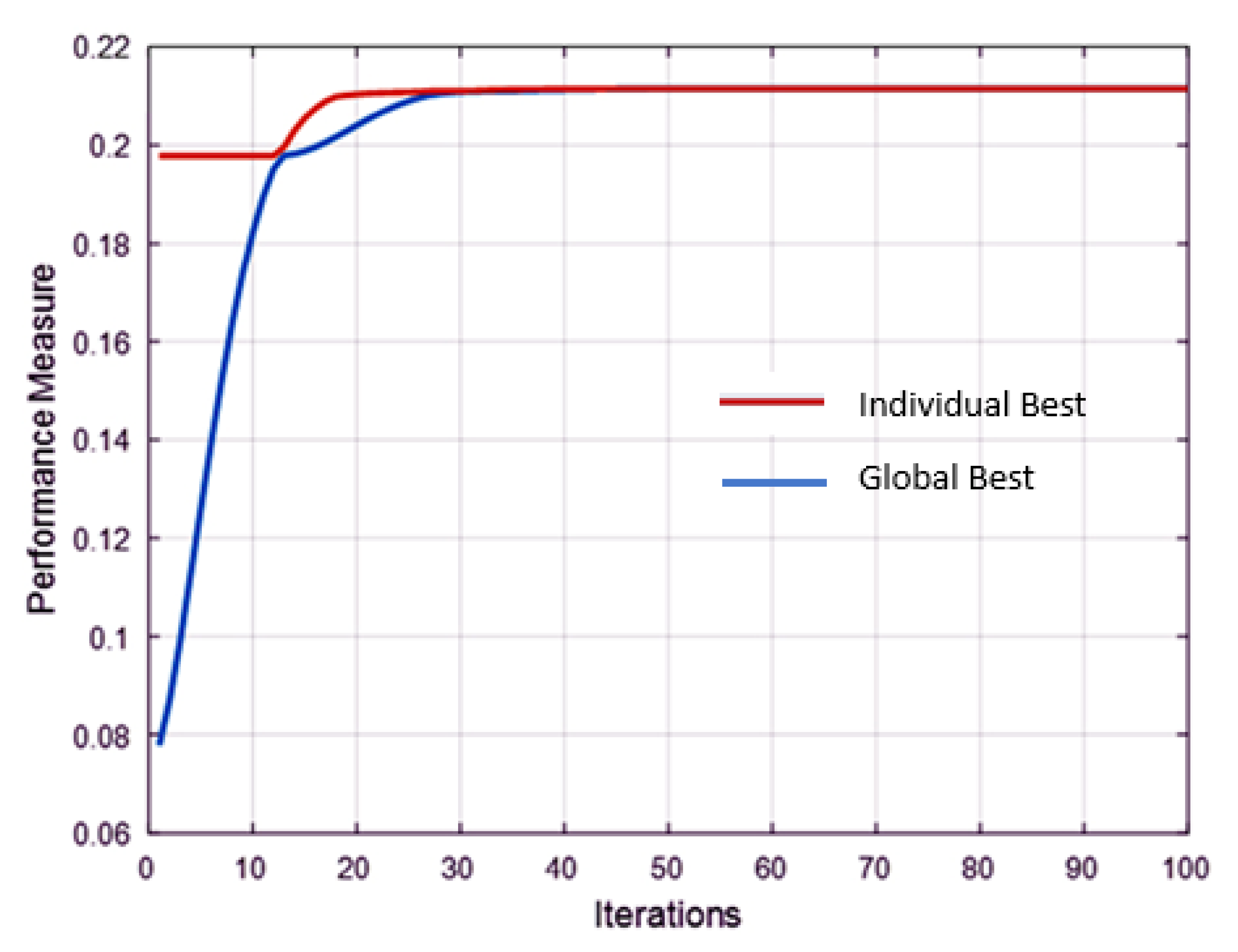
3.2. Implementation of Particle Swarm Optimization (PSO)

The PM model was solved using PSO [47,48], where initially one objective function is formed in Matlab using mathworks. There are two types of solutions in the PSO: global best and individual best. Once the iteration starts, the best value of PM is obtained. As the iteration starts, different solutions are obtained and finally the best solution is obtained, which is the global best. The position at which the global best is predicted is the setting of the input parameter. The PM should be maximum; therefore, the larger it is, the better the type of quality attribute is considered in the present work. The objective function of PM is developed, and the lower and upper limits of each parameter are defined. The lower and upper bounds of each input parameter are provided in Equations (5)–(7).
75 S p e e d 150
0.1 D o C 0.25
0.05 F e e d 0.2
The average processing time for solving the above empirical model by PSO is 21 s (on an Intel i5 processor with 8 GB RAM), which is the average of seven trials. The coefficients (acceleration, C1, and C2) are equal to 1, while the minimum and maximum values of inertia are 0.1 and 0.4, respectively. The swarm size for solving the current problem is equal to 50, and the number of iterations is equal to 100. The best solution predicted by PSO is represented in Figure 6, where it has been identified that the best solution of PM is 0.2114, corresponding to CS: 118 m/min, DoC: 0.22, and F: 0.2. This is the optimum setting suggested by PSO. The experimental setting does not exist in the experimental plan. Therefore, no experiment was conducted in this setting (except during validation experimentations). The nearby trade-off setting is CS: 125 m/min; DoC: 0.2; and F: 0.2 and the corresponding responses are Ra W: 0.752 μm; Ra C: 1.877 μm; and MRR: 5000 mm3/min. Thus, an improvement in the response values has been observed at the optimized setting suggested by PSO. After 27 iterations, the maximum PM value is achieved, and after that, it remains constant up to 100 iterations. The population size considered here varies from 20 to 200, keeping the number of iterations at 100. Every time, similar results were obtained, but the time consumption increased. Therefore, the population was kept at 40 with 100 iterations (complete details are provided in Appendix C). The code is developed using MATLAB. It is a custom-developed script utilizing built-in MATLAB functions and user-defined functions.
The validation experiments are performed at the parameter setting suggested by PSO and are compared with the trial run identified by the MOORA method alone, i.e., test number 64 (Table 3). From the validation table, it is clear that the optimized setting suggested by MOORA is different from the ML-MOORA-PSO and therefore the response variables also differ. The Ra values for wiper (0.59 µm) and conventional (1.30 µm) cases are better in ML-MOORA-PSO than the MOORA (0.735 µm and 1.476 µm) method. However, the MRR is better in MOORA (7499.99 mm3/min) as compared to ML-MOORA-PSO (4996.96 mm3/min). One response is better at the cost of the other; thus, Ra is better at the cost of MRR. Therefore, the proposed approach of ML-MOORA-PSO is successfully applied for the optimization of machining parameters while processing AISI 4340 steel using wiper and conventional tool inserts. The surface quality while machining using the wiper tool insert is 50% greater than the AISI 4340 steel machined by conventional tool inserts.

4. Computational Experience

The XGBoost model of ML was employed for the optimization of machining parameters. A total of 64 experiments were conducted and out of those, 70% were used for training purposes and the rest were for testing purposes. The R 4.3.0 software, along with the library (of XGBoost, caret, rpart, rattle, corrplot, and others for data processing and visualization), were used for the processing of data. The hardware used for the ML approach is an Intel Core i5 processor (8th generation) with 8 GB RAM. Here, XGBoost is used for gradient boosting, caret for parameter tuning, and cross-validation and ggplot2 is used for visualizations. The processing time for each fold is ~15 s. The other parameters (like hyperparameters, cross-validation, and performance validation) for XGBoost are given below.
Hyperparameters: the booster type—‘gbtree’; evaluation metric—RMSE; gamma—0; minimum child weight—1; column sampling ratio (colsample bytree)—1; subsample ratio—1; maximum depth—6; learning rate (eta)—0.3. The early stopping round was set at 20 to stop training (if validation performance did not improve).
Cross-validation: The five-fold cross-validation scheme was employed using a caret package (R Programming, R 4.4.1). The turning grid has the following characteristics:
Minimum child weight—1, 2, 3; column sampling ratio— 0.9, 1; subsample—0.9, 1; maximum depth—2, 4, 6, 8; learning rate (eta)—0.05; 0.1, 0.3; number of round (nrounds)—200 to 1800 (step size of 200).
Performance matrix for MRR is R2—0.98; mean absolute percentage error is (MAPE)—±3%; for Ra, it is R2—0.99; MAPE—±2.5%.

5. Conclusions

The experimental results of previously machined AISI 4340 alloy steel using both wiper geometry and conventional tool inserts provided a robust dataset for training, testing, and validating the machine learning (ML) approach. Based on the comprehensive analysis conducted, the following conclusions can be drawn:
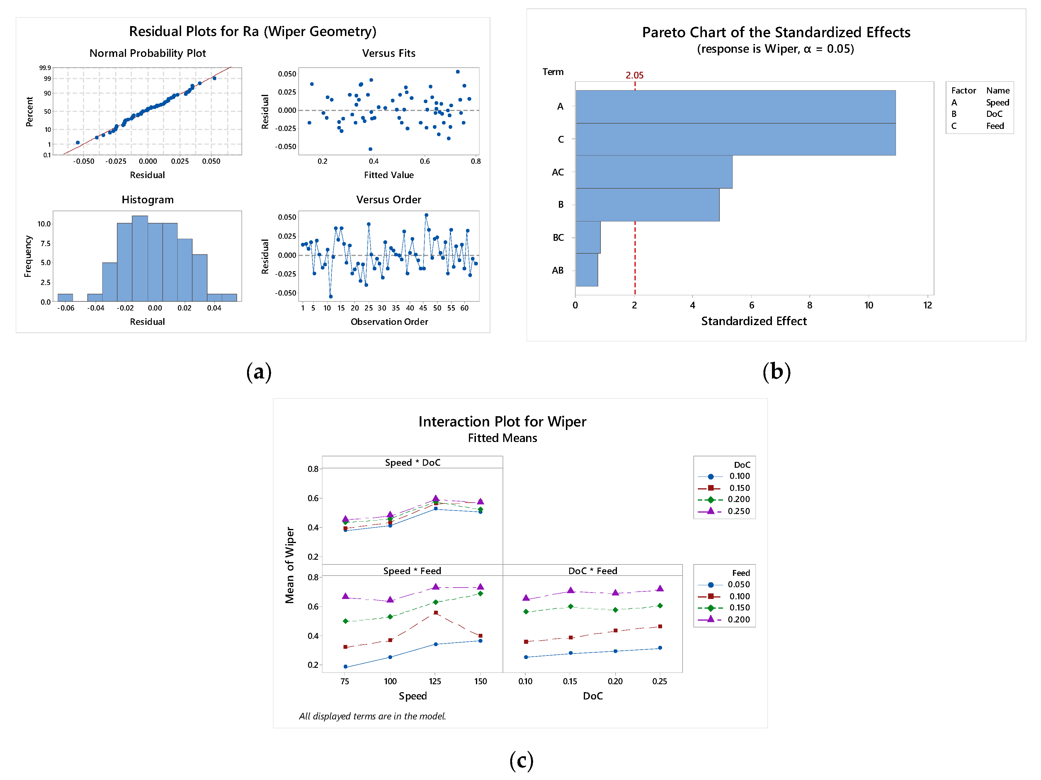
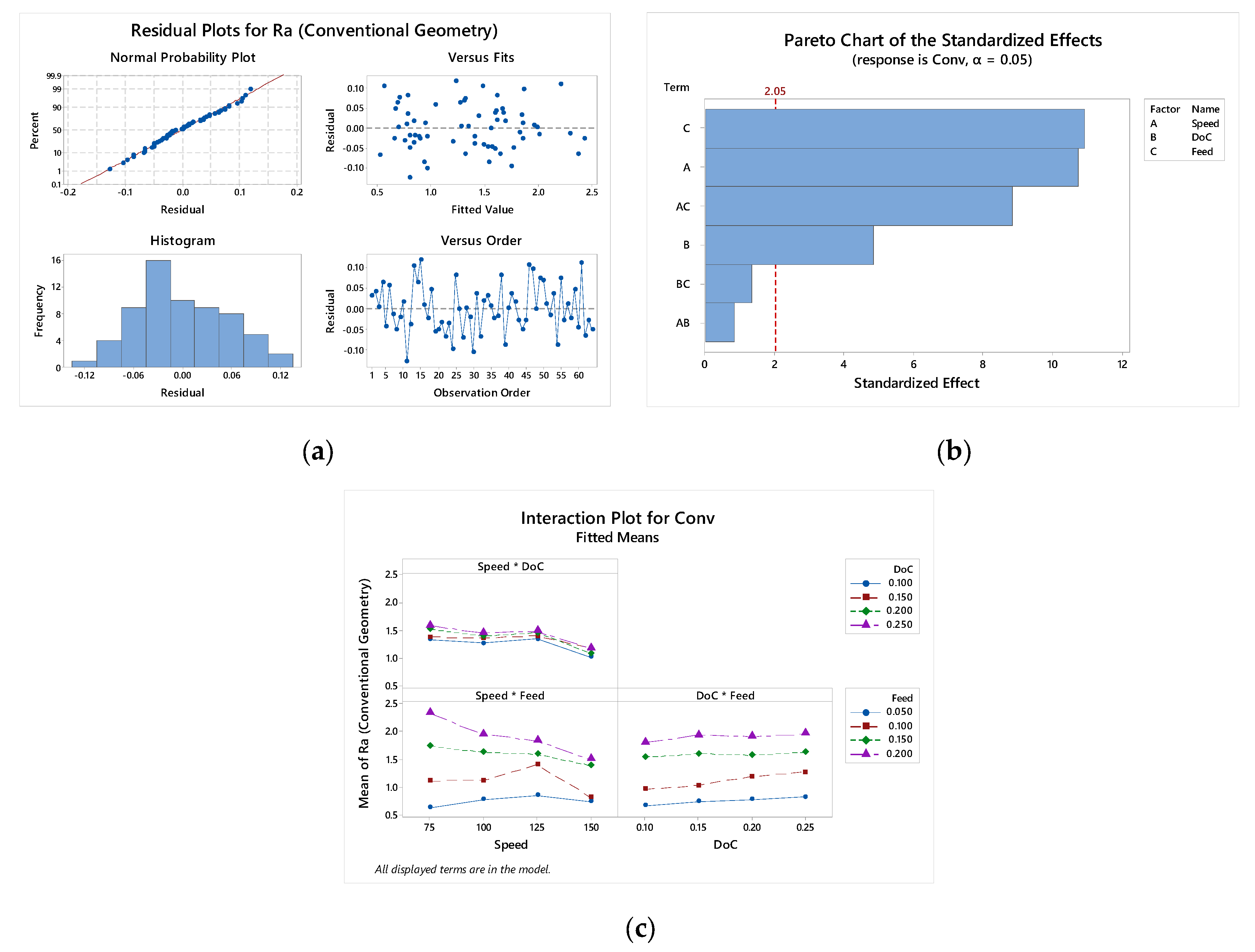
  • The findings revealed that the variation in Ra with respect to depth of cut (DoC) was relatively small, increasing from 0.48 µm to 0.52 µm as DoC increased from 0.1 mm to 0.25 mm. This slight increase is attributed to the larger engagement of the tool in the workpiece, which results in the removal of larger craters, thereby marginally increasing surface roughness. Additionally, Ra increased significantly from 0.29 µm to 0.7 µm as the feed rate (f) increased from 0.05 mm/rev to 0.2 mm/rev due to the increased material removal per revolution, leading to larger craters on the machined surface. Conversely, a higher cutting speed (CS) led to a reduction in Ra, likely due to the minimization of built-up edge formation, which enhances surface quality.
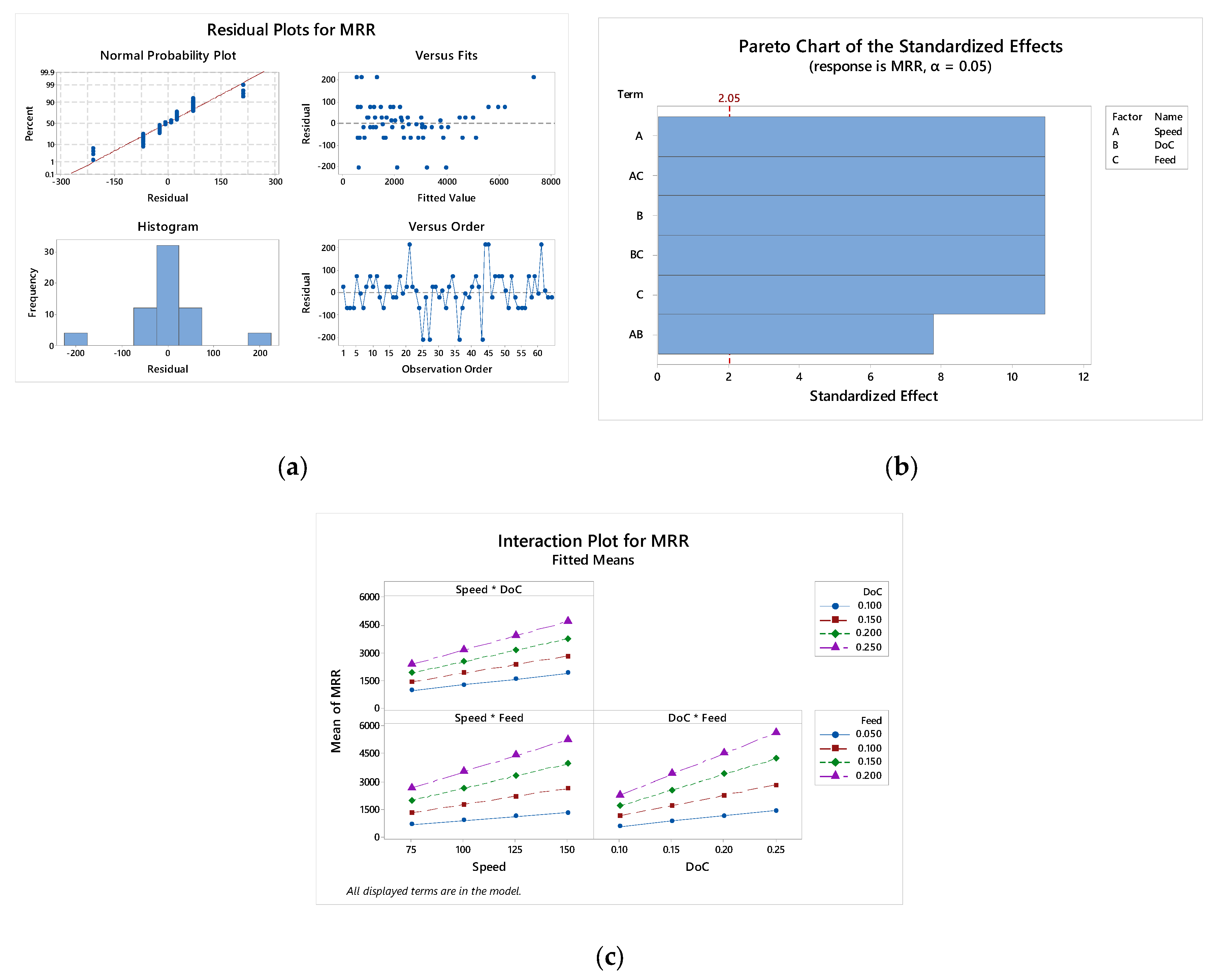
  • The study also highlighted the effect of machining parameters on MRR. It was observed that MRR increased from 1600 mm3/min to 3400 mm3/min with increasing CS, as a higher cutting speed enables more material removal in a given time. Similarly, MRR increased with increasing DoC and f, which is attributed to the greater volume of material engaged in cutting.
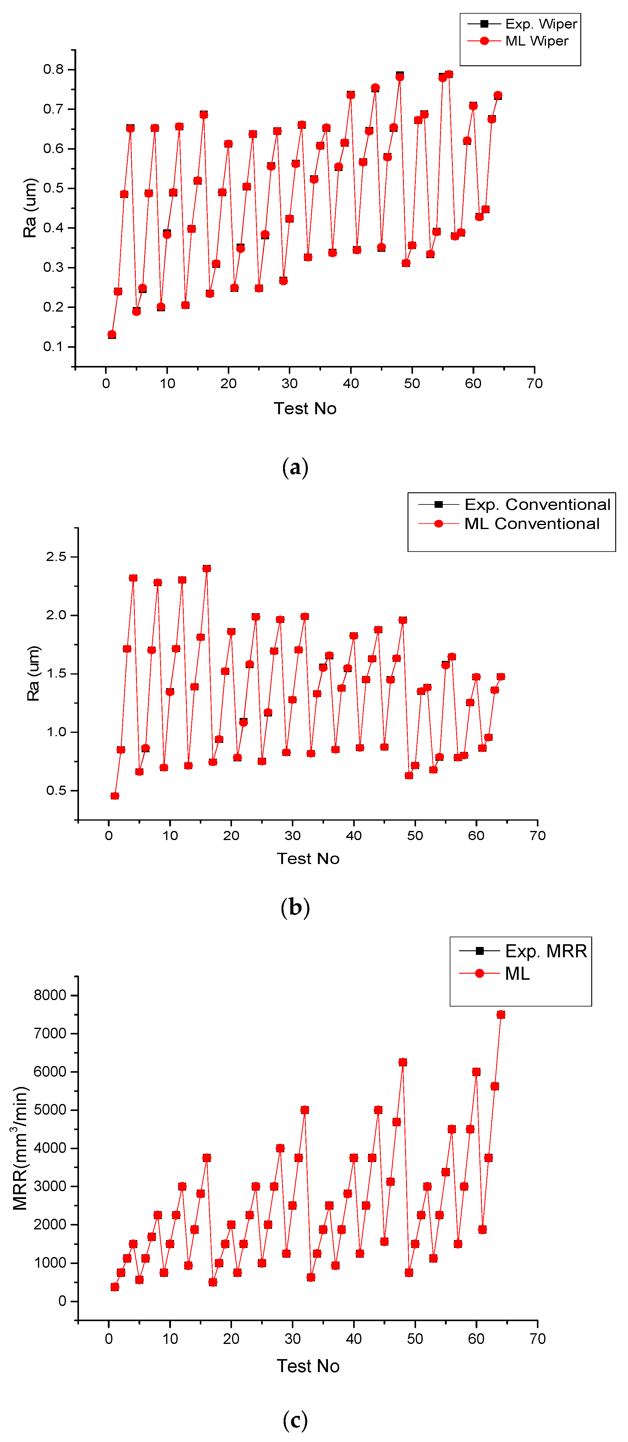
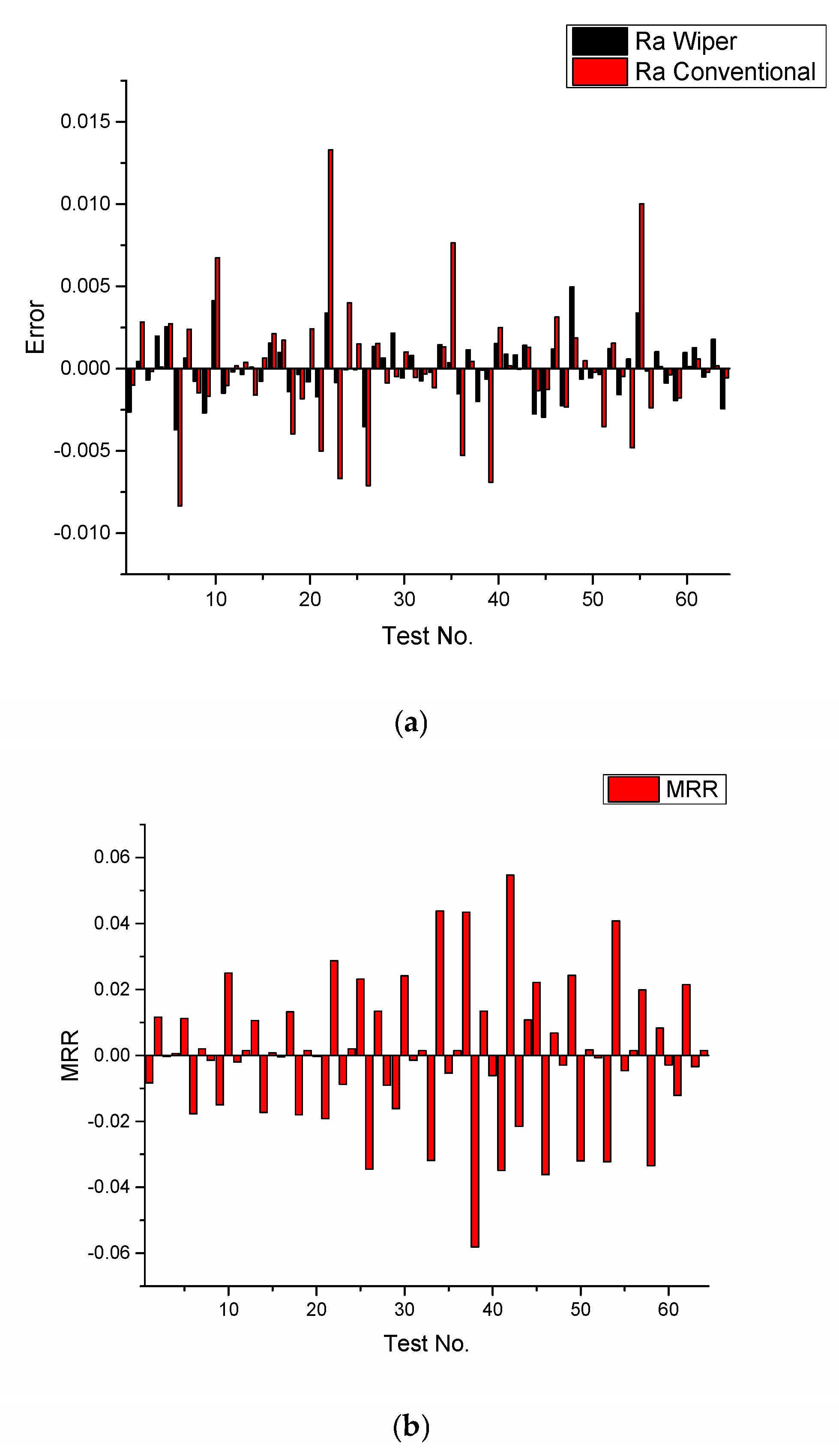
  • Statistical analysis confirmed the reliability of the predictive models. The coefficient of determination (R2) values for Ra and MRR exceeded 99%, indicating a high degree of accuracy in ML-based predictions. The analysis of errors revealed minimal deviations between experimental and predicted values, affirming the robustness of the ML model.
  • A comparative assessment of wiper and conventional tool inserts demonstrated that wiper geometry provides superior surface quality due to its secondary cutting edge, which eliminates microscopic ridges. The mean square error (MSE) for Ra was found to be lower for wiper inserts compared to conventional inserts, further validating the enhanced performance of wiper geometry in achieving better machining responses.
The combination of machine learning, MOORA, and particle swarm optimization (PSO) in this study not only optimized machining parameters but also highlighted the effectiveness of this hybrid approach in improving machining outcomes. This approach holds substantial potential for further exploration in areas such as dimensional accuracy, chip morphology, cutting forces, residual stresses, and temperature control during machining operations. Moreover, the versatility of this method suggests that its application could be extended to other manufacturing processes, including milling, drilling, and non-conventional machining techniques, broadening its industrial applicability.
The implications for real-world manufacturers are enhanced productivity and quality, cost saving, and sustainability. The use of wiper inserts improves the surface roughness and MRR, which enhances productivity and quality. The improved surface finish eliminates the secondary finishing operations, which leads to cost savings. A challenge associated with implementation is the integration into existing software, which requires software upgrades. Another challenge is associated with data collection for ML prediction. Manufacturers may face challenges in collecting consistent machining data due to variations in material properties, tooling conditions, and machine dynamics.

Author Contributions

A.T.A., N.S. and K.F.A.: investigation, conceptualization, methodology, data curation, validation, visualization. A.E., R.C.S. and M.A.A.: software, investigation, writing—original draft, writing, conceptualization, supervision, project administration, writing—review and editing, K.F.A.: funding acquisition. All authors have read and agreed to the published version of the manuscript.

Funding

King Saud University—Project number (RSPD2025R827).

Data Availability Statement

All data generated or analyzed during this study are included in this published article.

Acknowledgments

The authors thank King Saud University for funding this work through the Researchers Supporting Project number (RSPD2025R827), King Saud University, Riyadh, Saudi Arabia.

Conflicts of Interest

The authors declare that they have no known conflicts of interest.

Appendix A

Table A1. Experimental array and the corresponding results.
TestSpeedDepth of CutFeedSurface Roughness, Ra, (μm)MRRTestSpeedDepth of CutFeedSurface Roughness, Ra, (μm)MRR
No.(m/min)(mm)(mm/rev)WiperConv.(mm3/min)No.(m/min)(mm)(mm/rev)WiperConv.(mm3/min)
1750.10.050.1290.454375331250.10.050.3260.817625
2750.10.10.240.851750341250.10.10.5241.3311250
3750.10.150.4851.7131125351250.10.150.6081.5581875
4750.10.20.6532.321500361250.10.20.6521.6542500
5750.150.050.1910.663562.5371250.150.050.3380.852937.5
6750.150.10.2450.8581125381250.150.10.5531.3771875
7750.150.150.4881.7041687.5391250.150.150.6151.5442812.5
8750.150.20.6522.282250401250.150.20.7371.8273750
9750.20.050.1990.696750411250.20.050.3450.8671250
10750.20.10.3871.3491500421250.20.10.5671.4512500
11750.20.150.4891.7142250431250.20.150.6461.6293750
12750.20.20.6562.3033000441250.20.20.7521.8775000
13750.250.050.2050.715937.5451250.250.050.3490.8731562.5
14750.250.10.3981.3881875461250.250.10.581.4513125
15750.250.150.5191.8142812.5471250.250.150.6521.6314687.5
16750.250.20.6872.4023750481250.250.20.7861.966250
171000.10.050.2350.746500491500.10.050.3110.629750
181000.10.10.3090.9381000501500.10.10.3560.7161500
191000.10.150.491.5211500511500.10.150.6721.3482250
201000.10.20.6121.8622000521500.10.20.6881.3843000
211000.150.050.2480.78750531500.150.050.3330.6781125
221000.150.10.3511.0941500541500.150.10.3910.7852250
231000.150.150.5041.5772250551500.150.150.7821.5813375
241000.150.20.6371.9893000561500.150.20.7881.6454500
251000.20.050.2480.7521000571500.20.050.380.7831500
261000.20.10.3811.1652000581500.20.10.3880.8023000
271000.20.150.5571.6953000591500.20.150.6191.2534500
281000.20.20.6451.9644000601500.20.20.7091.4746000
291000.250.050.2680.8271250611500.250.050.4290.8641875
301000.250.10.4231.2792500621500.250.10.4470.9563750
311000.250.150.5631.7043750631500.250.150.6761.3615625
321000.250.20.661.995000641500.250.20.7331.4757500
Table A2. Analysis of variance.
Ra (Wiper Geometry)
SourceDFSSMSF-Valuep-Value
Model361.968700.05468651.790.000
 Linear91.872900.208100197.080.000
  Speed30.258680.08622881.660.000
  DoC30.037580.01252711.860.000
  Feed31.576630.525545497.700.000
 2-Way Interactions270.095800.0035483.360.001
  Speed × DoC90.009630.0010701.010.454
  Speed × Feed90.075880.0084327.980.000
  DoC × Feed90.010290.0011441.080.406
Error270.028510.001056
Total631.99721S: 0.0324952; R2: 98.57%; Adj R2: 96.67%; R2 Pred.: 91.98%
Ra (Conventional Geometry)
Model3615.29340.4248255.630.000
 Linear913.81811.53535201.060.000
  Speed31.16790.3893050.980.000
  DoC30.26610.0887111.620.000
  Feed312.38414.12804540.580.000
 2-Way Interactions271.47530.054647.160.000
  Speed × DoC90.07460.008291.090.404
  Speed × Feed91.29550.1439518.850.000
  DoC × Feed90.10510.011681.530.188
Error270.20620.00764
Total6315.4996S: 0.0873863; R2: 98.67%; Adj R2: 96.90%; R2 Pred.: 92.53%
MRR
Model3615,61,32,81243,37,023239.820.000
 Linear914,09,96,09415,66,62,33866.280.000
  Speed32,39,25,78179,75,260441.000.000
  DoC33,95,50,7811,31,83,594729.000.000
  Feed37,75,19,5312,58,39,8441428.840.000
 2-Way Interactions271,51,36,7195,60,61931.000.000
  Speed × DoC924,41,4062,71,26715.000.000
  Speed × Feed947,85,1565,31,68429.400.000
  DoC × Feed979,10,1568,78,90648.600.000
Error274,88,28118,084
Total6315,66,21,094S: 134.479; R2: 99.69%; Adj R2: 99.27%; R2 Pred.: 98.25%
Figure A1. Analysis of Ra (wiper geometry).
Processes 13 01156 g0a1
Figure A2. Analysis of Ra (conventional geometry).
Processes 13 01156 g0a2
Figure A3. Analysis of MRR.
Processes 13 01156 g0a3

Appendix B

Hyperparameter Selection Justification:
  • Booster Type (‘gbtree’): The ‘gbtree’ booster was selected because it is well-suited for handling structured data with complex interactions among features. Given that machining parameters have non-linear relationships, tree-based models generally perform better than linear models (‘gblinear’).
  • Evaluation Metric (RMSE): Root Mean Squared Error (RMSE) was chosen as the primary evaluation metric because it effectively measures prediction accuracy while penalizing large errors, which is crucial in machining optimization, where precise control over parameters is needed.
  • Gamma (0): A gamma value of 0 was chosen to allow all splits initially and then fine-tune based on performance. Higher values of gamma would restrict tree splitting, which was not required for the given dataset size and complexity.
  • Minimum Child Weight (1): A lower child weight ensures that even smaller subgroups in data are considered while splitting nodes. This helps in capturing variations in machining parameters without overfitting.
  • Column Sampling Ratio (1): A full column sample (colsample_bytree = 1) was initially selected to allow the model to consider all features and ensure no relevant information was ignored. However, fine-tuning was conducted using values of 0.9 and 1.
  • Subsample Ratio (1): A full subsample was initially chosen to avoid introducing randomness. Further optimization was performed by testing subsample values of 0.9 and 1 to observe its effect on model stability.
  • Maximum Depth (6): This value was selected to balance model complexity and performance. A deeper tree might overfit, while a shallower tree might underfit. A tuning grid was tested for depths of 2, 4, 6, and 8 to optimize this tradeoff.
  • Learning Rate (Eta = 0.3): A learning rate of 0.3 was selected based on empirical studies, which suggest that for boosting methods, an initial eta in the range of 0.1–0.3 often provides a good balance between convergence speed and performance. Lower values (0.05, 0.1) were also tested for further refinement.
  • Early Stopping (20 rounds): The stopping criterion of 20 rounds was used to prevent overfitting. If the validation score did not improve over 20 consecutive rounds, training was stopped to save computational resources.
Cross-Validation Justification:
  • Five-Fold Cross-Validation: A 5-fold scheme was used as a standard practice in machine learning to balance computational efficiency and model reliability. Increasing folds (e.g., 10-fold) would increase computation time significantly, while fewer folds (e.g., 3-fold) might not generalize well.
  • Tuning Grid Selection: The parameter grid was selected based on prior literature and empirical testing. The chosen ranges ensured a comprehensive search space without excessive computational overhead.
Performance Metrics Justification:
  • R2 and MAPE: R2 was chosen as a performance measure to evaluate how well the model explains variance in the machining performance outputs (MRR, Ra). Mean absolute percentage error (MAPE) was used to assess the relative error percentage, ensuring practical significance in real-world applications. The obtained values (R2 > 0.98 and MAPE < 3%) indicate a well-optimized model with high predictive accuracy.

Appendix C

  • Population Size (Swarm Size): 40; Maximum Iterations: 100;
  • Constriction Coefficients: kappa = 1;
  • phi1 = 2.05;
  • phi2 = 2.05;
  • chi = 2 ∗ kappa/abs (2-phi-sqrt (phi2 − 4 ∗ phi))
  • Inertia Coefficient: w = chi
  • Damping Ratio of Inertia Weight: wdamp = 1
  • Personal and Social Acceleration Coefficients:
  • c1 = chi ∗ phi1
  • c2 = chi ∗ phi2
  • Randomization Factors:
  • r1 = 0.9706
  • r2 = 0.0318
  • Velocity Constraints:
  • MaxVelocity = 0.2 ∗ (VarMax − VarMin)
  • MinVelocity = −MaxVelocity

References

  1. He, K.; Gao, M.; Zhao, Z. Soft Computing Techniques for Surface Roughness Prediction in Hard Turning: A Literature Review. IEEE Access 2019, 7, 89556–89569. [Google Scholar] [CrossRef]
  2. Grzesik, W. Wear Development on Wiper Al2O3–TiC Mixed Ceramic Tools in Hard Machining of High Strength Steel. Wear 2009, 266, 1021–1028. [Google Scholar] [CrossRef]
  3. D’Addona, D.M.; Raykar, S.J. Thermal Modeling of Tool Temperature Distribution during High Pressure Coolant Assisted Turning of Inconel 718. Materials 2019, 12, 408. [Google Scholar] [CrossRef] [PubMed]
  4. Abbas, A.T.; Gupta, M.K.; Soliman, M.S.; Mia, M.; Hegab, H.; Luqman, M.; Pimenov, D.Y. Sustainability Assessment Associated with Surface Roughness and Power Consumption Characteristics in Nanofluid MQL-Assisted Turning of AISI 1045 Steel. Int. J. Adv. Manuf. Technol. 2019, 105, 1311–1327. [Google Scholar] [CrossRef]
  5. Díaz-Álvarez, J.; Díaz-Álvarez, A.; Miguélez, H.; Cantero, J.L. Finishing Turning of Ni Superalloy Haynes 282. Metals 2018, 8, 843. [Google Scholar] [CrossRef]
  6. Abu Qudeiri, J.E.; Saleh, A.; Ziout, A.; Mourad, A.H.I.; Abidi, M.H.; Elkaseer, A. Advanced Electric Discharge Machining of Stainless Steels: Assessment of the State of the Art, Gaps and Future Prospect. Materials 2019, 12, 907. [Google Scholar] [CrossRef]
  7. Saleh, B.; Fathi, R.; Tian, Y.; Radhika, N.; Jiang, J.; Ma, A. Fundamentals and Advances of Wire Arc Additive Manufacturing: Materials, Process Parameters, Potential Applications, and Future Trends. Arch. Civ. Mech. Eng. 2023, 23, 96. [Google Scholar] [CrossRef]
  8. Gaitonde, V.N.; Karnik, S.R.; Figueira, L.; Davim, J.P. Machinability Investigations in Hard Turning of AISI D2 Cold Work Tool Steel with Conventional and Wiper Ceramic Inserts. Int. J. Refract. Met. Hard Mater. 2009, 27, 754–763. [Google Scholar] [CrossRef]
  9. Kumar, P.; Chauhan, S.R.; Pruncu, C.I.; Gupta, M.K.; Pimenov, D.Y.; Mia, M.; Gill, H.S. Influence of Different Grades of CBN Inserts on Cutting Force and Surface Roughness of AISI H13 Die Tool Steel during Hard Turning Operation. Materials 2019, 12, 177. [Google Scholar] [CrossRef]
  10. Zhang, S.J.; To, S.; Wang, S.J.; Zhu, Z.W. A Review of Surface Roughness Generation in Ultra-Precision Machining. Int. J. Mach. Tools Manuf. 2015, 91, 76–95. [Google Scholar] [CrossRef]
  11. Podgornik, B.; Sedlaček, M.; Žužek, B.; Guštin, A. Properties of Tool Steels and Their Importance When Used in a Coated System. Coatings 2020, 10, 265. [Google Scholar] [CrossRef]
  12. Kishawy, H.A.; Hegab, H.; Umer, U.; Mohany, A. Application of Acoustic Emissions in Machining Processes: Analysis and Critical Review. Int. J. Adv. Manuf. Technol. 2018, 98, 1391–1407. [Google Scholar] [CrossRef]
  13. Bilal, M.M.; Yaqoob, K.; Zahid, M.H.; Tanveer, W.H.; Wadood, A.; Ahmed, B. Effect of Austempering Conditions on the Microstructure and Mechanical Properties of AISI 4340 and AISI 4140 Steels. J. Mater. Res. Technol. 2019, 8, 5194–5200. [Google Scholar] [CrossRef]
  14. Astakhov, V.P. Machining of Hard Materials–Definitions and Industrial Applications. In Machining of Hard Materials; Springer: London, UK, 2011; pp. 1–32. [Google Scholar]
  15. Bhattacharyya, B.; Doloi, B. Modern Machining Technology: Advanced, Hybrid, Micro Machining and Super Finishing Technology; Academic Press: New York, NY, USA, 2019. [Google Scholar]
  16. Patwari, M.A.U.; Mahmood, M.N.; Noor, S.; Shovon, M.Z.H. Investigation of Machinability Responses during Magnetic Field Assisted Turning Process of Preheated Mild Steel. Procedia Eng. 2013, 56, 713–718. [Google Scholar] [CrossRef]
  17. Flórez García, L.C.; González Rojas, H.A.; Sánchez Egea, A.J. Estimation of Specific Cutting Energy in an S235 Alloy for Multi-Directional Ultrasonic Vibration-Assisted Machining Using the Finite Element Method. Materials 2020, 13, 567. [Google Scholar] [CrossRef]
  18. Xu, Y.; Gong, Y.; Zhang, W.; Wen, X.; Xin, B.; Zhang, H. Effect of Grinding Conditions on the Friction and Wear Performance of Ni-Based Singlecrystal Superalloy. Arch. Civ. Mech. Eng. 2022, 22, 102. [Google Scholar] [CrossRef]
  19. Yap, T.C. Roles of Cryogenic Cooling in Turning of Superalloys, Ferrous Metals, and Viscoelastic Polymers. Technologies 2019, 7, 63. [Google Scholar] [CrossRef]
  20. Joch, R.; Pilc, J.; Daniš, I.; Drbúl, M.; Krajčoviech, S. Analysis of Surface Roughness in Turning Process Using Rotating Tool with Chip Breaker for Specific Shapes of Automotive Transmission Shafts. Transp. Res. Procedia 2019, 40, 295–301. [Google Scholar] [CrossRef]
  21. Subbaiah, K.V.; Raju, C.; Pawade, R.S.; Suresh, C. Machinability Investigation with Wiper Ceramic Insert and Optimization during the Hard Turning of AISI 4340 Steel. Mater. Today Proc. 2019, 18, 445–454. [Google Scholar] [CrossRef]
  22. Chinchanikar, S.; Kore, S.S.; Hujare, P. A Review on Nanofluids in Minimum Quantity Lubrication Machining. J. Manuf. Process. 2021, 68, 56–70. [Google Scholar] [CrossRef]
  23. Weinert, K.; Inasaki, I.; Sutherland, J.W.; Wakabayashi, T. Dry Machining and Minimum Quantity Lubrication. CIRP Ann. 2004, 53, 511–537. [Google Scholar] [CrossRef]
  24. De Maddis, M.; Lunetto, V.; Razza, V.; Russo Spena, P. Infrared Thermography for Investigation of Surface Quality in Dry Finish Turning of Ti6Al4V. Metals 2022, 12, 154. [Google Scholar] [CrossRef]
  25. Sreejith, P.S.; Ngoi, B.K.A. Dry Machining: Machining of the Future. J. Mater. Process. Technol. 2000, 101, 287–291. [Google Scholar] [CrossRef]
  26. Elsheikh, A.H.; Abd Elaziz, M.; Das, S.R.; Muthuramalingam, T.; Lu, S. A New Optimized Predictive Model Based on Political Optimizer for Eco-Friendly MQL-Turning of AISI 4340 Alloy with Nano-Lubricants. J. Manuf. Process. 2021, 67, 562–578. [Google Scholar] [CrossRef]
  27. Padhan, S.; Das, S.R.; Das, A.; Alsoufi, M.S.; Ibrahim, A.M.M.; Elsheikh, A. Machinability Investigation of Nitronic 60 Steel Turning Using SiAlON Ceramic Tools under Different Cooling/Lubrication Conditions. Materials 2022, 15, 2368. [Google Scholar] [CrossRef]
  28. Çamlı, K.Y.; Demirsöz, R.; Boy, M.; Korkmaz, M.E.; Yaşar, N.; Giasin, K.; Pimenov, D.Y. Performance of MQL and Nano-MQL Lubrication in Machining ER7 Steel for Train Wheel Applications. Lubricants 2022, 10, 48. [Google Scholar] [CrossRef]
  29. Etri, H.E.L.; Singla, A.K.; Özdemir, M.T.; Korkmaz, M.E.; Demirsöz, R.; Gupta, M.K.; Krolczyk, J.B.; Ross, N.S. Wear Performance of Ti-6Al-4 V Titanium Alloy through Nano-Doped Lubricants. Arch. Civ. Mech. Eng. 2023, 23, 147. [Google Scholar] [CrossRef]
  30. Chen, T.; Guestrin, C. XGBoost: A scalable tree boosting system. In Proceedings of the 22nd ACM SIGKDD International Conference on Knowledge Discovery and Data Mining, San Francisco, CA, USA, 13–17 August 2016. [Google Scholar]
  31. Charalampous, P. Prediction of Cutting Forces in Milling Using Machine Learning Algorithms and Finite Element Analysis. J. Mater. Eng. Perform. 2021, 30, 2002–2013. [Google Scholar] [CrossRef]
  32. Gao, S.; Wang, H.; Huang, H.; Dong, Z.; Kang, R. Predictive models for the surface roughness and subsurface damage depth of semiconductor materials in precision grinding. Int. J. Extrem. Manuf. 2025, 7, 035103. [Google Scholar] [CrossRef]
  33. Korkmaz, M.E.; Gupta, M.K.; Kuntoğlu, M.; Patange, A.D.; Ross, N.S.; Yılmaz, H.; Chauhan, S.; Vashishtha, G. Prediction and classification of tool wear and its state in sustainable machining of Bohler steel with different machine learning models. Measurement 2023, 223, 113825. [Google Scholar] [CrossRef]
  34. Ross, N.S.; Mashinini, P.M.; Shibi, C.S.; Gupta, M.K.; Korkmaz, M.E.; Krolczyk, G.M.; Sharma, V.S. A new intelligent approach of surface roughness measurement in sustainable machining of AM-316L stainless steel with deep learning models. Measurement 2024, 230, 114515. [Google Scholar] [CrossRef]
  35. Zhang, P.R.; Liu, Z.Q.; Guo, Y.B. Machinability for Dry Turning of Laser Cladded Parts with Conventional vs. Wiper Insert. J. Manuf. Process. 2017, 28, 494–499. [Google Scholar] [CrossRef]
  36. Jiang, L.; Wang, D. Finite-Element-Analysis of the Effect of Different Wiper Tool Edge Geometries during the Hard Turning of AISI 4340 Steel. Simul. Model. Pract. Theory 2019, 94, 250–263. [Google Scholar] [CrossRef]
  37. Kuntoğlu, M.; Sağlam, H. Investigation of signal behaviors for sensor fusion with tool condition monitoring system in turning. Measurement 2021, 173, 108582. [Google Scholar] [CrossRef]
  38. Asiltürk, İ.; Kuntoğlu, M.; Binali, R.; Akkuş, H.; Salur, E. A comprehensive analysis of surface roughness, vibration, and acoustic emissions based on machine learning during hard turning of AISI 4140 steel. Metals 2023, 13, 437. [Google Scholar] [CrossRef]
  39. Goyal, K.K.; Sharma, N.; Gupta, R.D.; Gupta, S.; Rani, D.; Kumar, D.; Sharma, V.S. Measurement of Performance Characteristics of WEDM While Processing AZ31 Mg-Alloy Using Levy Flight MOGWO for Orthopedic Application. Int. J. Adv. Manuf. Technol. 2022, 119, 7175–7197. [Google Scholar] [CrossRef]
  40. Chi, Y.; Dong, Z.; Cui, M.; Shan, C.; Xiong, Y.; Zhang, D.; Luo, M. Comparative study on machinability and surface integrity of γ-TiAl alloy in laser assisted milling. J. Mater. Res. Technol. 2024, 33, 3743–3755. [Google Scholar] [CrossRef]
  41. Abbas, A.T.; El Rayes, M.M.; Luqman, M.; Naeim, N.; Hegab, H.; Elkaseer, A. On the Assessment of Surface Quality and Productivity Aspects in Precision Hard Turning of AISI 4340 Steel Alloy: Relative Performance of Wiper vs. Conventional Inserts. Materials 2020, 13, 2036. [Google Scholar] [CrossRef]
  42. Abbas, A.T.; Anwar, S.; Hegab, H.; Benyahia, F.; Ali, H.; Elkaseer, A. Comparative Evaluation of Surface Quality, Tool Wear, and Specific Cutting Energy for Wiper and Conventional Carbide Inserts in Hard Turning of AISI 4340 Alloy Steel. Materials 2020, 13, 5233. [Google Scholar] [CrossRef]
  43. Brauers, W.K.; Zavadskas, E.K. The MOORA Method and Its Application to Privatization in a Transition Economy. Control Cybern. 2006, 35, 445–469. [Google Scholar]
  44. Murat, S.; Gupta, M.K.; Tomaz, I.; Pimenov, D.Y.; Kuntoğlu, M.; Khanna, N.; Yıldırım, Ç.V.; Krolczyk, G.M. A state-of-the-art review on tool wear and surface integrity characteristics in machining of superalloys. CIRP J. Manuf. Sci. Technol. 2021, 35, 624–658. [Google Scholar]
  45. Yu, P.D.; da Silva, L.R.R.; Machado, A.R.; França, P.H.P.; Pintaude, G.; Unune, D.R.; Kuntoğlu, M.; Krolczyk, G.M. A comprehensive review of machinability of difficult-to-machine alloys with advanced lubricating and cooling techniques. Tribol. Int. 2024, 196, 109677. [Google Scholar]
  46. Machado, A.R.; da Silva, L.R.R.; Pimenov, D.Y.; de Souza, F.C.R.; Kuntoğlu, M.; de Paiva, R.L. Comprehensive review of advanced methods for improving the parameters of machining steels. J. Manuf. Process. 2024, 125, 111–142. [Google Scholar] [CrossRef]
  47. Kennedy, J.; Eberhart, R. Particle swarm optimization. In Proceedings of the ICNN’95-International Conference on Neural Networks, Perth, WA, Australia, 27 November 1995; Volume 4, pp. 1942–1948. [Google Scholar]
  48. Wang, D.; Tan, D.; Liu, L. Particle swarm optimization algorithm: An overview. Soft Comput. 2018, 22, 387–408. [Google Scholar] [CrossRef]
Figure 1. Process flow adopted in the present research.
Processes 13 01156 g001
Figure 2. Variation in (a) Ra (wiper), (b) Ra (conventional insert), and (c) MRR, with respect to process parameters (coolant flow rate: 12 L/min; temperature: 24 °C).
Processes 13 01156 g002
Figure 3. Experimental and predicted (by ML) values for (a) Ra (Wiper geometry), (b) Ra (Conventional tool), and (c) MRR.
Processes 13 01156 g003
Figure 4. Error values for (a) Ra (wiper geometry), Ra (conventional tool), and (b) MRR.
Processes 13 01156 g004
Figure 5. (a) Numerical Correlation plot of input machining parameters and response variables (b) Correlation plot as per the Colour Code (c) Percentage influence of each parameter on Response (d) Variation of input parameters on response variable (e) Predicted versus Actual plot for responses (f) Mean Square error and R2 for different responses.
Processes 13 01156 g005aProcesses 13 01156 g005b
Figure 6. Variation in performance measure with the iterations using PSO.
Processes 13 01156 g006
Table 1. Input process parameters, units, and levels.
Machining ParametersUnitsLevels of Input Process Parameters
Level 1Level 2Level 3Level 4
CuttingSpeedm/min75100125150
Depth of cut (DoC)mm0.10.150.20.25
Feed rate (f)mm/rev0.050.10.150.2
Table 2. Validation experiments.
PredictedExperimental
MethodSettingPMMRR Ra WRa CMRRRa WRa C
ML-MOORA-PSOCS118DoC0.22F0.20.21144996.960.591.3050000.621.26
MOORACS150DoC0.25F0.20.2077499.9990.7351.47675000.7331.475
Table 3. Normalized value of responses and performance measures.
Test No.Predicted Values MLNormalized DataWeighted Normalized
Decision Matrix
GradeRank
MRRRa (Wiper)Ra (Conv)MRRRa (Wiper)Ra (Conv)MRRRa (Wiper)Ra (Conv)
1375.0080.1320.4550.0160.0310.0400.0050.0100.0130.02964
2749.9880.2400.8480.0320.0570.0740.0110.0190.0250.05457
31125.0000.4861.7130.0480.1160.1500.0160.0380.0500.10437
41499.9990.6512.3200.0640.1560.2040.0210.0510.0670.14019
5562.4890.1880.6600.0240.0450.0580.0080.0150.0190.04263
61125.0180.2490.8660.0480.0590.0760.0160.0200.0250.06154
71687.4980.4871.7020.0720.1170.1490.0240.0380.0490.11233
82250.0010.6532.2810.0960.1560.2000.0320.0520.0660.14916
9750.0150.2020.6980.0320.0480.0610.0110.0160.0200.04762
101499.9750.3831.3420.0640.0920.1180.0210.0300.0390.09042
112250.0020.4901.7150.0960.1170.1510.0320.0390.0500.12029
122999.9990.6562.3030.1290.1570.2020.0420.0520.0670.16112
13937.4890.2050.7150.0400.0490.0630.0130.0160.0210.05060
141875.0170.3981.3900.0800.0950.1220.0270.0310.0400.09838
152812.4990.5201.8130.1210.1240.1590.0400.0410.0530.13323
163750.0000.6852.4000.1610.1640.2110.0530.0540.0700.1776
17499.9870.2340.7440.0210.0560.0650.0070.0180.0220.04761
181000.0180.3100.9420.0430.0740.0830.0140.0250.0270.06650
191499.9990.4901.5230.0640.1170.1340.0210.0390.0440.10436
202000.0000.6131.8600.0860.1470.1630.0280.0480.0540.13126
21750.0190.2500.7850.0320.0600.0690.0110.0200.0230.05359
221499.9710.3481.0810.0640.0830.0950.0210.0270.0310.08045
232250.0090.5051.5840.0960.1210.1390.0320.0400.0460.11831
242999.9980.6371.9850.1290.1520.1740.0420.0500.0570.15015
25999.9770.2480.7510.0430.0590.0660.0140.0200.0220.05556
262000.0350.3851.1720.0860.0920.1030.0280.0300.0340.09341
272999.9870.5561.6930.1290.1330.1490.0420.0440.0490.13521
284000.0090.6441.9650.1710.1540.1720.0570.0510.0570.16410
291250.0160.2660.8270.0540.0640.0730.0180.0210.0240.06352
302499.9760.4241.2780.1070.1010.1120.0350.0330.0370.10635
313750.0010.5621.7050.1610.1340.1500.0530.0440.0490.14718
324999.9990.6611.9900.2140.1580.1750.0710.0520.0580.1815
33625.0320.3260.8180.0270.0780.0720.0090.0260.0240.05855
341249.9560.5231.3300.0540.1250.1170.0180.0410.0390.09739
351875.0050.6081.5500.0800.1450.1360.0270.0480.0450.11930
362499.9990.6541.6590.1070.1560.1460.0350.0520.0480.13522
37937.4570.3370.8520.0400.0810.0750.0130.0270.0250.06551
381875.0580.5551.3770.0800.1330.1210.0270.0440.0400.11034
392812.4870.6161.5510.1210.1470.1360.0400.0490.0450.13324
403750.0060.7351.8250.1610.1760.1600.0530.0580.0530.16411
411250.0350.3440.8670.0540.0820.0760.0180.0270.0250.07049
422499.9450.5661.4510.1070.1350.1270.0350.0450.0420.12228
433750.0210.6451.6280.1610.1540.1430.0530.0510.0470.15114
444999.9890.7551.8780.2140.1810.1650.0710.0600.0540.1853
451562.4780.3520.8740.0670.0840.0770.0220.0280.0250.07546
463125.0360.5791.4480.1340.1380.1270.0440.0460.0420.13225
474687.4930.6541.6330.2010.1560.1430.0660.0520.0470.1659
486250.0030.7811.9580.2680.1870.1720.0880.0620.0570.2072
49749.9760.3120.6290.0320.0750.0550.0110.0250.0180.05358
501500.0320.3570.7160.0640.0850.0630.0210.0280.0210.07048
512249.9980.6721.3520.0960.1610.1190.0320.0530.0390.12427
523000.0010.6871.3820.1290.1640.1210.0420.0540.0400.13720
531125.0320.3350.6780.0480.0800.0600.0160.0260.0200.06253
542249.9590.3900.7900.0960.0930.0690.0320.0310.0230.08643
553375.0050.7791.5710.1450.1860.1380.0480.0610.0460.15513
564499.9990.7881.6470.1930.1890.1450.0640.0620.0480.1747
571499.9800.3790.7830.0640.0910.0690.0210.0300.0230.07447
583000.0330.3890.8020.1290.0930.0700.0420.0310.0230.09640
594499.9920.6211.2550.1930.1490.1100.0640.0490.0360.14917
606000.0030.7081.4740.2570.1690.1290.0850.0560.0430.1834
611875.0120.4280.8630.0800.1020.0760.0270.0340.0250.08544
623749.9790.4470.9560.1610.1070.0840.0530.0350.0280.11632
635625.0030.6741.3610.2410.1610.1190.0800.0530.0390.1728
647499.9990.7351.4760.3210.1760.1300.1060.0580.0430.2071
Disclaimer/Publisher’s Note: The statements, opinions and data contained in all publications are solely those of the individual author(s) and contributor(s) and not of MDPI and/or the editor(s). MDPI and/or the editor(s) disclaim responsibility for any injury to people or property resulting from any ideas, methods, instructions or products referred to in the content.

